Subleading long-range interactions and violations of finite size scaling

Abstract

We study the behavior of systems in which the interaction contains a long-range component that does not dominate the critical behavior. Such a component is exemplified by the van der Waals force between molecules in a simple liquid-vapor system. In the context of the mean spherical model with periodic boundary conditions we are able to identify, for temperatures close above $T_{c}$, finite-size contributions due to the subleading term in the interaction that are dominant in this region decaying algebraically as a function of $L$. This mechanism goes beyond the standard formulation of the finite-size scaling but is to be expected in real physical systems. We also discuss other ways in which critical point behavior is modified that are of relevance for analysis of Monte Carlo simulations of such systems.

I Introduction

An item of conventional wisdom in the study of critical phenomena is that the critical point behavior, including finite size scaling, is controlled by a relatively small number of features of a system, among which are the structure of the order parameter, the nature of boundary conditions, and the general properties of the interaction coupling the order parameter at different locations. In particular, it is believed that short-range interactions lead to universal critical phenomena in the case of a given system. For a non-critical $O(n)$ system with periodic boundary conditions, finite size corrections are expected to be exponentially small in the ratio $L/\xi$, where $L$ is the smallest of the system’s linear dimensions, and $\xi$ is the correlation length. This expectation holds everywhere on the phase diagram, with the possible exception of the coexistence curve, where, in certain systems, gapless spin wave excitations give rise to long-range correlations.

When interactions are long ranged, the above expectation is subject to revision. The hallmark of a long-range interaction in the context of critical behavior is a diverging $n^{\rm th}$ moment. That is, if $V(\vec{r})$ is long-range, then, for some sufficiently high $n$, the integral

$$V_{n}=\int V(\vec{r})r^{n}d^{d}r$$ (1)

diverges. This diverging moment appears in the Fourier transform of the interaction, $v(\vec{q})$ through an anomaly in its expansion as a power series in $q$. In the case of a very short range interaction, the power series expansion is entirely in integer powers of $q^{2}$. Any deviation from such an expansion represents an anomaly.

That long-range interactions can alter the scaling behavior of a critical system has been known for some time [1, 2]. The first investigation of this phenomenon in the context of the renormalization group [1] established that when $v(\vec{q})\propto q^{\sigma}$ for sufficiently small $q$, with $\sigma<2$, then the critical point behavior of an interacting spin system differs fundamentally from that of a system in which the interaction is short-ranged. The upper critical dimension $d_{u}$ for any such $O(n)$ system turns out to be $d_{u}=2\sigma$. This has been established by renormalization group arguments in [1] and rigorously proven in [3]. On the other hand, the lower critical dimension is $d_{l}=\sigma$ [4, 5].

In the context of critical phenomena, the criterion for short range interactions, with respect to the leading critical behavior, is a finite second moment of $V(\vec{r})$. In terms of the power series expansion of $v(\vec{q})$, this means that whatever anomaly exists, does not interfere with, or dominate at small $q$, the first two terms in the expansion in powers of $q^{2}$. That is, one can write for small $q$

$$v(\vec{q})=v_{0}+v_{2}q^{2}+R(\vec{q})$$ (2)

where $R(\vec{q})$ is asymptotically smaller than the first two terms on the right hand side of (2) for small $q$. When the interaction between the order parameter at different points in the system has a Fourier transform that looks like the right hand side of (2), one expects that the thermodynamic critical behavior will be as predicted by standard approaches for a system whose interaction is entirely short-ranged [1]. For finite-size $O(n)$ systems with $2<d<4$ this implies [6, 7, 8, 9, 10], among the other things, that the only relevant variable on which the properties of the finite system depend in the neighborhood of its bulk critical temperature $T_{c}$ is $L/\xi$. For $T>T_{c}$, finite-size corrections for systems having periodic boundary conditions are expected to be exponentially small in terms of $L/\xi$. One assumes that for periodic boundary conditions all reference lengths, aside from the bulk correlation length $\xi$, will lead only to corrections to the above picture.

The above expectation has been challenged in recent papers by Chen and Dohm [11, 12, 13, 14, 15]. In these papers, it is pointed out that a model having both short-range interactions and a sharp, wavelength-dependent cutoff of fluctuations $\Lambda$, will exhibit finite size corrections to the infinite system limit that swamp those traditionally associated with finite size scaling. They demonstrate that for such a particular choice of the fluctuation cutoff function, one will observe corrections to the infinite system thermodynamic behavior going as an inverse power law in $L$ that do depend also on $L\Lambda$ and not only on $L/\xi$.

A careful investigation of the model discussed by Chen and Dohm reveals that the power law contributions to the finite size corrections result from the interplay of two features of that model. The first is a sharp cutoff of fluctuations in momentum space and the second is the removal of the “remainder” term in (2), which has the effect of introducing an interaction that cannot be periodic in reciprocal space. The combined effect of these two features is an effective interaction that falls off as a power law in the separation between degrees of freedom. This power-law interaction leads immediately to power-law contributions to the finite size corrections. The last result provides a natural explanation for the discrepancies between the finite-size effects that are predicted by infinite cut-off field-theoretical schemes [16, 17, 18] and the finite size effects that arise in theories with a sharp cut-off [11, 12, 13, 14, 15].

That a sharp cutoff is essential to the appearance of power-law corrections to the infinite system limit was noted by Chen and Dohm in [12], where an example of smooth cutoff effects is also presented. The both cases of sharp and smooth cut-off are clearly distinguished in [19] for systems with dimensionality $d>4$. For $d>2$ they also realized a close relation between a non-exponential large-distance behavior of the bulk correlation function (due to the sharp cut-off) and the power-law finite size behavior above $T_{c}$ [15]. Nevertheless, they do not consider in any of their articles the observed power-law finite-size corrections essentially as a result of an effective long-range interaction.

In the present article we will deal only with the case when the hyperscaling holds, i.e. we will suppose $2<d<4$, but definitely similar effects will be observed also above the upper critical dimension $d_{u}=4$, which case is a subject of an intensive discussion in the literature in the last time (see, e.g. [19, 20] and the literature cited therein).

It is certainly true that the degrees of freedom of a system of spins on a lattice is represented in reciprocal space by wave vectors confined to a Brillouin zone. However, the interactions between the spins have a Fourier-transformed form that is periodic in the zone. That is, the momentum-space version of the interaction is not purely quadratic, but rather reproduces itself as the wave number is shifted by a reciprocal lattice vector. Such interactions do not give rise to the non-scaling terms obtained by Chen and Dohm. An alternative source of the fluctuation cutoff is a Fermi surface. However, while the Fermi surface is a natural construct in the case of non-interacting Fermions, it is hard to imagine a property of any actual system that allows Bose excitations to be freely occupied in one regime of wave-vector space and that forbids the occupation of those excitations in an immediately adjoining neighborhood. No specific scenario leading to this behavior has yet been proposed, at least to our knowledge.

To recapitulate, the two elements that are required to obtain the results of Chen and Dohm are, first, an interaction appropriate to a spin system in a continuum, and, second, a sharp cutoff in the fluctuation spectrum that mimics either the effect of a Fermi surface at $T=0$, or a Brillouin zone. In Appendices B, C and D, we explore the interplay of these two elements. We demonstrate that neither one alone suffices to to give rise to the effective long-range interaction that leads to a violation of finite size scaling. Appendix A supplies details of the analysis of Chen and Dohm that are central to the derivation of their predictions in terms of violation of finite size scaling. These details which are missing from their papers, are intended as an aid to those interested in a critical study of the basis for their results. The authors of this work wish to note that they are in full agreement with the mathematical conclusions drawn by Chen and Dohm.

Regardless of the relevance of their particular model to either physical reality or the fictitious, but nevertheless physically meaningful, world of simulations, Chen and Dohm have raised an interesting point. What can one reasonably expect to occur when interactions are intrinsically long-range, even if the range of the interactions is not sufficiently great to alter the asymptotic critical behavior of the system in question? Will these “subleading” long-range interactions inevitably alter the sorts of finite size effects that are naively expected to be present in finite systems with short-range interactions and periodic, or, indeed, arbitrary, boundary conditions?

In this paper, we address this question in the context of an interaction whose Fourier transform allows for the kind of small-$q$ expansion shown in Eq. (2). The term $R(\vec{q})$, asymptotically smaller than the first two contributions to the right hand side of that equation when $q$ is small, contains a component going as $q^{\sigma}$, where $\sigma/2$ is noninteger, and $\sigma>2$. This means that the interaction is long range, but that

$$\int V(\vec{r})r^{p}d^{d}r$$ (3)

is finite for $p\leq\sigma$. Alternatively, we imagine a $V(\vec{r})$ going as $r^{-d-\sigma}$ for large values of $r$. Such an interaction is far from unphysical. In fact, the van der Waals interaction, which decays in three dimensions as $r^{-6}$, is consistent with $\sigma=3$. The explicit calculations presented in the article are for the case $2<d<4$, $2<\sigma<4$ where $d+\sigma\leq 6$. We find that an interaction of this form does, indeed, give rise to interesting modifications of the critical point behavior of a spin-like system. Those modifications include, but are not limited to, power-law finite system contributions that dominate the exponentially damped terms arising from a standard analysis of short range systems. In other words, in contrast to the infinite systems, where the subleading terms in the interaction are producing only corrections to the thermodynamic critical behavior, for finite systems they lead to dominant finite-size contributions in a given regime. The case $\sigma=d=3$ is special, in that there are logarithmic corrections to the nominally power law finite size corrections.

The current understanding of the consequence of power law interactions with regard to critical point properties of an $O(n)$-model spin system is fairly well-developed, but is not yet complete. Assuming that the interaction is of the form $r^{-d-\sigma}$, then there are three regimes, depending on the magnitude of positive exponent $\sigma$. First, if $\sigma<d/2$, then the critical behavior is mean-field-like. On the other hand, if $\sigma>2$, the behavior of the system in the immediate vicinity of the critical point is as if the interactions are short-ranged. Clearly, when $d\geq 4$, the two regions overlap, and the critical behavior of the system is always expected to be as predicted by mean field theory. In fewer than four dimensions, the regime $d/2<\sigma<2$ represents an intermediate case, in which the critical behavior is not necessarily dominated by either the mean field or the renormalized short-range interaction limits. This regime has been investigated for the $O(n)$ model in the context of a renormalization group-based expansion in $2\sigma-d$ by Fisher, Ma and Nickel [1]. In the case of a one-dimensional Ising system, it has been argued that when $\sigma=1$, the critical properties are intimately related to those of the two-dimensional $XY$ model [21], in that the appropriate version of the Renormalization Group is in the same generic class as the equations shown to apply to the latter model by Kosterlitz [22]. The existence of a phase transition in this borderline case has been rigorously proven by Frölich and Spencer [5]. Later Imbrie and Newman [23] presented a rigorous proof of the existence in the system of a phase in which the two-point correlation function exhibits power-law decay with an exponent that varies continuously in a finite temperature range below the critical temperature.

At this point in time, there seems to be no serious controversy on the analytical front. However, in a recently published paper Bayong and Diep [24] have utilized Monte Carlo simulations to investigate the critical properties of an continuous Ising system (i.e. the spin variables of the model can take any value between $-1$ and $1$) in one and two dimensions with an interaction of the form $1/r^{d+\sigma}$. They seek to determine whether the behavior of this system is consistent with predictions based on Renormalization Group methods and other analytical approaches. While they are able to identify trends for the critical exponents that qualitatively follow the assertions of previous investigators, the values of the exponents are not in concert with those obtained in analytical investigations. This calls into question either basic assumptions with respect to the influence of long-range interactions on critical point properties, or on the validity of Monte Carlo methods, at least as exploited by the authors (e.g. for the case $d=1$, $\sigma=1.1$ rigorous mathematical proof can be presented [25] for the absence of phase transition at finite temperature, while the authors determine the critical exponents around such a transition). Alternatively, there is the possibility that more care and experience is needed in the way in which long range interactions are discussed analytically. For example, will the long-range interactions studied by Bayong and Diep induce complications in the finite size corrections that require a more sophisticated approach than was undertaken by them?

Additionally worthy of mention are the results of Luijten [26] that indicate the existence of discrepancies between the Renormalization Group predictions for the behavior of the Binder cumulant $B$ (for a definition of $B$ see [27]) in a fully finite system with periodic boundary conditions at its bulk critical temperature and the numerical results for this quantity obtained by Monte Carlo simulations. Here, the focus is a system with leading power-law interaction. As a function of $\varepsilon=2\sigma-d$ Renormalization Group predicts [26, 28] that $B$ depends in a leading order on $\sqrt{\varepsilon}$, i.e. in the same way as in the case of short-range systems [17], while numerical results [26] suggest a linear dependence on $\varepsilon$. The numerical simulations have been performed for a discrete Ising model with $d=1$ and $d=2$ and periodic boundary conditions. It is difficult to comment on the origin of this discrepancy—one is tempted to suggest a more careful analysis of the numerical data, despite the fact that the cluster algorithm [29] used by Luijten is able to take into account the interaction of any spin with all the other spins in the system, including the infinite sequence of images under the periodic boundary conditions. In other words, no truncation of the interaction has been enforced.

The outline of this paper is as follows. In Section II, we outline the general features of the model to be studied: a mean spherical model in confined to a $d$-dimensional hypercube of length $L$ per side, subject to periodic boundary conditions. The interaction contains a component with a diverging higher moment. The signature of this component is a term in the Fourier transform of the interaction going as $q^{\sigma}$ with $2<\sigma<4$. As there is also a term that goes as $q^{2}$, the interaction is short-ranged, in that critical exponents are those associated with interactions having a finite second moment. Section III contains a detailed analysis of the equation of state of this model, special attention being paid to the influence of the long-range portion of the interaction. It is found that an expansion in the strength of this contribution to the interactions between degrees of freedom in the system suffices to establish the key characteristics of the system—in particular, the finite size corrections to asymptotic critical behavior. This section provides all the mathematical detail needed to extract both the asymptotic critical behavior and the leading order corrections arising from non-leading-order long range interactions. In Section IV the results of Section III are utilized to discuss the dependence of the isothermal susceptibility of this system on both reduced temperature, $t$ and system size, $L$ in the important regimes surrounding the critical point. The case $d=\sigma=3$ is given special treatment, as in this special instance, which is relevant to a system in which van der Waals interactions play a role in ordering. Here, exponent “degeneracy” gives rise to logarithmic corrections to pure power law behavior.

We find that one can easily envision situations in which corrections to scaling, in the form of contributions to the thermodynamics of a finite system that scale as $L$ to a non-leading power are of a magnitude comparable to the putative leading order terms. This indicates that there are circumstances in which the analysis of simulation data must be undertaken with care.

II The model

In this paper, we restrict our attention to the fully finite mean spherical model. We assume a $d$-dimensional hypercube of length $L$ per side with periodic boundary conditions. The boundary conditions are consistent with the way in which one sets up a model for Monte Carlo investigations, in that the system is finite, but lacks physical boundaries. The degrees of freedom consist of a set of $N$ localized spins with gaussian weight, and the Hamiltonian is given by

$${\cal H}=-\sum_{i,j}V\left(\vec{R}_{i}-\vec{R}_{j}\right)s_{i}s_{j}-h\sum_{i}s_{i}$$ (4)

where $\vec{R}_{i}$ is the position vector of the $i^{\rm th}$ spin. The Fourier transform of the interaction, $V\left(\vec{R}_{i}-\vec{R}_{j}\right)\geq 0$ is assumed to possess the following low-$q$ expansion

$$v(\vec{q})=v_{0}+v_{2}q^{2}+v_{\sigma}q^{\sigma}+v_{4}q^{4}.$$ (5)

where $2<\sigma<4$, $v_{0},v_{\sigma}>0$, and $v_{2},v_{4}<0$. The term $v_{\sigma}q^{\sigma}$ in (5) is associated with a contribution to the real-space version of the interaction going as $|\vec{R}_{i}-\vec{R}_{j}|^{-d-\sigma}$, as long as $\sigma$ is not an even integer (in the opposite case one will have in addition some logarithmic corrections). Note that the signs of the coefficients in the small $q$ expansion are chosen so as they normally appear for interactions that decay in power laws with the distance between the interacting objects - molecules or spins (this easily can be checked, say, for the example of a one dimensional system with such an interaction; $v_{0}$, $v_{2}$, $v_{\sigma}$ and $v_{4}$ are $\sigma$-dependent—for simplicity of the notations this dependence is omitted here). Furthermore, we suppose that $v(\vec{q})-v_{0}<0$ if $\vec{q}\neq\vec{0}$, which reflects the fact that there are no competing interactions in the system we consider and that the only ground state of this system is the ferromagnetic one. Of course, it would be interesting to consider such systems—say a combination between antiferromagnetic short range and ferromagnet subleading long-range interactions, but this is out of the scope of the current article.

The partition function of this system is equal to the multiple integral

$$\int_{-\infty}^{\infty}ds_{i}\cdots\int_{-\infty}^{\infty}ds_{N}\exp\left[-\beta{\cal H}\right]$$ (6)

supplemented by the mean spherical condition

$$\sum_{i=1}^{N}\langle s_{i}^{2}\rangle=N$$ (7)

which can be enforced with the use of a “Lagrange multiplier” term going as $\lambda\sum_{i=1}^{N}s_{i}^{2}$ into the effective Hamiltonian, and thence into the partition function. The spherical model equation of state then takes the form

$$\sum_{\vec{q}}\frac{k_{B}T}{\lambda-(v_{0}+v_{2}q^{2}+v_{\sigma}q^{\sigma}+v_{4}q^{4})}=N$$ (8)

The phase transition in this model occurs when the combination $(v_{0}-\lambda)/v_{2}\equiv r$ takes on a value asymptotically close to zero. The difference between the equation of state in (8) and the standard mean spherical model condition in short range systems lies in the addition of the term going as $q^{\sigma}$ in the denominator on the left hand side of (8). In general, this term is taken to be negligible, but we will soon see that it leads to interesting effects.

Because we are looking at a finite model, the sum over $\vec{q}$ in (8) is subject to restrictions. In particular, under the assumption of a periodically continued hypercubic system of length $L$ per side, allowed values of $\vec{q}$ are of the form $\vec{q}=2\pi\vec{n}/L$, where $\vec{n}$ is a vector with integer components. A number of methods have been developed for the evaluation of the kind of sum in the equation of state (8). When there is no term going as $q^{\sigma}$, the sum is quite standard, and has been performed (neglecting the term proportional to $k^{4}$) with the use of a number of techniques, including the Poisson sum formula and variants on the Ewald summation trick [30]. The addition of the non-integral power of $q$ into the denominator in (8) complicates matters a bit, but adaptations of the above methods to the case $0<\sigma<2$ have proven effective [31, 32]. Appendices E and F outline such adaptations that incorporate also the case $2<\sigma<4$. They make use of contour integration tricks to “map” the summation onto the more conventional short-range one. In this paper, we make use of analytical methods based on the relationship between expressions central to the statistical mechanics of this system and well-known mathematical functions.

III The equation of state

The equation of state for the mean spherical model (for a comprehensive review on the results available for this model see [10]) is

$$K=\frac{h^{2}}{Kr^{2}}+W_{d}^{\sigma}(r,b,c,L|\Lambda),$$ (9)

where $q=|{\bf q}|$, $K=|v_{2}|/(k_{B}T)$, $b=v_{\sigma}/v_{2}<0$, $c=v_{4}/v_{2}>0$, $h$ is a properly normalized external magnetic field, and

$$W_{d}^{\sigma}(r,b,c,L|\Lambda)=\frac{1}{L^{d}}\sum_{\bf q}\frac{1}{r+q^{2}+bq^{\sigma}+cq^{4}}.$$ (10)

Here $\bf q$ is a vector with components $q_{j}=2\pi m_{j}/L$, $m_{j}=\pm 1,\pm 2,\cdots$, $j=1,2,\cdots,d$, in the range $-\Lambda\leq q_{j}<\Lambda$. The critical point of this system is given by $K_{c}(d,\sigma,b,c,\Lambda)=W_{d}^{\sigma}(0,b,c|\Lambda)$, where $\Lambda=\pi/a$, $a$ being the lattice spacing for a lattice system (or $\Lambda$ is the finite cutoff of the corresponding field theory), and

$$W_{d}^{\sigma}(r,b,c|\Lambda)=\frac{1}{(2\pi)^{d}}\int_{-\Lambda}^{\Lambda}d^{d}q\cdots\int_{-\Lambda}^{\Lambda}\frac{1}{r+q^{2}+bq^{\sigma}+cq^{4}}.$$ (11)

Wherever possible we will omit the contributions that are due to the term proportional to $q^{4}$. Because of that we will omit $c$ in the remainder of the text in the symbols $W_{d}^{\sigma}(r,b,c,L|\Lambda)$ and $W_{d}^{\sigma}(r,b,c|\Lambda)$. The term proportional to $q^{4}$ is included in (10) and (11) in order only to assure that no artificial poles will exist in the denominator of $W_{d}^{\sigma}(r,b,L|\Lambda)$ and in the integrand of $W_{d}^{\sigma}(r,b|\Lambda)$ at large values of $q$ (we recall that $b<0$ but $c>0$ and that the propositions we made for $v(\vec{q})$ guarantee that there is no real root of the equation $1+bq^{\sigma-2}+cq^{2}=0$).

We are interested in the behavior of the finite system close to or below the critical temperature $K_{c}$, when $r$ in the right-hand side of equation (9) is small (i.e. when $0<r\ll 1$). As is clear from (9) and (11) the singularities in the behavior of $W_{d}^{\sigma}(r,b|\Lambda)$ as a function of $r$, which in turn can be transformed as singularities with respect to the temperature, arise for small values of $q$. In what follows we will retain only those contributions to the behavior of the quantities involved that are associated with the effects of long-range fluctuations (i.e. $q\ll 1$). Proceeding in this way, we obtain

$$W_{d}^{\sigma}(r,b,L|\Lambda) \simeq \frac{1}{rL^{d}}+S_{L}(d,r,2|\Lambda)-\frac{b}{L^{d}}\sum_{\bf q}\frac{q^{\sigma}}{(r+q^{2})^{2}}$$ (12)

$$= \frac{1}{rL^{d}}+S_{L}(d,r,2|\Lambda)-b(1+r\frac{\partial}{\partial r})S_{L}(d,r,\sigma|\Lambda),$$ (13)

where

$$S_{L}(d,r,\sigma|\Lambda)=\frac{1}{L^{d}}\sum_{{\bf q}\neq{\bf 0}}\frac{q^{\sigma-2}}{r+q^{2}}.$$ (14)

To analyze the finite-size behavior of $S_{L}(d,r,\sigma|\Lambda)$ we make use of the identity

$$\frac{q^{2p}}{(r+q^{2})^{a}}=\int_{0}^{\infty}\exp(-q^{2}t)\frac{t^{a-p-1}}{\Gamma(a-p)}\ _{1}F_{1}(a;a-p;-rt)dt,$$ (15)

where $a>p$ and ${}_{1}F_{1}$ is the confluent hypergeometric function. For $a=1$ and $p<1$ this identity further simplifies to

$$\frac{q^{2p}}{r+q^{2}}=\int_{0}^{\infty}\exp[-(q^{2}+r)t]t^{-p}\gamma^{*}(-p,-rt)dt,$$ (16)

where $\gamma^{*}(a,x)$ is a single-valued analytic function of $a$ and $x$, possessing no finite singularities [36]

$$\gamma^{*}(a,x)=e^{-x}\sum_{n=0}^{\infty}\frac{x^{n}}{\Gamma(a+n+1)}=\frac{1}{\Gamma(a)}\sum_{n=0}^{\infty}\frac{(-x)^{n}}{(a+n)n!},\ \ |x|<\infty.$$ (17)

Both of the identities (15) and (16) can be proven by integrating by parts the corresponding series representations of ${}_{1}F_{1}$ and $\gamma^{*}$. In [33] the identity (15) has been used to analyze the finite-size behavior of $O(n)$ model with both a leading long-range interaction of the type $1/r^{d+2-2\alpha}$, $\alpha\rightarrow 0$ and a short-range interaction present in the system.

With the help of this identity one obtains

$$S_{L}(d,r,2(p+1)|\Lambda) = \int_{0}^{\infty}e^{-rt}t^{-p}\gamma^{*}(-p,-rt)\left[\frac{1}{L^{d}}\sum_{{\bf q}\neq{\bf 0}}e^{-q^{2}t}\right]dt$$ (18)

$$= I_{{\rm bulk}}^{p}(r,d|\Lambda)+L^{2-d-2p}I_{{\rm scaling}}^{p}(rL^{2},d)+$$ (20)

$$\left(\frac{\Lambda}{2\pi}\right)^{d+2p-2}M^{-2}I_{{\rm cut\ off}}^{p}(r/\Lambda^{2}),$$

where $M=L\Lambda/(2\pi)$, and

$$I_{{\rm bulk}}^{p}(r,d|\Lambda)=\int_{0}^{\infty}e^{-rt}t^{-p}\gamma^{*}(-p,-rt)\left[\frac{{\rm erf}(2\pi\Lambda\sqrt{t})}{\sqrt{4\pi t}}\right]^{d}dt,$$ (21)

$$I_{{\rm scaling}}^{p}(x,d)=\int_{0}^{\infty}e^{-xt}t^{-p}\gamma^{*}(-p,-xt)\left\{\left[\sum_{k=-\infty}^{\infty}e^{-4\pi^{2}k^{2}t}\right]^{d}-(4\pi t)^{-d/2}-1\right\}dt,$$ (22)

and

$$I_{{\rm cut\ off}}^{p}(x)=-\frac{4}{3}\pi^{2}d\int_{0}^{\infty}e^{-4\pi^{2}(1+x)t}{\rm erf}(2\pi\sqrt{t})t^{1-p}\gamma^{*}(-p,-xt)dt.$$ (23)

Taking into account the fact that $\gamma^{*}(p,x)\rightarrow 1$ when $p\rightarrow 0$ (see Eq.(17)) it is clear that when $\sigma=2$ all these expressions give the corresponding well-known results (see, e.g. [12]) with only short-range term in the interaction. We will treat the bulk term separately. To derive the behavior of this term, it is not necessary to use the representation given here. In fact, it is relatively straightforward to derive the leading $r$ dependence of the bulk term due to the existence of a subleading long-range term in the interaction.

Furthermore, it is obvious that the term that contains a contribution due to the finite cut-off is not, in fact, correct, because the expansion we have utilized guarantees only that effects due to small $q$ behavior are properly taken into account. In what follows we will simply ignore the precise form of this term. The “finite-size scaling term”, insofar as it is due to long-wavelength contribution, is calculated exactly. We are able to conclude that the equation of state can be written in the form

$$K = \frac{1}{rL^{d}}+\frac{h^{2}}{Kr^{2}}+W_{d}^{\sigma}(r,b|\Lambda)+L^{2-d}I_{{\rm scaling}}^{0}(rL^{2},d)$$ (25)

$$-bL^{4-d-\sigma}(1+r\frac{\partial}{\partial r})I_{{\rm scaling}}^{(\sigma-2)/2}(rL^{2},d)+\Lambda{\rm-dependent\;term}.$$

In Appendix G we show that the $\Lambda$-dependent terms can be neglected for the purposes of the analysis carried out here. For the bulk term $W_{d}^{\sigma}(r,b|\Lambda)$ for small $r$ it can be shown by using the standard techniques (see Appendix H) that

$$W_{d}^{\sigma}(r,b|\Lambda) = W_{d}^{\sigma}(0,b|\Lambda)+\frac{\pi}{(4\pi)^{d/2}\Gamma(d/2)\sin(\pi d/2)}r^{d/2-1}$$ (29)

$$+b\frac{\pi(d+\sigma-2)}{2(4\pi)^{d/2}\Gamma(d/2)\sin(\pi(d+\sigma)/2)}r^{d/2-1+(\sigma-2)/2}$$

$$+O(r^{(d+2(\sigma-2))/2-1},r),$$

where $2<\sigma<4$, $2<d<4$ and $d+\sigma<6$.

Since $d+\sigma=6$ includes the especially important case $d=\sigma=3$ we also present the corresponding result for that case

$$W_{d}^{\sigma}(r,b|\Lambda) = W_{d}^{\sigma}(0,b|\Lambda)+\frac{\pi}{(4\pi)^{d/2}\Gamma(d/2)\sin(\pi d/2)}r^{d/2-1}$$ (31)

$$-b\frac{2}{(4\pi)^{d/2}\Gamma(d/2)}r\ln{r}+O(r).$$

Inserting these expansions into the equation of state (LABEL:es) we obtain

$$x_{1}=X^{sr}(x)+bL^{2-\sigma}X^{lr}(x)+\frac{x_{2}^{2}}{x^{2}}+\Lambda\!-\!\mbox{dependent terms}+O\left(xL^{-(4-d)},x^{d/2+\sigma-3}L^{-2(\sigma-2)}\right),$$ (32)

where $x=rL^{2}$, $x_{1}=(K-K_{c})L^{1/\nu}$, $x_{2}=hL^{\Delta/\nu}/\sqrt{K}$ with $\nu=1/(d-2)$, $\Delta=(d+2)/(2(d-2))$ (see [10]) and

$$X^{sr}(x)=\frac{1}{x}+I_{{\rm scaling}}^{0}(x,d)+\frac{\pi}{(4\pi)^{d/2}\Gamma(d/2)\sin(\pi d/2)}x^{d/2-1},$$ (33)

$$X^{lr}(x) = \frac{\pi(d+\sigma-2)}{2(4\pi)^{d/2}\Gamma(d/2)\sin(\pi(d+\sigma)/2)}x^{d/2-1+(\sigma-2)/2}$$ (35)

$$-(1+x\frac{\partial}{\partial x})I_{{\rm scaling}}^{(\sigma-2)/2}(x,d).$$

To analyze the equation of state and the behavior of quantities such as the (reduced) magnetisation $m=h/r$, the susceptibility $\chi=1/r$ [10] the information required, in addition to that given above, is with respect to the asymptotics of $I_{{\rm scaling}}^{0}(x,d)$ and $I_{{\rm scaling}}^{(\sigma-2)/2}(x,d)$ in different regions of the thermodynamic parameters. We will be interested in the behavior of $m$ and $\chi$ slightly above, in the region of, and below the critical temperature.

The asymptotics of $I_{{\rm scaling}}^{0}(x,d)$ are well known

$$I_{{\rm scaling}}^{0}(x,d)\simeq-\frac{1}{x}+\frac{d\sqrt{2}}{\pi^{(d-1)/2}}x^{(d-3)/4}e^{-\sqrt{x}},\ \ \ \ x\rightarrow\infty$$ (36)

and

$$I_{{\rm scaling}}^{0}(x,d)\simeq I_{\rm scaling}^{0}(0,d),\ \ \ \ \ x\rightarrow 0$$ (37)

where

$$I_{\rm scaling}^{0}(0,d) = \int_{0}^{\infty}dt\left[\sum_{\vec{k}\neq 0}e^{-4\pi^{2}k^{2}t}-\left(4\pi t\right)^{-d/2}\right]$$ (38)

$$= \int_{0}^{\infty}dt\left[\left(4\pi t\right)^{-d/2}\sum_{\vec{k}\neq 0}e^{-k^{2}/4t}-1\right]$$ (39)

$$\equiv D_{0}$$ (40)

The corresponding asymptotics of $I_{{\rm scaling}}^{(\sigma-2)/2}(x,d)$ are (see Appendix I)

$$I_{{\rm scaling}}^{p}(x,d)\simeq C_{p}x^{-2},\ \ x\rightarrow\infty,$$ (41)

where

$$C_{p}=-\frac{(1+p)4^{1+p}}{\pi^{d/2}}\frac{\Gamma(1+p+d/2)}{\Gamma(-p)}\sum_{\vec{k}\neq 0}\frac{1}{k^{d+2(p+1)}}$$ (42)

and

$$I_{{\rm scaling}}^{p}(x,d)\simeq I_{{\rm scaling}}^{p}(0,d) = \frac{1}{\Gamma(1-p)}\int_{0}^{\infty}t^{-p}\left[(4\pi t)^{-d/2}\sum_{{\bf k}\neq{\bf 0}}e^{-k^{2}/4t}-1\right]dt$$ (43)

$$= \frac{1}{\Gamma(1-p)}\int_{0}^{\infty}t^{-p}\left[\sum_{{\bf k}\neq{\bf 0}}e^{-4\pi^{2}k^{2}t}-(4\pi t)^{-d/2}\right]dt.$$ (44)

Obviously the right hand sides are well defined for $p<1$ and $2<d<4$ both around the lower and the upper limit of integration. We will denote this constant by $D_{p}$.

IV Finite size effects and the susceptibility

Given the equation of state, we are now in a position to explore the behavior of various thermodynamic properties of the system with sub-leading long range interactions. Here, we look at the susceptibility of such a system. We first consider the case $2<d<4$ and $2<\sigma<4$. Furthermore, we assume $d+\sigma<6$. The scaling form of the equation of state is

$$x_{1}=X^{sr}(x)+bL^{2-\sigma}X^{lr}(x)+\frac{x_{2}^{2}}{x^{2}}+\Lambda\!-\!\mbox{dependent terms}+O\left(xL^{-(4-d)},x^{d/2+\sigma-3}L^{-2(\sigma-2)}\right)$$ (45)

Here, $x=rL^{2}$, and the susceptibility $\chi$ is given by

$$\chi=\frac{1}{r}$$ (46)

assuming that $h=0$. We now analyze the behavior of $\chi$ for temperature, $T$, close the critical temperature, above and below, and for $T$ in the immediate vicinity of the critical temperature, in that finite size rounding is evident.

To that end, we need the asymptotics of $X^{sr}(x)$ and $X^{lr}(x)$ in the limits of large and small $x$. Making use of the asymptotics of $I^{0}_{\rm scaling}(x,d)$ and $(1+x\partial/\partial x)I^{p}_{\rm scaling}(x,d)$, we have

$$X^{sr}(x)\simeq\left\{\begin{array}[]{ll}\frac{d\sqrt{2}}{\pi^{(d-1)/2}}x^{(d-3)/4}e^{-\sqrt{x}}+A_{d}x^{d/2-1},&x\rightarrow\infty\\ \frac{1}{x}+D_{0},&x\rightarrow 0\end{array}\right.$$ (47)

and

$$X^{lr}(x)\simeq\left\{\begin{array}[]{ll}B_{d,\sigma}x^{(d+\sigma)/2-2}+C_{(\sigma-2)/2}x^{-2},&x\rightarrow\infty\\ D_{(\sigma-2)/2},&x\rightarrow 0\end{array}\right.$$ (48)

where

$$A_{d}=\frac{\pi}{\left(4\pi\right)^{d/2}\Gamma(d/2)\sin\left(\pi d/2\right)}<0$$ (49)

and

$$B_{d,\sigma}=\frac{\pi\left(d+\sigma-2\right)}{2\left(4\pi\right)^{d/2}\Gamma(d/2)\sin\left(\pi(d+2)/2\right)}>0$$ (50)

We begin with the case $T=T_{c}$. The Eq. (45) becomes

$$0=X^{sr}(x)+bL^{2-\sigma}X^{lr}(x)+\cdots.$$ (51)

Let $x_{0}$ be the solution of the equation $X^{sr}(x_{0})=0$. Obviously, $x_{0}$ which is $O(1)$, is a positive constant. Taking into account that $\sigma>2$ and solving Eq. (51) iteratively, we obtain

$$\frac{1}{x}\simeq\frac{1}{x_{0}}+bL^{2-\sigma}X^{lr}(x_{0})/\left(x_{0}^{2}X^{\prime sr}(x_{0})\right)$$ (52)

where $X^{\prime sr}(x_{0})$ is the derivative of $X^{sr}(x)$ at $x=x_{0}$. Recalling that $\chi=1/r$ and $x=rL^{2}$, one immediately obtains from (52)

$$\chi\simeq x_{0}^{-1}L^{2}+bL^{2-(\sigma-2)}X^{lr}(x_{0})/\left(x_{0}^{2}X^{\prime sr}(x_{0})\right)$$ (53)

It is clear that in a Monte Carlo simulation if neither $\sigma$ nor $L$ is particularly large, then the correction terms in (53), which go as $L^{2-(\sigma-2)}$ might well be as large, numerically, as the leading order terms which scale as $L^{2}$, depending, of course, on the values of $b$, $X^{lr}(x_{0})$ and $X^{\prime sr}(x_{0})$.

Let us now consider the case in which $T$ is fixed close to, but also above $T_{c}$ and $L\rightarrow\infty$. Then, $x_{1}\rightarrow-\infty$, and, taking into account the corresponding asymptotic behavior of $X^{sr}$ and $X^{lr}$ for $x\rightarrow\infty$ ($rL^{2}\gg 1$) we can rewrite Eq. (45) in the following form

$$K-K_{c}\simeq A_{d}r^{d/2-1}+bB_{d,\sigma}r^{d/2-1+\sigma/2-1}+bC_{p}L^{-(d+\sigma)}r^{-2}$$ (54)

Solving this equation iteratively, we obtain

$$\chi\simeq\chi_{0}\left\{1+b\gamma\chi_{0}^{-(\sigma-2)/2}\left[\frac{B_{d,\sigma}}{A_{d}}+C_{(\sigma-2)/2}\left(\chi_{0}L^{-2}\right)^{(d+\sigma)/2}\right]\right\}$$ (55)

where $\chi_{0}$ is the susceptibility of the corresponding infinite system with short-range interactions only, i.e.

$$\chi_{0}=\left(\frac{A_{d}}{K-K_{c}}\right)^{\gamma}$$ (56)

with

$$\gamma=\frac{2}{d-2}$$ (57)

The above solution is valid when $rL^{2}\gg 1$, i.e. $L^{2}\gg\chi_{0}$. Note that the dominant finite-size corrections to the behavior of the total susceptibility are of order $L^{-(d+\sigma)}$. That is, they are not exponentially small, nor are they cutoff-dependent. The existence of corrections of this type in the case of leading-order long-range interactions is well known. First they have been derived in the framework of the spherical model [34, 35]. Analogous is also the behavior of the $O(n)$ model within $\epsilon=2\sigma-d$ expansion [28] (at least up to the first order in $\epsilon$).

Finally, let us consider the case $T<T_{c}$. Then, $x_{1}\rightarrow\infty$, which leads to $x\rightarrow 0$. Eq. (45) becomes

$$K-K_{c}\simeq\frac{1}{rL^{d}}+D_{0}L^{2-d}+bL^{4-(d+\sigma)}D_{(\sigma-2)/2}+\frac{h^{2}}{Kr^{2}}.$$ (58)

In the absence of an external field, the iterative solution of the above equation yields

$$\chi\simeq\left(K-K_{c}\right)L^{d}-D_{0}L^{2}-bD_{(\sigma-2)/2}L^{4-\sigma}$$ (59)

Now, we turn to the case $d+\sigma=6$ ($2<d<4$, $2<\sigma<4$). This is especially a propos, in light of the fact that the van der Waals interaction in three dimensions leads to a contribution in which $d=\sigma=3$. In this case, it is necessary to take into account the special form of $X^{lr}$:

$$X^{lr}(x)=2Bx\ln L-Bx\ln x+\left(1+x\frac{\partial}{\partial x}\right)I^{(4-d)/2}_{\rm scaling}(x,d),$$ (60)

where

$$B=\frac{2}{\left(4\pi\right)^{d/2}\Gamma(d/2)}.$$ (61)

The first term is responsible for the leading-order finite-size corrections that are due to the subleading long-range part of the interaction.

Proceeding as in the case $d+\sigma<6$, it is readily demonstrated that

1. For $T=T_{c}$:

   $$\chi\simeq x_{0}^{-1}L^{2}+\frac{2bB}{x_{0}X^{\prime sr}(x_{0})}L^{d-2}\ln L.$$ (62)

   The correction term is obviously important in the analysis of Monte Carlo data.

2. For $T>T_{c}$:

   $$\chi\simeq\chi_{0}\left[1-b\chi_{0}^{-(4-d)/2}\left(\frac{B}{\left(\frac{d}{2}-1\right)A_{d}}\ln\frac{1}{\chi_{0}}-C_{p}\left(\chi_{0}L^{-2}\right)^{3}\right)\right].$$ (63)

3. For $T<T_{c}$:

   In this region, the corrections to bulk behavior due to long-range corrections play no role, and the solution remains unaltered.

V Conclusions

In this paper, we have reported the results of an investigation into the critical point properties of a finite spherical model in which interactions contain a component that is long-range, but insufficiently so to alter the asymptotic singularities of its thermodynamics—in particular the critical exponents. One can envision interactions decaying as $r^{-(d+\sigma)}$, where $d$ is the dimensionality of the system and $\sigma>2$. An important example is van der Waals interaction, which decays in three dimensions as $r^{-6}$ that is consistent with $\sigma=3$. The finite system that we consider is subject to periodic boundary conditions, and, thus, provides a model for the sorts of systems that are studied in computer simulations. This investigation was stimulated by recent work of Chen and Dohm, [11, 12, 13] in which a combination of a spin-spin interaction truncated in momentum-space and a sharp momentum-space cutoff on fluctuations gives rise to an effectively long-range interaction.

In the critical region we find that the susceptibility of the finite system $\chi(t,h;L)$ is of the form (see Eq. (45), (46), (53))

$$\chi(t,h;L)=L^{\gamma/\nu}Y(x_{1},x_{2},bL^{2-\sigma}),$$ (64)

or, equivalently,

$$\chi(t,h;L)=L^{\gamma/\nu}\left[Y^{sr}(x_{1},x_{2})+bL^{2-\sigma}Y^{lr}(x_{1},x_{2})\right],$$ (65)

where $x_{1}=c_{1}tL^{1/\nu}$, $x_{2}=c_{2}hL^{\Delta/\nu}$, and $Y$, $Y^{sr}$ and $Y^{lr}$ are universal functions. The quantities $c_{1}$, $c_{2}$ and $b$ are nonuniversal constants. Note, that the above structure of the finite-size scaling function in systems with subleading long-range interactions is different from the corresponding one for systems with essentially finite range of interaction [6, 7, 8, 9, 10]. The new length scale which is involved does not lead to corrections of the finite-size scaling picture known before, but leads, see below, to leading finite-size contributions above $T_{c}$.

In the range of parameters, for which $tL^{1/\nu}=O(1)$, and also a bit below the critical point, where $tL^{1/\nu}\rightarrow-\infty$, the long-range contributions represented by $Y^{lr}$ are merely corrections to the leading finite-size behavior. Somewhat more interestingly—and of greater practical significance—there are also corrections to the dependence on system size of singular thermodynamic properties at the critical point that can conceivably cloud the numerical analysis of Monte Carlo data, in that the corrections, while less important in an asymptotically large system, may be of the same order of magnitude in systems that are a realizable size (see Eqs. (53), (59) and (62)). The studies reported here ought to provide, at the very least, a conceptual basis for the critical evaluation of Monte Carlo results.

On the other hand, in the high-temperature, unordered phase, where $tL^{1/\nu}\rightarrow\infty$, we find that the long-range portion of the interaction between spin degrees of freedom gives rise to contributions of the order of $bL^{-(d+\sigma)}$ that swamp the exponentially small terms that are expected to characterize the signature of finite size in systems with periodic boundary conditions and short range interactions. In other words the subleading long-range part of the interaction gives rise to a dominant finite-size dependence in this regime. This is entirely consistent with the inherent long-range correlations that attend long-range interactions, but it goes beyond the standard finite-size scaling formulation. More explicitly, one obtains $Y^{sr}(x_{1},0)\sim\exp(-{\rm const.}\ x_{1}^{\nu})$, while

$$Y^{lr}(x_{1},0)\sim x_{1}^{-(d+2)\nu-\gamma},$$ (66)

when $x_{1}\rightarrow\infty$. This asymptotic follows from the requirement the finite-size corrections to be of the order of $L^{-(d+\sigma)}$ in this regime, which is to be expected on general grounds and is supported from the existing both exact and perturbative results for models with leading long-range interaction included [34, 35, 28]. Note that (66) implies for the temperature dependence of this corrections that

$$\chi(t,h;L)-\chi(t,h;\infty)\sim t^{-(d+2)\nu-\gamma}L^{-(d+\sigma)},\ tL^{1/\nu}\rightarrow\infty.$$ (67)

This prediction is in full agreement with Eq. (55). Obviously, the existence of such power-law finite-size dependent dominant terms above $T_{c}$ is of crucial significance in the analysis of the Monte Carlo data from simulation of such systems.

Finally, it is worth noting that the system considered here is equivalent to an $O(n)$ dimensional vector spin model in the limit $n\rightarrow\infty$ [10]. Because of the spin-wave excitations, the bulk correlation length of such a system is identically infinite below $T_{c}$ (for any $O(n)$, $n\neq 1$ model). As a result the correlations decay in a power-law in this regime. The direct spin-spin interaction decays faster there, and that is why for $T<T_{c}$ we obtain no essential finite-size contributions due to the subleading term in the Fourier transform of the interaction. The situation is different in Ising-like systems. There below $T_{c}$ the correlation length is finite, the correlations decay exponentially fast in a system with only a $q^{2}$ term in the Fourier transform of the interaction. Since, when the interaction is long-ranged the correlations cannot decay faster than the corresponding direct spin-spin interaction, one should expect modifications of scaling of the type presented in the current article for $T>T_{c}$ to be necessary for Ising-like systems also below $T_{c}$.

In addition, in the current article we have proven the approximation formula (see Eq. (A21))

$$\sum_{n=-M}^{M-1}e^{-4\pi^{2}tn^{2}} \simeq \frac{1}{\sqrt{4\pi t}}\left[\mathop{\rm erf}\left(\sqrt{4\pi^{2}t}M\right)+\sum_{k\neq 0}e^{-k^{2}/4t}\right]$$ (69)

$$-\frac{4\pi^{2}}{3}Mte^{-4\pi^{2}tM^{2}}$$

which is of a bit more general mathematical interest and which also might be useful in a lot of studies of finite-size effects by exact or perturbative methods.

A Derivation of the central result of Chen and Dohm

The expression in which the size dependence of the statistical mechanics appears in the papers of Chen and Dohm [11, 12, 13] is given by the difference between a sum over the set of allowed wave vectors in a hypercubic system having a linear extent $L$ in every direction and the integral for such a system in the limit $L=\infty$. It is assumed that both the sum and the integral are taken over a region of wave-vector space that is also a $d$-dimensional cube. The system under consideration is subject to periodic boundary conditions in all dimensions. This paper addresses the question of the source of the violation of scaling found by Chen and Dohm by focusing on the effective long-range nature of the interactions that are generated by the combination features assumed to hold for the system considered by them. However, for the reader interested in looking at their papers on the subject we provide here details of the derivation of the terms in the equation of state that fall off as a power in the size, $L$, of the system.

The quantity from which the power-law finite-size corrections arise is the difference between a lattice sum over wave-vectors, $\vec{k}$ and the integral to which it is equal in the thermodynamic limit. This difference, which is introduced, for instance, in Eq. (5) of [13], is given by

$$\tilde{\Delta}_{1}\left(\Lambda,\chi^{-1}\right)=I\left(\Lambda,\chi^{-1}\right)-S_{L}\left(\Lambda,\chi^{-1}\right),$$ (A1)

where

$$I\left(\Lambda,\chi^{-1}\right)=\frac{1}{\left(2\pi\right)^{d}}\int_{-\Lambda}^{\Lambda}dk_{1}\cdots\int_{-\Lambda}^{\Lambda}dk_{d}\frac{1}{\chi^{-1}+\vec{k}^{2}}$$ (A2)

and

$$S_{L}\left(\Lambda,\chi^{-1}\right)=L^{-d}\sum_{\vec{n}\neq 0}\frac{1}{\chi^{-1}+\left(\frac{2\pi}{L}\right)^{2}\vec{n}^{2}}$$ (A3)

with

$$n_{i}\in[-M,M),i=1,\cdots d,M=L\Lambda/(2\pi).$$ (A4)

We start by looking at the term $I(\Lambda,\chi^{-1})$. This term yields readily to analysis. Making use of the identity

$$\int_{0}^{\infty}\exp\left(-ax\right)=\frac{1}{a},\mathop{\rm Re}a>0,$$ (A5)

and

$$\frac{1}{2\pi}\int_{-\Lambda}^{\Lambda}\exp\left(-ak^{2}\right)dk=\frac{\mathop{\rm erf}\left[\Lambda\sqrt{t}\right]}{\sqrt{4\pi t}},$$ (A6)

the function $I\left(\Lambda,\chi^{-1}\right)$ can be rewritten in the form

$$I\left(\Lambda,\chi^{-1}\right)=\int_{0}^{\infty}\left(4\pi t\right)^{-d/2}\exp\left[-t\chi^{-1}\right]\left\{\mathop{\rm erf}\left[\Lambda\sqrt{t}\right]\right\}^{d}dt.$$ (A7)

We now turn to the expression for the sum, $S_{L}(\Lambda,\chi^{-1})$. This sum is given by

$$S_{L}\left(\Lambda,\chi^{-1}\right) = L^{-\left(d-2\right)}\sum_{\vec{n}\neq 0}\frac{1}{\chi^{-1}L^{2}+4\pi^{2}\vec{n}^{2}}$$ (A8)

$$= L^{-\left(d-2\right)}\int_{0}^{\infty}e^{-\chi^{-1}L^{2}t}\left(\sum_{n=-M}^{M-1}e^{-4\pi^{2}tn^{2}}\right)^{d}dt-L^{-d}\frac{1}{\chi^{-1}}.$$ (A9)

We now write

$$S\left(t,M\right)=\sum_{n=-M}^{M-1}e^{-4\pi^{2}tn^{2}}.$$ (A10)

and apply the Poisson summation formula

$$\sum_{n=a}^{b}f\left(n\right)=\sum_{k=-\infty}^{\infty}\int_{a}^{b}e^{i2\pi kn}f\left(n\right)dn+\frac{1}{2}\left[f\left(a\right)+f\left(b\right)\right]$$ (A11)

This yields

$$S(t,M) = \sum_{k=-\infty}^{\infty}\int_{-M}^{M}e^{-4\pi tn^{2}+2\pi ikn}\ dn$$ (A12)

$$= \frac{1}{\sqrt{4\pi t}}\mathop{\rm erf}\left(\sqrt{4\pi^{2}t}M\right)+2\sum_{k=1}^{\infty}\int_{-M}^{M}e^{-4\pi^{2}n^{2}t}\cos 2\pi kn\ dn$$ (A13)

If the only term retained in our result for $S(t,M)$ were the first one on the last line of (A13), then there would be perfect cancellation between the sum and the integral. The difference between the two results from the second term. We now construct an asymptotic expansion for that term. We have

$$2\sum_{k=1}^{\infty}\int_{-M}^{M}e^{-4\pi^{2}n^{2}t}\cos 2\pi kn\ dn = 2\sum_{k=1}^{\infty}\left\{\int_{-\infty}^{\infty}e^{-4\pi^{2}n^{2}t}\cos 2\pi kn\ dn-2\int_{M}^{\infty}e^{-4\pi^{2}n^{2}t}\cos 2\pi kn\ dn\right\}$$ (A14)

$$= 2\sum_{k=-\infty}^{\infty}\left\{\frac{1}{\sqrt{4\pi t}}e^{-k^{2}/4t}-2\Re\left[\int_{M}^{\infty}e^{-4\pi^{2}tn^{2}+2\pi ikn}dn\right]\right\}$$ (A15)

$$= 2\sum_{k=-\infty}^{\infty}\left\{\frac{1}{\sqrt{4\pi t}}e^{-k^{2}/4t}-2\Re\left[\int_{0}^{\infty}e^{-4\pi^{2}t(M+n^{\prime})^{2}+2\pi ik(M+n^{\prime})}dn^{\prime}\right]\right\}$$ (A16)

$$\approx 2\sum_{k=-\infty}^{\infty}\left\{\frac{1}{\sqrt{4\pi t}}e^{-k^{2}/4t}-8Mte^{-4\pi^{2}tM^{2}}\frac{1}{k^{2}+16\pi^{2}t^{2}M^{2}}\right\}$$ (A17)

We obtain the last line in (LABEL:cd12) by retaining only those terms in the exponent in the next-to-last line that are linear in the integration variable $n^{\prime}$.

It is now fairly straightforward to demonstrate that the combination $k^{2}+16\pi^{2}t^{2}M^{2}$ in the last line of (LABEL:cd12) can be replaced by $k^{2}$ with no loss of accuracy in the evaluation of the sum. Making use of the result

$$\sum_{k=1}^{\infty}\frac{1}{k^{2}}=\frac{\pi^{2}}{6}$$ (A19)

we end up with

$$\sum_{n=-M}^{M-1}e^{-4\pi^{2}tn^{2}} = \frac{1}{\sqrt{4\pi t}}\left[\mathop{\rm erf}\left(\sqrt{4\pi^{2}t}M\right)+\sum_{k\neq 0}e^{-k^{2}/4t}\right]$$ (A21)

$$-\frac{4\pi^{2}}{3}Mte^{-4\pi^{2}tM^{2}}$$

The remainder of the calculation involves the insertion of the above results into the expression (A9). The key term arises from a cross-term in the expansion of of the $d^{\rm th}$ power of (A21). That term is

$$-\frac{d}{3}4\pi^{2}tM\left(4\pi t\right)^{-(d-1)/2}\left[\mathop{\rm erf}\left(\sqrt{4\pi^{2}t}M\right)\right]^{(d-1)}e^{-4\pi^{2}tM^{2}}$$ (A22)

The remainder of the calculation involve scaling the system size, $L$ out of the integral over $t$ in (A9). To recover the form exhibited in [12], on makes use of the equality

$$(4\pi t)^{-(d-1)/2}\left[\mathop{\rm erf}\left(\sqrt{4\pi^{2}t}M\right)\right]^{d-1}=\left[\frac{1}{2\pi}\int_{-M}^{M}e^{-tk^{2}}dk\right]^{d-1}$$ (A23)

and of the Jacobi identity

$$\sum_{\vec{k}\neq 0}e^{-k^{2}/4t}=\left[\sqrt{4\pi t}\sum_{k}e^{-4\pi k^{2}t}\right]^{d}-1$$ (A24)

which leads to the end-result

$$S_{L}\left(\Lambda,\chi^{-1}\right)=I\left(\Lambda,\chi^{-1}\right)-L^{-(d-2)}I_{1}\left(L^{2}\chi^{-1}\right)-\Lambda^{d-2}a_{1}\left(d,\chi^{-1}\Lambda^{-2}\right)\left(\Lambda L\right)^{-2}+\cdots$$ (A25)

which leads to

$$\tilde{\Delta}_{1}\left(\Lambda,\chi^{-1}\right)=L^{-(d-2)}I_{1}\left(L^{2}\chi^{-1}\right)+\Lambda^{d-2}a_{1}\left(d,\chi^{-1}\Lambda^{-2}\right)\left(\Lambda L\right)^{-2}$$ (A26)

with the functions $I_{1}$ and $a_{1}$ as given by Eqs. (7) and (8) in [13], respectively. Note that $I_{1}(x)=I^{0}_{{\rm scaling}}(x,d)$, and $a_{1}(d,x)=-I^{0}_{{\rm cut\ off}}(x)/(4\pi^{2})$.

B The combined influence of an interaction going as ${q}^{2}$ and a sharp cutoff in $q$-space

Consider an interaction that Fourier transforms to $q^{2}$ exactly. That is, imagine that the Fourier transform on the interaction is as given by Eq. (2) with $R(\vec{q})=0$. The first term in this expansion gives rise to a real-space interaction that is entirely local. We thus focus on the term that goes as $q^{2}$. For simplicity, we start by restricting our attention to a one-dimensional system. If the interacting spins reside on a lattice with unit lattice spacing the form of this interaction in real space is given by

$$\int_{-\pi}^{\pi}q^{2}e^{iqn}dq = -\frac{d^{2}}{dn^{2}}\int_{-\pi}^{\pi}e^{iqn}dq$$ (B1)

$$= -\frac{d^{2}}{dn^{2}}2\frac{\sin n\pi}{n}$$ (B2)

$$= \left\{\begin{array}[]{ll}\frac{2}{3}\pi^{3}&n=0\\ 4\frac{\cos\pi n}{n^{2}}&n\neq 0\end{array}\right.$$ (B5)

As $n$ is an integer, the real space interaction decays as a modulated power law. Such an interaction has a different range than one in which the power law is “pure,” in that there is no alternation in the sign of the interaction as the distance between the spins increases. However, this system displays long-range correlations, which manifest themselves in the size-dependence of thermodynamic quantities.

One can assess the impact of this interaction on, say, the free energy by separating it into a short-range piece and a long range one. At one extreme, one can take the short range piece to be the $n=0$ part of the interaction. If one retained that term and discarded the long-range portion of the interaction, one would be left with a system in which there are no correlations between degrees of freedom at any non-zero separation. Suppose we start with this approximation, which is not too far from reality at very high temperatures. Then, we discover how the long-range portion of the interaction influences a system with periodic boundary conditions with the use of the perturbation expansion. Writing the Hamiltonian of this system in the form

$${\cal H}=H_{0}+H_{\rm lr}$$ (B6)

where $H_{0}$ is the short-range portion of the interaction, $\propto\sum_{i}s_{i}^{2}$, and $H_{\rm lr}$ is the long-range portion, we write the free energy as follows

$${\cal F} = -\ln\left[\sum_{\left\{s_{i}\right\}}e^{-{\cal H}}\right]$$ (B7)

$$= -\ln\left[\sum_{\left\{s_{i}\right\}}e^{-H_{0}-H_{\rm lr}}\right]$$ (B8)

$$= -\ln\left[\sum_{\left\{s_{i}\right\}}e^{-H_{0}}\right]+\frac{\sum_{\left\{s_{i}\right\}}e^{-H_{0}}H_{\rm lr}}{\sum_{\left\{s_{i}\right\}}e^{-H_{0}}}+\cdots$$ (B9)

$$= F_{0}+\langle H_{\rm lr}\rangle+\cdots$$ (B10)

The first term on the last line of (B10) is the free energy of the system with short-range interactions only. The second term is the result of expanding the free energy to first order in the long-range portion of the interaction. This second term takes the form

$$\sum_{n}V(n)\langle s_{m}s_{m+n}\rangle$$ (B11)

where, $V(n)$ is the real space version of the long-range interaction, as given in Eq. (B5).

Let’s imagine the case of a system with periodic boundary conditions. Such a system is equally well represented by an infinite set of duplicates of a the finite system. In this case, the correlation function $\langle s_{m}s_{m+n}\rangle$ is equal to zero unless $n=0$ or $n=\pm kL$, where $k$ is an integer and $L$ is the size of the system. We take $L$ to be an even integer. One then obtains for the influence of the long range interaction on the free energy of the system

$$8\langle s_{m}^{2}\rangle\sum_{k=1}^{\infty}\frac{1}{k^{2}L^{2}}$$ (B12)

Note that this influence goes as a power law in the size of the periodically continued one-dimensional system. It is interesting to note that the detailed dependence on the size of the system is different from the above when $L$, the system’s size in terms of the distance between sites, is an odd integer.

In three dimensions, the one-dimensional Brilouin zone is replaced by a cubic zone in reciprocal space, and the interaction in real space is given by

$$\int_{-\pi}^{\pi}dq_{x}\int_{-\pi}^{\pi}dq_{y}\int_{-\pi}^{\pi}dq_{z}\left(q_{x}^{2}+q_{y}^{2}+q_{z}^{2}\right)e^{i\vec{q}\cdot\vec{n}}$$ (B13)

It is straightforward to see that the interaction consists of three contributions, each long range in one direction and extremely short range in the two others. For example

$$\int_{-\pi}^{\pi}dq_{x}\int_{-\pi}^{\pi}dq_{y}\int_{-\pi}^{\pi}dq_{z}q_{x}^{2}e^{-\vec{q}\cdot\vec{n}}=V(n_{x})\delta_{n_{y}}\delta_{n_{z}}$$ (B14)

The overall interaction is thus long range, but highly anisotropic. That is, a given spin interacts with spins arbitrarily far away, but only with spins separated from it by a displacement vector that points entirely along the $x$, $y$ or $z$ axis.

C The effect of truncation of the Fourier transform of the interaction

In Appendix B, it is established that an interaction whose Fourier transform is truncated at the quadratic term, coupled with a sharp cutoff in Fourier space, has, in real space, a modulated power-law tail. In this and the following appendix, we demonstrate that both the truncation and a sharp cutoff are required for that long-range behavior to be manifested. Here, we investigate the effect of truncation only. As in the previous appendix, we focus on one dimension. There is every reason to believe that the our conclusions are unaltered in higher dimensionality.

We will limit our discussion to the sum over wave vectors entering into the spherical model equation of state. First, we evaluate that sum for a lattice system with nearest neighbor interactions. In that case, the Fourier transform is of the form $\cos q$, where $q$ is the wave vector. We assume unit lattice spacing. The sum of interest has the form

$$\sum_{i=1}^{N}\frac{1}{\alpha-\cos q_{i}}$$ (C1)

where

$$q_{i}=\frac{2\pi i}{N}$$ (C2)

This sum can be recast as a contour integral. Write

$$\cos q=\frac{1}{2}\left(z+\frac{1}{z}\right)$$ (C3)

where $z$ lies on the unit circle. The $z$’s appearing the sum in (C1) are the $N$ values of the $N^{\rm th}$ root of unity. The contour integral version of the sum is

$$\oint\frac{1}{\alpha-\frac{1}{2}\left(z+1/z\right)}\frac{Nz^{N-1}}{z^{N}-1}dz$$ (C4)

The contour is actually a set of $N$ contours, each going counter-clockwise about one of the $N$ roots of $z^{N}-1$. To express the temperature dependence of the sum, we replace $\alpha$ by $1+t$. The roots of $\alpha-\frac{1}{2}\left(z+\frac{1}{z}\right)$ then lie on the real $z$-axis, inside and outside the unit circle. If we call them $r_{1}$ and $r_{2}$, where $r_{1}$ is the root that lies outside of the unit circle, then

$$r_{1}=1+t+\sqrt{t^{2}+2t}$$ (C5)

while $r_{2}=1/r_{1}$. The result of the deformation of the contour is a sum of two terms, one associated with a contour encircling each of the the two roots $r_{1}$ and $r_{2}$. The end result is

$$\frac{2Nr_{1}}{r_{1}^{2}-1}\frac{r_{1}^{N}+1}{r_{1}^{N}-1}$$ (C6)

When $t$ is small,

$$r_{1}\approx e^{\sqrt{2t}}$$ (C7)

The corrections to the infinite system limit go as $e^{-\sqrt{2t}N}$.

For comparison, we now approximate cosine functions by the first two terms in the expansion in their arguments. The sum in (C1) is replaced by

$$\sum_{n=-\infty}^{\infty}\frac{1}{t+\frac{2\pi^{2}}{N^{2}}n^{2}}=\frac{1}{2\pi i}\int_{c}\frac{N^{2}}{2\pi^{2}}\frac{1}{\frac{N^{2}}{2\pi^{2}}t+z^{2}}\frac{\pi}{\tan\pi z}dz$$ (C8)

where the contour of integration is a set of contours, each circling counterclockwise about the zeros of $\tan\pi z$, which lie on the real axis at integer values of $z$. These contours can be deformed into two, one going around the zero of $\frac{N^{2}}{2\pi^{2}}t+z^{2}$ in the top half plane and the other going around the zero of that function of $z$ in the bottom half plane. The evaluation of residues leaves us with the final result

$$\frac{N}{\sqrt{2t}}\frac{1}{\tanh N\sqrt{t/2}}$$ (C9)

The expressions (C6) and (C9) have the same limiting values at nonzero $t$, $N\rightarrow\infty$ and at large $N$ as $t\rightarrow 0$. In fact, one can rewrite (C6) as

$$\frac{2Nr_{1}}{r_{1}^{2}-1}\frac{1}{\tanh N\sqrt{t/2}}=\frac{N(1+\sqrt{2t})}{\sqrt{2t}+t}\frac{1}{\tanh N\sqrt{t/2}}$$ (C10)

The exponentially small finite size corrections are, in leading order, identical.

Thus, a truncation of the Fourier transform of the interaction potential does not influence the asymptotic form of the finite size corrections, if there is not also a cutoff in momentum space. Of course, some sort of cutoff is required in two or more dimensions in order that the sum with truncated interaction potential does not suffer an ultraviolet (large $q$) divergence

D The influence of a soft cutoff on the range of the interaction

The long-range interactions and correlations derived in Appendix B are the consequences of both a truncation in the $q$-space expansion of the interaction and the existence of a sharp cutoff in momentum space. To see how the “roundedness” of the cutoff changes the range of interactions, we modify the sum over $q$ in the one dimensional space by introducing a cutoff function, having the form

$$C(q,Q)=\frac{1}{1+e^{(q^{2}-1)/Q^{2}}}$$ (D1)

In the limit $Q\rightarrow 0$, this cutoff approaches a step function. For finite $Q$, the gradual nature of the cutoff causes the interaction to be intrinsically short-ranged. The real-space version of the truncated interaction is, in one dimension,

$$V(x)=\int_{-\infty}^{\infty}\frac{\left(a+bq^{2}\right)e^{iqx}}{1+e^{(q^{2}-1)/Q^{2}}}dq$$ (D2)

The behavior of the interaction can be extracted by distorting the contour of integration in (D2) so that it encloses the poles of the cutoff function, which are at the locations in the complex $q$ plane at which

$$q=\left(1\pm iQ^{2}\left(n+\frac{1}{2}\right)\pi\right)^{1/2}\approx 1\pm i\pi Q^{2}\frac{2n+1}{4}$$ (D3)

where the approximate equality holds if $Q$ is small and the arbitrary integer $n$ is not too large. The residue at such poles has the $x$-dependence $e^{-Q^{2}\frac{2n+1}{4}\pi x}$. This exponential decay of interactions, and hence of “intrinsic” correlations, will not give rise to effects interfering with the finite size corrections that go as $e^{-L/\xi}$. This can be seen by, first, repeating the analysis of Appendix B. Alternatively, one can look at the sum

$$\sum_{q}\frac{1}{r+q^{2}}\frac{1}{1+e^{(q^{2}-1)/Q^{2}}}$$ (D4)

where the allowed values of $q$ are

$$q=\frac{2\pi n}{L}$$ (D5)

Again, $L$ is the size of the system in units of the lattice spacing between spins. The sum in (D4) is evaluated with the use of the Poisson sum formula:

$$\sum_{q}f(q)=\sum_{m=-\infty}^{\infty}\int dqf(q)e^{imqL}dq$$ (D6)

The $m=0$ contribution to the sum in question is just the infinite system limit of the sum in the equation of state. Finite size corrections arise from the $m\neq 0$ terms in that sum. Such terms have the form

$$\int_{-\infty}^{\infty}\frac{1}{r+q^{2}}\frac{e^{imqL}}{1+e^{(q^{2}-1)/Q^{2}}}dq$$ (D7)

We evaluate the integral in the same way as we did in the case of the interaction, except that here there is an additional pole in the complex $q$-plane, at the root of the denominator in $1/(r+q^{2})$. The residue at this pole yields a contribution going as $e^{-m\sqrt{r}L}=e^{-mL/\xi}$. The residues of the poles of the cutoff function give rise to terms going as $e^{-mQ^{2}\frac{2n+1}{4}\pi L}$, when $Q$ is small and $n$ is not too large. As the critical point is approached, $r$ becomes small, the contribution going as $e^{-\sqrt{r}L}$ dominates all others, and finite size scaling in the expected form is recovered.

E Alternative approach to the analysis of the equation of state

The principal influence of the subleading long-range contribution to the spin-spin interaction is obtained by expanding to first order in that interaction. In the case of the equation of state, the correction term, exhibited on the first line of Eq. (13), is

$$\sum_{\vec{k}}\frac{k^{\sigma}}{\left(r+k^{2}\right)^{2}}$$ (E1)

The exponent $\sigma$ is greater than one. We start by making use of the contour integration identity

$$\frac{k^{\sigma}}{\left(k^{2}+r\right)}=\frac{1}{2\pi i}\oint\frac{z^{\sigma/2}}{\left(z+r\right)^{2}}\frac{1}{z-k^{2}}dz$$ (E2)

where the integral is around the contour that encircles the pole of the integrand at $z=k^{2}$. Figure 1 shows the contour over which the integration is performed. The integrand in (E2) has, in addition to the abovementioned pole, a branch point at $z=0$, which results from the term $z^{\sigma/2}$, assuming that the quantity $\sigma/2$ is not an integer. There is also a double pole at $z=-r$. The integral in (E2) is evaluated by deforming the contour so that it surrounds the branch cut from $z=0$ to $z=-\infty$, with a special accommodation at the pole at $z=-r$. Figure 2 is a picture of the deformed contour. The integral over this new contour has the form

$$-\frac{\sin\sigma\pi/2}{\pi}\int_{0}^{\infty}\frac{z^{\sigma/2}}{(r-z)^{2}}\frac{1}{z+k^{2}}dz+\cos\left(\sigma\pi/2\right)\left.\frac{d}{dz}\left[\frac{z^{\sigma/2}}{z+k^{2}}\right]\right|_{z=r}$$ (E3)

In this expression, the integration variable $z$ has been replaced by $-z$. The integration in the first term in (E3) is understood to be in the form of a principal parts integral. Such an integration combined with the second term has the effect of removing the non-integrable singularity at $z=r$. A new form for (E3) is obtained with the use of integration by parts. The end result is an integral of the form

$$\cos\pi\sigma/2\frac{d}{dr}\left[\frac{r^{\sigma/2}}{r+k^{2}}\right]+\frac{\sin\pi\sigma/2}{\pi}\int_{0}^{\infty}\frac{1}{r-z}\frac{d}{dz}\left[\frac{z^{\sigma/2}}{z+k^{2}}\right]dz$$ (E4)

The integral in (E4) is understood as a principal parts integral.

The next step is to perform the sum over $k$. This sum is fairly straightforward, in that it is the one encountered in studies of finite systems with short range interactions [18, 37]. That has been done previously. In $d$ dimensions, the result of the summation is given by

$$\sum_{\vec{k}}\frac{1}{z+k^{2}} = \frac{L^{2}}{4\pi}\int_{1}^{\infty}\left[e^{-zL^{2}t/4\pi}+e^{-zL^{2}/4\pi t}\right]\left[Q(t)^{d}-1\right]dt$$ (E6)

$$-\frac{L^{2}}{4\pi}\int_{1}^{\infty}e^{-zL^{2}t/4\pi}t^{-d/2}dt+\frac{1}{z}e^{-4\pi zL^{2}}+\frac{L^{d}}{\left(2\pi\right)^{d}}\int\frac{d^{d}k}{k^{2}+z}$$

where

$$Q(t)=\sum_{n=-\infty}^{\infty}e^{-\pi n^{2}t}$$ (E8)

If we extract the infinite system term—the last term on the right—from the right hand side of Eq. (LABEL:sumval), we are left with a function that has the general form

$$L^{2}g(zL^{2})$$ (E9)

In addition, this function decays exponentially with large values of $zL^{2}$. In fact, it goes as $e^{-zL^{2}/4\pi}$. For small values of $z$, the function is dominated by the term $1/zL^{2}$.

Figure 3 is a graph of the sum, with the infinite system term removed. Given the general form of this function, we can write the expression for the correction to the leading order contribution to the equation of state. It has the form

$$\cos\left(\sigma\pi/2\right)\frac{d}{dr}\left[r^{\sigma/2}L^{2}g(rL^{2})\right]+\frac{\sin\sigma\pi/2}{\pi}\int_{0}^{\infty}\frac{1}{r-z}\frac{d}{dz}\left[z^{\sigma/2}L^{2}g(zL^{2})\right]dz$$ (E10)

The expression above for the correction to the equation of state can be shown to have the expected properties in various regimes. For example, if $rL^{2}$ is large, then the leading order behavior arises from the second term in (E10). If we rescale the variable of integration by making the replacement $z\rightarrow z/L^{2}$, the integral in (E10) becomes

$$\frac{\sin\sigma\pi}{\pi}L^{4-\sigma}\int_{0}^{\infty}\frac{1}{rL^{2}-z}\frac{d}{dz}\left[z^{\sigma/2}g(z)\right]dz\equiv L^{4-\sigma}{\cal G}(rL^{2})$$ (E11)

At large values of $rL^{2}$, the integrand can be expanded in inverse powers of that combination. The lowest order term, going as $1/rL^{2}$, can be shown to integrate to zero. The next order term is

$$\frac{\sin\sigma\pi}{\pi}\frac{L^{-\sigma}}{r^{2}}\int_{0}^{\infty}z\frac{d}{dz}\left[z^{\sigma/2}g(z)\right]dz=-\frac{\sin\sigma\pi}{\pi}\frac{L^{-\sigma}}{r^{2}}\int_{0}^{\infty}\left[z^{\sigma/2}g(z)\right]dz$$ (E12)

Finally, use of the identity

$$\int_{0}^{1}\frac{x^{-p}-x^{p-1}}{1-x}dx=-\pi\cot p\pi\ \ \ \ \ 0<p<1$$ (E13)

allows us to show that the expression in Eq. (E10) for the correction to the equation-of-state sum does not give rise to any terms going as a fractional power of $r$ in the limit $r\rightarrow 0$. This is consistent with the expectations one has for the limiting behavior of a finite system, and with the analysis in Sections III and IV.

F The equation of state in general

While an analysis sufficient for our purposes can be carried out by focusing entirely on the first order effect of the long-range component of the interaction to, say, the equation of state, it is also possible to write down an expression for the entire equation of state for the system with a subleading long-range interaction. We start with the identity

$$\frac{1}{r+ak^{2}+bk^{\sigma}+ck^{4}}=\frac{1}{2\pi i}\oint\frac{1}{r+az+bz^{\sigma/2}+cz^{2}}\frac{1}{z-k^{2}}dz$$ (F1)

Where the closed integration contour is about the pole in the integrand at $z=k^{2}$. See Figure 1.

The next step is to distort the contour so that it wraps around the two poles of $1/(r+az+bz^{\sigma/2}+cz^{2})$, and around the branch cut on the negative $z$-axis. These poles exist for the range of $\sigma$ considered here: $4>p\sigma>2$. The distorted contour is as depicted in Figure 4. In the case of the two roots in the right half of the $z$-plane, there is a contribution from the residue proportional to the inverse of the derivative with respect to $z$ of $r+az+bz^{\sigma/2}+cz^{2}$. For the contour integral, because the direction of integration is different on the two sides of the branch cut. We take the difference between $1/(r-az+b(ze^{\pm i\pi})^{\sigma/2}+cz^{2})=1/(r-az+cz^{2}+bz^{\sigma/2}\cos\sigma\pi/2\pm ibz^{\sigma/2}\sin\sigma\pi/2)$.

$$\sum_{\vec{k}}\frac{1}{r+ak^{2}+bk^{\sigma}+ck^{4}} = \frac{1}{r}+\sum_{\vec{k}\neq 0}\left\{2{\Re}\left[\frac{1}{a+b(\sigma/2)z_{0}^{\sigma/2-1}+2cz_{0}}\frac{1}{k^{2}-z_{0}}\right]\right.$$ (F3)

$$\left.+\frac{1}{\pi}\int_{0}^{\infty}\frac{bz^{\sigma/2}\sin\sigma\pi/2}{\left(r-az+cz^{2}+bz^{\sigma/2}\cos\sigma\pi/2\right)^{2}+b^{2}z^{\sigma}\sin^{2}\sigma\pi/2}\frac{1}{k^{2}+z}dz\right\}$$

In Eq. (LABEL:lhs1), the quantity $z_{0}$ is the solution of the equation

$$r+az+bz^{\sigma/2}+cz^{2}=1$$ (F5)

There are actually two solutions to (F5). When $\sigma$ $\stackrel{{\scriptstyle>}}{{\sim}}$ 2, they lie just above and below the negative real $z$-axis. In fact, as $r\rightarrow 0$, $z_{0}\rightarrow-r/\sqrt{a}\pm i\delta$, with $\delta\ll r$. We will assume that the $z_{0}$ that enters into Eq. (LABEL:lhs1) is the solution lying in the upper half of the complex $z$-plane. The sum over $\vec{k}$ in (LABEL:lhs1) is carried out in the standard way, the result being given by Eq. (LABEL:sumval).

While the resulting expression for the sum over $\vec{k}$ in the equation of state is correct to all orders in the amplitude of the singular contribution to the interaction, the expression presents significantly greater challenges to the theorist, and all important effects are recovered from the first order term in the expansion with respect to the long-range interaction.

G Estimate of the leading $\Lambda$ dependence of the finite-size term

We are interested in determining the leading $\Lambda$ dependence of the sum

$$W_{d}^{\sigma}(r,b,L,c|\Lambda)=\frac{1}{L^{d}}\sum_{\bf q}\frac{1}{r+q^{2}+bq^{\sigma}+cq^{4}}.$$ (G1)

We will assume a sharp cutoff, i.e $\bf q$ is a vector with components $q_{j}=2\pi m_{j}/L$, $m_{j}=\pm 1,\pm 2,\cdots$, $j=1,2,\cdots,d$, in the range $-\Lambda\leq q_{j}<\Lambda$. The leading $\Lambda$-dependence of the sum arises from terms with large $q$. One can, therefore, omit the $q^{2}$ and $q^{\sigma}$ contributions. Let us denote the leading $\Lambda$-dependent term of $W_{d}^{\sigma}(r,b,c,L|\Lambda)$ by $\Delta W_{d}^{\sigma}(r,b,c,L|\Lambda)$. Then

$$\Delta W_{d}^{\sigma}(r,b,c,L|\Lambda)=\frac{1}{(2\pi)^{4}byL^{d-4}}\sum_{m_{1}=-M}^{M-1}\cdots\sum_{m_{d}=-M}^{M-1}\frac{1}{1+(m^{2}/\sqrt{y})^{2}},$$ (G2)

where $y=(r/b)(L/2\pi)^{4}$ and $m=(m_{1}^{2}+\cdots+m_{d}^{2})^{1/2}$. Using the identity [10]

$$\frac{1}{1+z^{\alpha}}=\int_{0}^{\infty}dt\ e^{-zt}t^{\alpha-1}E_{\alpha,\alpha}(-t^{\alpha}),$$ (G3)

where $E_{\alpha,\alpha}(x)$ are the Mittag-Leffler functions, the above expression can be rewritten in the form

$$\Delta W_{d}^{\sigma}(r,b,c,L|\Lambda)=\frac{1}{(2\pi)^{4}byL^{d-2}}\int_{0}^{\infty}dxxE_{2,2}(-x^{2})\left[\sum_{m=-M}^{M-1}e^{-xm^{2}/\sqrt{y}}\right]^{d}.$$ (G4)

Taking into account that $E_{2,2}(z)=\sinh z/\sqrt{z}$ [10] with the help of Eqs. (A21) and (A22) we obtain

$$\Delta W_{d}^{\sigma}(r,b,c,L|\Lambda)=-\frac{d}{48\pi^{(9-d)/2}}ML^{d-4}\int_{0}^{\infty}dxx^{(5-d)/2}\frac{\sin(x\sqrt{y})}{x\sqrt{y}}\left[{\rm erf}(M\sqrt{x})\right]^{d-1}e^{-M^{2}x}.$$ (G5)

Since $M\gg 1$ in the above equation, the only significant contributions are those stemming from small $x$. After taking into account that $M^{2}\gg y^{2/\sigma}$, and, so, one has $\lim_{x\rightarrow 0}\sin(x\sqrt{y})/(x\sqrt{y})=1$, we are led to

$$\Delta W_{d}^{\sigma}(r,b,c,L|\Lambda)=O(L^{-(d-4)}M^{d-6})=O(M^{-2}\Lambda^{d-4}).$$ (G6)

The contribution in the equation of state that does not depend on $\Lambda$, but is due to the long-range character of the interaction is of order $O(L^{4-d-\sigma})$. Elementary checks reveal that when $d<4$, $d+\sigma\leq 6$, $L\gg 1$ and $\Lambda\gg 1$ one has $L^{6-d-\sigma}\gg\Lambda^{d-6}$, whence,

$$\Delta W_{d}^{\sigma}(r,b,c,L|\Lambda)\ll L^{4-d-\sigma}.$$ (G7)

Thus, up to the order at which the results are presented in this article, those results will not be influenced by the (nonuniversal) $\Lambda$-dependent corrections.

H Derivation of the leading asymptotics of the bulk term $W_{d}^{\sigma}(r,b|\Lambda)$

As we are interested only in the contribution stemming from small $q$, the expansion below is justified and one obtains

$$W_{d}^{\sigma}(r,b,c|\Lambda) \equiv \frac{1}{(2\pi)^{d}}\int_{-\Lambda}^{\Lambda}d^{d}q\cdots\int_{-\Lambda}^{\Lambda}\frac{1}{r+q^{2}+bq^{\sigma}+cq^{4}}$$ (H1)

$$= W_{d}^{\sigma}(0,b,c|\Lambda)-r\frac{1}{(2\pi)^{d}}\int_{-\Lambda}^{\Lambda}d^{d}q\cdots\int_{-\Lambda}^{\Lambda}\frac{1}{q^{2}(r+q^{2})}$$ (H5)

$$+br\frac{1}{(2\pi)^{d}}\int_{-\Lambda}^{\Lambda}d^{d}q\cdots\int_{-\Lambda}^{\Lambda}\frac{q^{\sigma-2}}{(r+q^{2})^{2}}$$

$$+br\frac{1}{(2\pi)^{d}}\int_{-\Lambda}^{\Lambda}d^{d}q\cdots\int_{-\Lambda}^{\Lambda}\frac{q^{\sigma-4}}{r+q^{2}}$$

$$-rb^{2}\frac{1}{(2\pi)^{d}}\int_{-\Lambda}^{\Lambda}d^{d}q\cdots\int_{-\Lambda}^{\Lambda}\frac{q^{2(\sigma-2)}}{(r+q^{2})^{2}}+\cdots.$$

The nonanalitycity in the behavior of all this function arises entirely from small-$q$ contributions in the integrals. We sphericalize the region of integration and extend the limits of integration from zero to infinity. If the corresponding integral diverges after such a procedure, we first differentiate the requisite number of times with respect to $r$, perform a replacement of the limits of integration in the first derivative that does not diverge, calculate the leading $r$ behavior, and, finally, integrate the required number of times with respect to $r$. Performing this procedure we obtain ($d+\sigma<6$, $2<d<4$, $2<\sigma<4$)

$$W_{d}^{\sigma}(r,b,c|\Lambda) = W_{d}^{\sigma}(0,b,c|\Lambda)$$ (H10)

$$+\frac{\pi}{(4\pi)^{d/2}\Gamma(d/2)\sin(\pi d/2)}r^{d/2-1}$$

$$+b\frac{\pi(d+\sigma-4)}{2(4\pi)^{d/2}\Gamma(d/2)\sin(\pi(d+\sigma)/2)}r^{d/2-1+(\sigma-2)/2}$$

$$+b\frac{\pi}{(4\pi)^{d/2}\Gamma(d/2)\sin(\pi(d+\sigma)/2)}r^{d/2-1+(\sigma-2)/2}$$

$$+O(r^{(d+2(\sigma-2))/2-1},r),$$

wherefrom we are able to obtain the result given in the main body of the article.

In a similar way, one can treat the case $d+\sigma=6$ with $2<d<4$, $2<\sigma<4$.

I Derivations of the asymptotic form of the non-leading long-range correction term

In this appendix, we provide details of the calculation leading to the asymtotic form of the expression $\left(1+x\partial/\partial x\right)I^{p}_{\rm scaling}(x,d)$, for various ranges of the variable $x$. We begin with the result

$$I_{{\rm scaling}}^{p}(x,d) = \int_{0}^{\infty}e^{-xt}t^{-p}\gamma^{*}(-p,-xt)\left\{\sum_{\vec{k}}e^{-4\pi^{2}k^{2}t}-\left(4\pi t\right)^{-d/2}-1\right\}dt$$ (I1)

$$= \left(4\pi\right)^{-d/2}\sum_{\vec{k}\neq 0}\int_{0}^{\infty}e^{-xt}t^{-(d/2+p)}\gamma^{*}(-p,-xt)e^{-k^{2}/4t}dt$$ (I2)

where use has been made of the Poisson sum formula and the fact that

$$\int_{0}^{\infty}e^{-xt}t^{-p}\gamma^{*}(-p,-xt)dt=0$$ (I3)

The proof of this last statement is relatively straightforward. Making use of the series representation of the function $\gamma^{*}$ one obtains

$$\int_{0}^{\infty}e^{-xt}t^{-p}\gamma^{*}(-p,-xt)dt = x^{-1+p}\int_{0}^{\infty}e^{-t}t^{-p}\gamma^{*}(-p,-t)dt$$ (I4)

$$= x^{-1+p}\frac{1}{\Gamma(-p)}\sum_{n=0}^{\infty}\int_{0}^{\infty}\frac{t^{n-p}}{(n-p)n!}dt$$ (I5)

$$= \frac{x^{-1+p}}{\Gamma(-p)}\sum_{n=1}^{\infty}\frac{\Gamma(1+n-p)}{(n-p)n!}$$ (I6)

$$= 0$$ (I7)

The last equality in (I7) holds because

$$(1-x)^{p}=\frac{1}{\Gamma(-p)}\sum_{n=0}^{\infty}\frac{\Gamma(1+n-p)}{(n-p)n!}x^{n}$$ (I8)

From Eq. (I2) it is clear that, if $x\rightarrow\infty$ and $xt=O(1)$, then the contributions arising from $t\sim 1/x$ will be exponentially small in $x$ because of the term going as $e^{-k^{2}/4t}$. Therefore, the leading order contributions in the regime $x\rightarrow\infty$ will be generated by the asymptotics of $\gamma^{*}(-p,xt)$ in the regime $xt\gg 1$. Making use of the identity [36]

$$\frac{\partial^{n}}{\partial x^{n}}\left[e^{x}x^{a}\gamma^{*}(a,x)\right]=e^{x}x^{a-n}\gamma^{*}(a-n,x)$$ (I9)

One can write $(1+x\partial/\partial x)I^{p}_{\rm scaling}(x,d)$ in the following form

$$\left(1+x\frac{\partial}{\partial x}\right)I^{p}_{\rm scaling}(x,d) = \left(4\pi\right)^{-d/2}\sum_{\vec{k}\neq 0}\int_{0}^{\infty}e^{-xt}t^{d/2+p}e^{-k^{2}/4t}$$ (I11)

$$\times\left[(p+1)\gamma^{*}(-p,-xt)+\gamma^{*}(-p-1,-xt)\right]dt$$

We now need the asymptotics of the function $\gamma^{*}(-p,-x)$ for $x\rightarrow\infty$. The leading order behavior of the function in this limit follows form the relationship

$$\gamma^{*}(-a,-x)=\frac{1}{\Gamma(1-a)}M(-a,1-a,x)$$ (I12)

where $M(a,b,z)$ is the Kummer function, and the corresponding asymptotic behavior of that function is [36]

$$M(a,b,z)=\frac{\Gamma(b)}{\Gamma(a)}e^{z}z^{a-b}\left[1+O(|z|^{-1})\right],\ \ \ \ \ \Re z>0,|z|\rightarrow\infty$$ (I13)

One then obtains

$$\gamma^{*}(-a,-x)\simeq\frac{1}{\Gamma(-a)}e^{x}x^{-1}\left(1+\frac{C}{x}\right),\ \ \ \ a<1,\ x\gg 1$$ (I14)

where $C$ is a constant. In order to determine $C$ we make use of the identity [36]

$$\gamma^{*}(a,-x)=-x\gamma^{*}(a+1,-x)+\frac{e^{x}}{\Gamma(a+1)}$$ (I15)

Making use of this equation and (I14) we find that $C=a$, i.e.

$$\gamma^{*}(-a,-x)\simeq\frac{1}{\Gamma(-a)}e^{x}x^{-1}\left(1+\frac{a}{x}\right),\ \ \ \ a<1,\ x\gg 1.$$ (I16)

Inserting this result into (I11), we obtain

$$\left(1+x\frac{\partial}{\partial x}\right)I^{p}_{\rm scaling}(x,d)\simeq C_{p}x^{-2}$$ (I17)

where

$$C_{p}=-\frac{1+p}{\Gamma(-p)\left(4\pi\right)^{d/2}}\sum_{\vec{k}\neq 0}\int_{0}^{\infty}t^{-(2+p+d/2)}e^{-k^{2}/4t}dt.$$ (I18)

The above holds when $0<p<1$. It is easy to show that $C_{p}>0$. If the integral in (I18) is performed, $C_{p}$ is recast in the form

$$C_{p}=-\frac{(1+p)4^{1+p}}{\pi^{d/2}}\frac{\Gamma(1+p+d/2)}{\Gamma(-p)}\sum_{\vec{k}\neq 0}\frac{1}{k^{d+2(p+1)}}.$$ (I19)

In terms of Madelung type constants $C(d\ |a)$ one can rewrite $C_{p}$ in the form [38]

$$C_{p}=-\frac{1+p}{\Gamma(-p)}(2\pi)^{2(p+1)}C(d\ \left|\right.\frac{d}{2}+p+1),$$ (I20)

or, equivalently, in terms of Epstein zeta function $\cal Z$ this constant is

$$C_{p}=-\frac{(1+p)4^{1+p}}{\pi^{d/2}}\frac{\Gamma(1+p+d/2)}{\Gamma(-p)}{\cal Z}\left|\begin{array}[]{c}0\\ 0\end{array}\right|(d,\frac{d}{2}+p+1).$$ (I21)

For the case $d=\sigma=3$ (then $p=1/2$) the numerical evaluation gives $C_{1/2}=10.216$.

When the parameter $p$ is equal to zero, appropriate to the case of short-range interactions, the asymptotic form of interest is of the function

$$I_{s}^{0}(x) \equiv \int_{0}^{\infty}dte^{-xt}\left\{\sum_{\vec{k}}e^{-4\pi^{2}k^{2}t}-\left(4\pi t\right)^{-d/2}-1\right\}$$ (I22)

$$= \left(4\pi\right)^{-d/2}\sum_{\vec{k}\neq 0}\int_{0}^{\infty}t^{-d/2}e^{-xt-k^{2}/4t}dt-1/x$$ (I23)

$$= -\frac{1}{x}+x^{d/4-1/2}\pi^{-d/2}\sum_{\vec{k}\neq 0}k^{-(d-2)/2}K_{d/2-1}\left(k\sqrt{x}\right)$$ (I24)

We now make use of the asymptotic form of the modified Bessel Function:

$$K_{\nu}(x)\simeq\sqrt{\frac{\pi}{2x}}e^{-x},\ \ \ \ \ x\gg 1.$$ (I25)

We immediately find that, for $x\gg 1$,

$$I_{s}^{0}(x)=-\frac{1}{x}+\frac{d\sqrt{2}}{\pi^{(d-1)/2}}x^{(d-3)/4}e^{-\sqrt{x}}$$ (I26)

Let us now derive the asymptotic form of $(1+x\partial/\partial x)I^{p}_{\rm scaling}(x,d)$ for $x\ll 1$. To that end one needs only to note that

$$e^{x}\gamma^{*}(a,x)\rightarrow\frac{1}{\Gamma(a+1)}$$ (I27)

when $x\rightarrow 0$. Then, as $x\rightarrow 0$,

$$I^{p}_{\rm scaling}(x,d) \simeq I^{p}_{\rm scaling}(0,d)$$ (I28)

$$= \frac{1}{\Gamma(1-p)}\int_{0}^{\infty}t^{-p}\left\{\sum_{\vec{k}\neq 0}e^{-4\pi^{2}k^{2}t}-\left(4\pi t\right)^{-d/2}\right\}dt$$ (I29)

$$= \frac{1}{\Gamma(1-p)}\int_{0}^{\infty}t^{-p}\left[\left(4\pi t\right)^{-d/2}\sum_{\vec{k}\neq 0}e^{-k^{2}/4t}-1\right]dt$$ (I30)

The integrands on the right hand side of Eq. (I30) are well-defined for $p<1$ and $2<d<4$, both at the lower and upper bounds of integration. We will denote the above constant by $D_{p}$. Then,

$$\left(1+x\frac{\partial}{\partial x}\right)I^{p}_{\rm scaling}(x,d)\simeq D_{p},\ \ \ \ \ 0<p<1,\ \ \ \ \ x\rightarrow 0.$$ (I31)

When $p=0$, it is straightforward to show that

$$I^{0}_{\rm scaling}(x,d)\simeq I_{\rm scaling}^{0}(0,d)=D_{0}.$$ (I32)

It is easy to show that

$$D_{p}=\frac{1}{\Gamma(1-p)}(2\pi)^{2(p+1)}C(d\ |\frac{d}{2}+p-1).$$ (I33)

Since the Madelung constants $C(d|a)$ are negative for $d/2>a$, we obtain that $D_{p}<0$ (for $p<1$). The numerical evaluation for $d=\sigma=3$ (then $p=1/2$) gives $D_{1/2}=-0.452$ while $D_{0}=-0.226$ (which is consistent with $C(3|1)=-5.029$ and $C(3|1/2)=-8.914$, respectively).

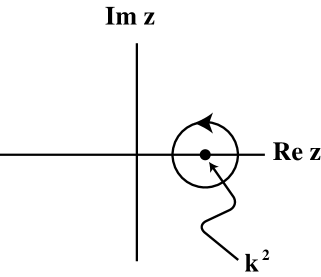
FIG. 1.: The contour utilized in the contour integration identity (E2) for the summand in the correction to the equation of state.

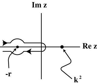
FIG. 2.: The deformation of the contour in Figure 1 that leads to the new expression (E3) for the summand in the correction to the equation of state.

FIG. 3.: The sum $\sum_{\vec{k}}1/(z+k^{2})$, as a function of $zL^{2}$, divided by $L^{2}$. The infinite system limit to the sum has been removed.

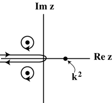
FIG. 4.: The distortion of the contour displayed in Figure 1 that leads to the expression (LABEL:lhs1) for the equation of state

REFERENCES

- [1] M. E. Fisher, S.-k. Ma and B. G. Nickel, Phys. Rev. Lett. 29, 917 (1972).
- [2] M. Suzuki, Prog. Theor. Phys. 49, 1106 (1973).
- [3] M. Aizenman and R. Fernández, Lett. Math. Phys. 16, 39 (1988).
- [4] E. Brezin, J. Zinn-Justin and J. C. Le Guillou, J. Math. Phys. 9, L119 (1976).
- [5] J. Fröhlich and T. Spencer, Commun. Math. Phys. 84, 87 (1982).
- [6] M. Fisher, in Critical Phenomena, Proc. 51st Enrico Fermi Summer School, Varenna, edited by M. S. Green (Academic Press, New York, 1972).
- [7] M. Fisher and M. Barber, Phys. Rev. Lett. 28, 1516 (1972)
- [8] M. Barber, in Phase Transitions and Critical Phenomena, v. 8, edited by C. Domb and J. L. Lebowitz (Academic Press, New York, 1983).
- [9] V. Privman, in Finite Size Scaling and Numerical Simulation of Statistical Systems, edited by V. Privman (World Scientific, Singapore, 1990).
- [10] J. G. Brankov, D. M. Danchev, N. S. Tonchev, The Theory of Critical Phenomena in Finite-Size Systems - Scaling and Quantum Effects, World Scientific, Singapore, 2000.
- [11] X. S. Chen and V. Dohm, Physica A 251, 439 (1998).
- [12] X. S. Chen and V. Dohm, Eur. Phys. J. B 10, 687 (1999).
- [13] X. S. Chen and V. Dohm, Eur. Phys. J. B 7, 183 (1999).
- [14] X. S. Chen and V. Dohm, Physica B 284-288, 45 (2000).
- [15] X. S. Chen and V. Dohm, Eur. Phys. J. B 15, 283 (2000).
- [16] E. Brézin, J. Physique 43, 15 (1982).
- [17] E. Brézin and J. Zinn-Justin, Nuclear Physics B 257, 867 (1985).
- [18] J. Rudnick, H. Guo, and D. Jasnow, J. Stat. Phys. 41, 353 (1985).
- [19] X. S. Chen and V. Dohm, Phys. Rev. E 63, 16113 (2000).
- [20] E. Luijten, K. Binder and H. W. J. Blöte, Eur. Phys. J. B 9, 289 (1999).
- [21] J. M. Kosterlitz, Phys. Rev. Lett. 37, 1577 (1976).
- [22] J. M. Kosterlitz, J. Phys. C 7, 1046 (1974).
- [23] J. Z. Imbrie and C. M. Newman, Commun. Math. Phys. 118, 303 (1988).
- [24] F. Bayong and H. T. Diep, Phys. Rev. B 59, 11919 (1999).
- [25] S. Romano, Phys. Rev. B 62, 1464 (2000).
- [26] E. Luijten, Phys. Rev. E 60, 7558 (1999).
- [27] K. Binder, Z. Phys. B: Cond. Matter 43, 119 (1981).
- [28] H. Chamati and N. S. Tonchev, Phys. Rev. E 63, 26103 (2001).
- [29] E. Luijten, Int. J. Mod. Phys. C 6, 359 (1995).
- [30] P. P. Ewald, Ann Phys. 64, 253 (1921).
- [31] J. G. Brankov and N. S. Tonchev, J. Stat. Phys. 52, 143 (1988).
- [32] J. G. Brankov, J. Stat. Phys. 56, 309 (1989).
- [33] E. R. Korutcheva, N. S. Tonchev, J. Stat. Phys. 62, 553 (1991).
- [34] S. Singh and R. K. Pathria, Phys. Rev. B 40, 9234 (1989).
- [35] J. Brankov and D. Danchev, J. Math. Phys. 32, 9234 (1991).
- [36] M. Abramowitz and I. A. Stegun, Handbook of Mathematical Functions, Dover Publications Inc., New York (1970).
- [37] J. Shapiro and J. Rudnick, J. Stat. Phys. 43, 51 (1986).
- [38] H. Chamati and N. Tonchev, J. Phys. A 33, L167 (2000).