How does the chain extension of poly (acrylic acid) scale in aqueous solution? A combined study with light scattering and computer simulation

Abstract

This work adresses the question of the scaling behaviour of polyelectrolytes in solution for a realistic prototype: We show results of a combined experimental (light scattering) and theoretical (computer simulations) investigation of structural properties of poly (acrylic acid) (PAA). Experimentally, we determined the molecular weight ($M_{W}$) and the hydrodynamic radius ($R_{H}$) by static light scattering for six different PAA samples in aqueous NaCl-containing solution ($0.1-1$ mol/L) of polydispersity $D_{P}$ between $1.5$ and $1.8$. On the computational side, three different variants of a newly developed mesoscopic force field for PAA were employed to determine $R_{H}$ for monodisperse systems of the same $M_{W}$ as in the experiments. The force field effectively incorporates atomistic information and one coarse-grained bead corresponds to one PAA monomer. We find that $R_{H}$ matches with the experimental data for all investigated samples. The effective scaling exponent for $R_{H}$ is found to be around $0.55$, which is well below its asymptotic value for good solvents. Additionally, data for the radius of gyration ($R_{G}$) are presented.

1 Introduction

Poly (acrylic acid) (PAA) is a water-soluble polyelectrolyte (PE). It is important not only in industrial applications, e.g. flocculants or superabsorbers [1]. Because of its relatively simple chemical repeat unit, it is also a prototype PE model for scientific investigations. Surprisingly, there seems to be no (accurate) data on some solution properties of PAA chains. Quantities which characterize the solution behaviour of isolated polymer chains are the radius of gyration $R_{G}$ and the hydrodynamic radius $R_{H}$. It is the main purpose of this letter to provide reliable values for PAA of different chainlengths.

Two approaches are being used. Experimentally, we determine the size of a polymer coil in solution by dynamic ($R_{H}$) or static ($R_{G}$) light scattering. The measurements were performed using narrow fractions of radically polymerized PAA in order to, on the one hand, minimize effects of polydispersity and to, on the other hand, avoid possible problems of PAA aggregation due to hydrophobic initiators used in anionic polymerization [2]. These data are augmented by results from computer simulations. Simulations have the principal advantage that macroscopic observations can be understood in terms of a microscopic model. We will use them here to investigate the scaling of the polymer also at length scales shorter than the overall coil size ($R_{G}$ or $R_{H}$) which is accessible by the light-scattering experiment. This is the second aim of this work.

The experimentally relevant molecular weights are far beyond what can be simulated with an atomistic model. They are, however, accessible with suitably simplified or ”coarse-grained” (CG) models. Care has to be taken that the CG model retains sufficient information about the chemical nature of the polymer. A generic bead-spring model might be good enough for theoretical scaling relations [3, 4, 5], but will not give realistic absolute values for $R_{H}$ of specific polymers like PAA. A number of systematic coarse-graining procedures have been described [6, 7, 8, 9, 10, 11, 12, 13, 14, 15, 16], but none has been tried for specific PEs in solution. We have recently developed an automatic coarse-graining method which works by a two-step process: Firstly, an atomistic simulation of a PAA oligomer in water is performed. Secondly, the CG model is parametrized to reproduce the PAA structure [17]. To validate this method and to try out technical variants on it is the third objective of the letter.

2 Methods

2.1 Experimental

2.1.1 Static and Dynamic Light Scattering

For simultaneous static and dynamic light scattering measurements a commercial instrument (ALV-5000) with a krypton ion laser operating at a wavelength of 647 nm and an Avalanche Diode (EG&G) as detector was used [18]. Static measurements were performed at scattering angles of $30^{\circ}-150^{\circ}$ in $10^{\circ}$ steps in the concentration range of $0.5-5$ g/L. For the high molecular weights the highest concentration was only $3.5$ g/L in order to remain in the dilute regime. Weight average molar masses $M_{W}$ and radii of gyration $R_{G}$ were obtained by Zimm extrapolation using the Rayleigh ratio $RR=1.270~{}{\mathrm{cm}}^{-1}$. The refractive index increments $dn/dc$ are listed in Table 2, as measured at $\lambda=663$ nm using a scanning Michelson interferometer  [19].

Dynamic measurements were performed over an angle range from $60^{\circ}-150^{\circ}$ in $30^{\circ}$ steps. The intensity autocorrelation function of the scattered intensity was converted to the scattered electric field and analyzed using the program CONTIN by S.Provencher [20]. Hydrodynamic radii $R_{H}$ were obtained via the Stokes-Einstein relation, where the apparent diffusion coefficient $D=\Gamma/q^{2}$ was calculated from the inverse relaxation time $\Gamma$ and the absolute value $q$ of the scattering vector.[21] Viscosity corrections due to the NaCl were considered to be small and not taken into account. The hydrodynamic radius $R_{H}$ was measured repeatedly. In Figure 2 the average values and error bars representing one standard deviation are plotted.

2.1.2 Sample Preparation

The PAA samples (Polymer Standard Service) with molar masses of $M_{W}=18000-296600$ g/mol were synthesized by radical polymerization and fractionated with polydispersities $D_{P}=M_{W}/M_{N}$ between 1.5 and 1.8 (with $M_{N}$ being the number average molecular weight). All samples were dissolved in deionized water (Millipore) with $1M$ NaCl. The $pH$ was determined for two samples ($M_{W}=81800$ and $296600$) at two different concentrations ($1$ g/L and $5$ g/L) and found to lie between $6-8$. After further purification, we performed additional measurements by dialysis using a regenerated cellulose membran (MWCO2000). The dialysis process lasted 40 hours and the deionized water (Millipore) was replaced four times. Afterwards, the samples were freeze-dried for 5 hours and finally dried under vaccuum for 60 hours at $T=303$ K, in order to avoid fluctuations of the PAA concentration by adsorbed water. The refractive index increments for the dialyzed and dried samples remained unchanged within the statistical errors. All solutions were filtered through a $0.22$ $\mu$m Millex-GS filter (Millipore) to remove dust particles.

2.2 Computational

2.2.1 The Coarse-grained Force Field for PAA

Coarse-grained potential energy functions for polymers have to incorporate not only energetic, i.e. local aspects of the underlying microscopic model. They also have to account for entropic contributions from the neglected conformational degrees of freedom of the chain. Therefore, we utilized structural information obtained from fully atomistic simulations as target functions to construct our CG force field. In particular, we used the intra- and inter-chain radial distribution functions which, being distributions derived from an ensemble, contain the desired entropic information. This is a so-called inverse problem: find an interparticle potential which reproduces a given radial distribution function (RDF) or set of RDFs. For the fitting procedure, we applied an automatic optimization algorithm (simplex) which was originally implemented for the development of atomistic force fields [22] and tested for liquids.[23] Our force field is based on atomistic simulation data by Biermann et al.[24]. They studied one fully deprotonated, atactic oligomer of 23 monomers with 23 Na⁺ counterions in 3684 water molecules (simple point charge (SPC) model [25]) at ambient conditions. The system represents a diluted ($\approx 2.3$wt$\%$) PAA solution. From this simulation, structural information like the distributions of bond angles or RDFs between monomers were extracted. We mapped this system to the mesoscale by replacing each repeat unit (i.e. each monomer) by one bead, either at the monomers center of mass or at the backbone carbon bearing the carboxyl group. The PAA mesoscale force field includes bonded and non-bonded interactions. To both contribute several terms [26]. They were parametrised by systematically varying the interactions until the structure of the atomistic model was reproduced. This also allowed us to omit all explicit water molecules and counter ions. Their effect on the PAA chain conformation is, however, implicitly present in the model. In effect, a system of roughly $10000$ Atoms could thus be reduced to a system which consists of only $23$ ”superatoms”.

For the sake of gaining experience with CG force fields, we have coarse-grained PAA in three different ways. Potential $I$ is pieced together from various analytic functions. It contains attractive as well as repulsive intermolecular interactions. Coulomb forces were only implicitly taken into account (they were present in the parent atomistic simulation). That is because the Debye length (characterizing the relative importance of the electrostatic energy compared to thermal energy) of the system is close to that of water, so that electrostatic interactions can be treated as being short-ranged. For details, see ref 17. Potential $II$ is similar in construction, but uses another location of the CG bead: While Potential $I$ placed it at the center of mass of a monomer, Potential $II$ employed the backbone carbon parent to the COO^--group [27]. As example for the achieved convergence, the RDF (first neighbours excluded) is shown in Figure 1a. Potential $III$ uses again the center-of-mass of the PAA monomer, but was optimized with a fully numerical instead of a piecewise analytical potential energy function for the non-bonded interactions [27]. It allows us to apply a new self-consistent optimization algorithm which was recently adapted by us. [28] The optimization then yields an almost perfect match of the RDF. Target RDFs (exluding first and second neighbours, as defined in Ref.[17]) and the results of the optimization are shown in Figure 1b. The parameters of force fields $I$ and $II$ are presented in Table 1. The non-bonded part of Potential $III$ exists in numerical form only [27] (not shown here).

2.2.2 Technical Simulation Details

Both Brownian Dynamics (BD) and Monte Carlo (MC) programs were used to carry out the PAA simulations. We simulated at $T=333.15$ K, which corresponds to the temperature of the atomistic simulations. The Langevin equations of motion were integrated by the velocity Verlet algorithm with a time step $\Delta t=0.01\tau$,[29] and a friction constant $\gamma=0.5\tau^{-1}$.[30] Pivot MC calculations were necessary to simulate systems of more than $1000$ monomers as the equilibration is much faster. We carried out $10^{5}$ accepted equilibration moves before a production run of $10^{6}$ accepted moves started.

3 Results and Discussion

The hydrodynamic radii of six different PAA samples with molecular weights in the range from $18100$ to $296600$ g/mol were measured (see Table 2). For four samples, the molar masses $M_{W}$ and the radii of gyration $R_{\mathrm{G}}$ were measured in 1M NaCl solution. (For the samples of lower molecular weight an accurate determination of $R_{G}$ was not possible, so they are reported as specified by the supplier.) Additionally, the ratio $R_{G}/R_{H}$ and the refractive index increment $\partial n/\partial c$ are shown in Table 2. In all PAA solutions, the salt content was so high that the electrostatic interactions were effectively screened. Therefore, $R_{G}$ could be obtained from the static scattering experiment by Zimm extrapolation to zero angle and zero polymer concentration $c_{p}$ like for uncharged polymers. The dynamic measurements in $1$M NaCl solution yielded single-exponential autocorrelation functions, since we performed our measurements in the ”ordinary regime” where $c^{\mathrm{m}}/c_{\mathrm{s}}^{\mathrm{m}}<1$, with $c^{\mathrm{m}}$ and $c_{\mathrm{s}}^{\mathrm{m}}$ being the molar concentration of monomer units and of salt, respectively.[31] No polyelectrolyte slow mode due to a cooperative diffusion behavior was observed. Furthermore, the diffusion coefficients do not show any significant angular dependence.

For two samples with molecular weigths of $M_{W}=119800$ g/mol and $M_{W}=204000$ g/mol, we varied the NaCl concentration between $0.1-1$ mol/L at a fixed polymer concentration of $1$ g/L, as shown in Figure 2a. No dependence of the diffusion coefficient or $R_{H}$ is found within this range. Figure 2b shows a weak decrease of $R_{H}$ with polymer concentration in the range of $0-5$ g/L for two molecular weights $M_{W}$ at fixed NaCl concentration of $1$ M. For further comparisons we use the values extrapolated to zero concentration. Thus the static as well as dynamic light scattering experiments represent measurements of single polylelectrolyte molecules. The hydrodynamic radii are plotted in Figure 3 as a function of molecular mass. We find a scaling exponent of $\nu=0.56\pm 0.02$. This scaling exponent compares well with CG simulation results (below).

In Table 3, the corresponding theoretical data is presented for $13$ different chain lengths (being single chains, the simulated polymers are monodisperse). They include all the experimental ones when converting the mean molar weights $M_{W}$ into the degree of polymerization. We plotted them in Figure 3a, too. Over the whole range of measured samples, the coincidence is excellent. This is especially remarkable if one considers the fact that the simulation model was developed with a PAA chain consisting of only $23$ monomers.

In order to check the transferability of parameters between oligomer chains of different lengths, we executed new atomistic simulations of shorter chains with the same force field as used by Biermann et al. in their work. [24] The PAA was dissolved in $4000$ water molecules (concentration $c_{p}\approx 1$ g/L) and the total simulation time was $6$ ns. The concentration of sodium counterions was determined to be around $0.44$ mol/L for all atomistic simulations, which lies in the middle of the experimentally tested ones. A ”downward” transferability could be obtained for both samples. The CG model developed for a $23$-monomer chain, faithfully reproduces also the $R_{H}$ and $R_{G}$ of the atomistic $8$- and $12$-mers, cf. Table 3a. It is also interesting to investigate the stability of $R_{H}$ for the various simulation models $I$, $II$ and $III$. As shown in Table 3b, the coincidence is good for all chain lengths. This means that our CG mapping is not unique. Structural properties can be determined from any of the above model variants. That might be of use, if one is interested in properties pertaining to the center-of-mass or of the CH-backbone carbon.

In the following, we focus our attention on the original force field $I$. The simulated $R_{H}$ for chains longer than $100$ monomers was fitted by a power law $R_{H}\propto M_{W}^{\nu}$. The resulting scaling exponent $\nu$ was $0.55\pm 0.02$. If we restrict the fit of the experimental data to the simulated chain lengths, we obtain the same exponent. Experiments and simulation yield, hence, very similar results. It can be concluded that the salt concentration (used in experiments) or sodium counterion concentration (in the parent atomistic simulations) effectively screen the charges of the PAA chain. Thus, the Coulomb potential of PAA is really reduced to an effective short-ranged interaction. For small distances, though, the charges stiffen the chain. This behaviour can be understood in the framework of scaling theory. For a Gaussian chain (model of a linear fully-flexible polymer) in a good solvent, self-avoiding walk (SAW) statistics applies. It yields a scaling exponent of $\nu=0.588$ in the limit of infinitely long chains [4]. This scaling factor is universal, i.e. it is valid for every size-characterizing function, e.g. $R_{G}$ or $R_{H}$. The structur factor $S(q)$, however, is an even better function to investigate. That is, because it scales as $S(q)\propto q^{-1/\nu}$, which we can try to fit for any length scale up to the total size of the polymer. So, local deviations from the global behaviour, as measured by the experiment, can be observed. Figure 3b shows the structure factor of the coarse-grained BD simulation of a PAA $460$-mer. Apart from noise in the region $q>10$, three different regimes can be distinguished: On very short distances (nearest neighbours), the slope equals $-1.65=-1/\nu$, i.e. corresponding to a ”local” scaling exponent of $\nu=0.61$. This is remarkably close to, but larger than the value for a SAW ($0.588$). Compared to a Gaussian chain, this is due to the stiffening bond angle potential of the chain (in the CG picture). Next comes the region in which torsions and non-bonded interactions become important. They introduce even more stiffness, resulting in a large exponent of $\nu=0.82$. Finally, the long-range behaviour sets in ($\nu=0.56$), almost yielding the obtained total scaling exponent for $R_{H}$. So we can conclude that PAA globally behaves like a fully-flexible chain without charges. These results are very similar for any other large-enough PAA sample. We note also that the original target RDF of the 23-mer is reproduced by any $23$-monomer sub-strand of the $460$-mer (data not shown). For $R_{G}$, scaling similar to that of $R_{H}$ is, as expected, obtained in the limit of sufficiently long chains ($>100$ monomers). In Figure 3a, this can be seen by examining the ratio $R_{G}/R_{H}$: a plateau region is reached for long chains, with a value of around $1.5$. This is the value predicted for Gaussian chains. A closer look, however, reveals a monotonically increasing ratio (cf. Table 3), exceeding the value of $1.5$. The reason for this behaviour are the corrections to scaling due to the good solvent statistics of the chain, which have been known for a long time [32]. For $R_{H}$, this motivated the empirical indroduction of an effective exponent $\nu_{eff}\approx 0.55$,[33] which exactly equals our findings. A detailed analysis of these corrections, whose asymptotic value is found to be $R_{G}/R_{H}\approx 1.61$, will be presented elsewhere [34].

Table 1: Parameters for our various coarse-grained force fields. For details, see refs 17 and 27.

(a) bond angle parameters
	Peak #	position	standard deviation	peak height
		[o]	[o]	[height of peak 2]
center of mass
force fields $I$,$III$
	1	88.0	6.8	1.72
	2	116.7	7.4	1.00
backbone carbon
force field $II$
	1	127.4	8.5	1.15
	2	156.4	8.9	1.00

(b) non-bonded parameters
	$\sigma_{1}$	$\varepsilon_{1}$	$\sigma_{2}$	$\varepsilon_{2}$	$\sigma_{3}$	$\varepsilon_{3}$	$\sigma_{4}=r_{cut}$	$\varepsilon_{4}$
original force field
(center of mass) $I$
	0.496	11.30	0.559	0.35	0.775	0.49	1.3	0.05
backbone carbon
force field $II$
	0.496	11.30	0.565	1.20	0.802	0.70	1.3	0.05

Table 2: Experimental hydrodynamic radii $R_{H}$ and radii of gyration $R_{G}$ obtained by dynamic and static light scattering experiments for poly (acrylic acid) of different molecular weights $M_{W}$.

$M_{W}$ [g/mol]	$R_{G}$ [nm]	$R_{H}$ [nm]	$R_{G}/R_{H}$	$\partial n/\partial c$
181001 (193-mer)	-	3.7	-	-
369001 (393-mer)	-	5.3	-	-
818002 (870-mer)	12.9	8.9	1.45	0.1360
1198002 (1287-mer)	14.9	10.4	1.44	0.1452
2040002 (2170-mer)	22.7	15.0	1.51	0.1472
2966002 (3155-mer)	23.8	16.6	1.46	0.1310

¹: $M_{W}$ as specified by the supplier
²: $M_{W}$ determined by own static light scattering

Table 3: Radii of gyration $R_{G}$ and hydrodynamic radii $R_{H}$ for different-size poly (acrylic acid) as obtained by Brownian Dynamics (marked ’1’) and Monte-Carlo (marked ’2’) simulations. In the coarse-grained picture, potentials $I$ and $III$ are different versions of center-of-mass mapped force field, whereas potential $II$ is centered at the backbone carbon of the chain.

Chainlength	$R_{G}$ [nm]	$R_{H}$ [nm]	$R_{G}/R_{H}$
(a) Atomistic Model
8-mer	0.55	0.87	0.63
12-mer	0.77	0.91	0.85
23-mer	1.28	1.19	1.08
(b) Coarse-Grained Model
Potential $I$
8-mer1,2	0.57	0.89	0.64
12-mer1	0.78	0.94	0.83
23-mer1,2	1.25	1.18	1.06
46-mer2	2.0	1.6	1.25
92-mer2	3.1	2.3	1.35
193-mer1	4.8	3.4	1.41
393-mer1	6.8	4.8	1.42
460-mer1	7.7	5.3	1.45
460-mer2	7.9	5.5	1.44
852-mer1	10.8	7.4	1.46
855-mer2	11.3	7.7	1.47
1287-mer1	13.5	9.1	1.48
2067-mer2	18.8	12.4	1.52
3155-mer2	24.1	15.7	1.54
Potential $II$
23-mer1	1.22	1.03	1.18
393-mer1	6.9	4.8	1.43
852-mer1	9.4	6.6	1.42
1287-mer1	14.3	9.0	1.59
Potential $III$
23-mer1	1.26	1.18	1.07
460-mer1	8.6	5.9	1.46
852-mer1	12.2	8.3	1.47
1287-mer1	15.5	10.3	1.51

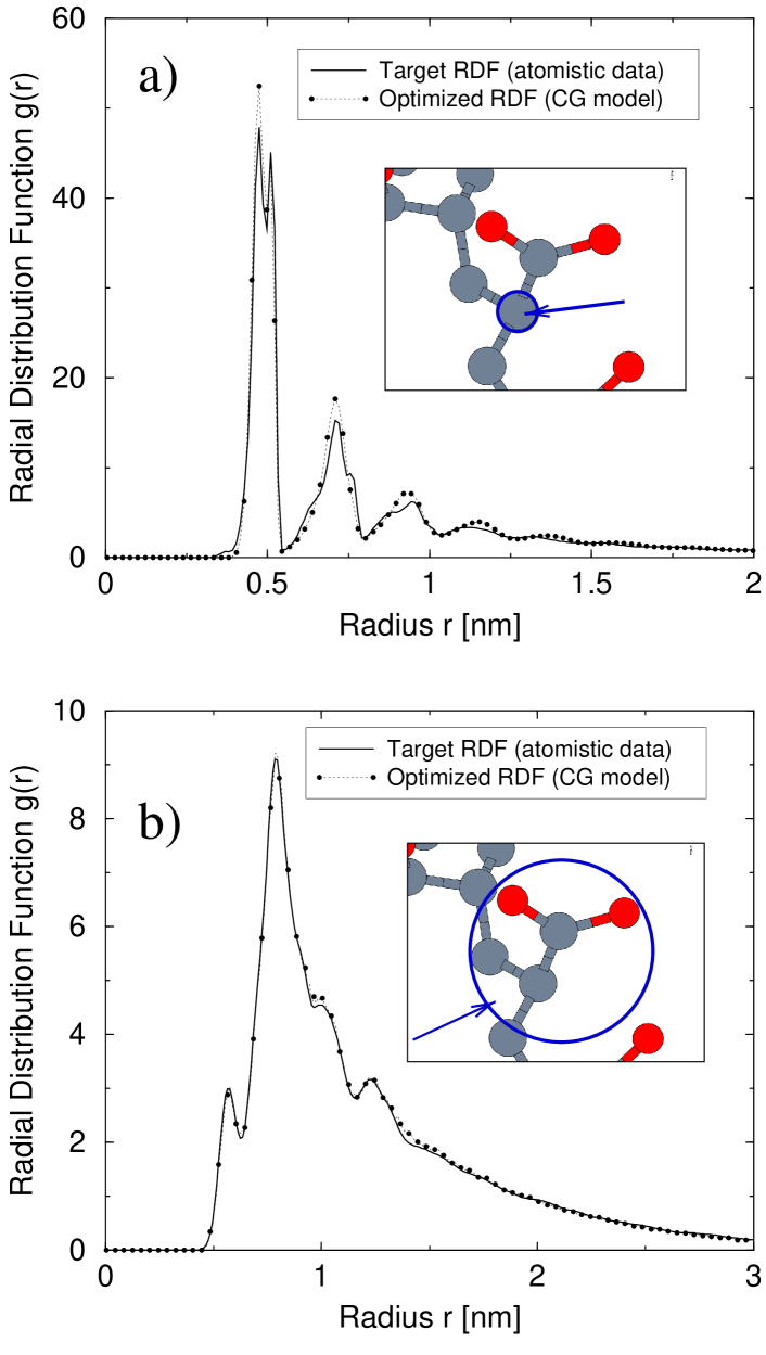
Figure 1:

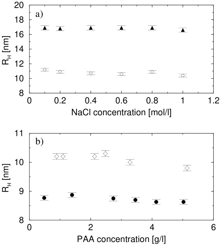
Figure 2:

Figure 3:

References

- [1] des Cloizeaux, J.; Jannink, G.; Polymers in Solution: Their Modelling and Structure; Clarendon Press, Oxford, England; 1990.
- [2] Huber, K.; personal communication; 2000.
- [3] de Gennes, P.-G.; Scaling Concepts in Polymer Physics; Cornell University Press; Ithaca and London; 1979.
- [4] Doi, M.; Edwards, S.; The Theory of Polymer Dynamics; Clarendon; Oxford; 1986.
- [5] Barrat, J.-L.; Joanny, J.-F.; Adv. Chem. Phys. 1996; 94, 1.
- [6] Flory, P.; Statistical Mechanics of Chain Molecules; Carl Hanser Verlag; Munich; 1989.
- [7] Ryckaert, J.-P.; Bellemans, A.; Chem. Phys. Lett. 1975; 30, 123–5.
- [8] Carmesin, I.; Kremer, K.; Macromolecules 1988; 21, 2819–2823.
- [9] Paul, W.; Binder, K.; Kremer, K.; Heermann, D.; Macromolecules 1991; 24, 6332–4.
- [10] Hoogerbrugge, P.; Koelman, J.; Europhys. Lett. 1992; 19, 155.
- [11] Forrest, B.; Suter, U.; J. Chem. Phys. 1995; 102, 7256–66.
- [12] Rapold, R.; Mattice, W.; J. Chem. Soc. Faraday Trans. 1995; 91, 2435–41.
- [13] Zimmer, K.; Linke, A.; Heermann, D.; Batoulis, J.; Burger, T.; Macromol. Theor. Simul. 1996; 5, 1065–74.
- [14] Ahlrichs, P.; Dünweg, B.; Int. J. Mod. Phys. C 1998; 9, 1429.
- [15] Eilhard, J.; Zirkel, A.; Tschöp, W.; Hahn, O.; Kremer, K.; Scharpf, O.; Richter, D.; Buchenau, U.; J. Chem. Phys. 1999; 110, 1819–30.
- [16] Akkermans, R.; Briels, W.; J. Chem. Phys. 2001; 114, 1020–31.
- [17] Reith, D.; Meyer, H.; Müller-Plathe, F.; Macromolecules 2001; 34, in press.
- [18] Vanhee, S.; Rulkens, R.; U.Lehmann; Rosenauer, C.; Schulze, M.; Köhler, W.; Wegner, G.; Macromolecules 1996; 29, 5136.
- [19] Becker, A.; Köhler, W.; Müller, B.; Ber. Bunsen-Ges. Phys. Chem. 1995; 99, 600.
- [20] Provencher, S.; Comput. Phys. Commun. 1982; 27, 229.
- [21] Berne, B.; Pecora, R.; Dynamic Light scattering; John Wiley and Sons, New York; 1976.
- [22] Faller, R.; Schmitz, H.; Biermann, O.; Müller-Plathe, F.; J. Comput. Chem. 1999; 20, 1009–17.
- [23] Meyer, H.; Biermann, O.; Faller, R.; Reith, D.; Müller-Plathe, F.; J. Chem. Phys. 2000; 113, 6264–75.
- [24] Biermann, O.; Hädicke, E.; Koltzenburg, S.; Seufert, M.; Müller-Plathe, F.; Macromolecules 2001; submitted.
- [25] Berendsen, H.; Postma, J.; van Gunsteren, W.; Hermans, J.; in Pullman, B., ed., Intermolecular Forces. D. Reidel Publishing Company; 1981; 1981 pp. 331–42.
- [26] Jensen, F.; Introduction to Computational Chemistry; John Wiley & Sons Ltd., Chichester; 1999.
- [27] Reith, D.; Ph.D. thesis; University of Mainz; 2001; in preparation.
- [28] Pütz, M.; Reith, D.; 2001; in preparation.
- [29] Allen, M.; Tildesley, D.; Computer Simulation of Liquids; Oxford Science; Oxford; 1987.
- [30] Grest, G.; Kremer, K.; Phys. Rev. A 1986; 33, 3628–31.
- [31] Dautzenberg, H.; Jaeger, W.; Kötz, J.; Phillipp, B.; Seidel, C.; Stscherbina, D.; Polyelectrolytes; Hanser Verlag; Munich; 1994.
- [32] Batoulis, J.; Kremer, K.; Macromolecules 1989; 22, 4277–85.
- [33] Adam, M.; Delsanti, M.; J. Physique 1976; 37, 1045–49.
- [34] Dünweg, B.; Reith, D.; 2001; in preparation.