Transport Properties Calculation in the Superconducting State for a Quasi-Twodimensional System

Abstract

We performed a self-consistent calculation of the transport properties of a $d$-wave superconductor. We used for calculations the T-matrix approximation. The coresponding equations were evaluated numerically directly on the real frequecy axis. We studied the $ab$-plane charge dynamics in the coherent limit. For the $c$-axis charge dynamics, we considered both, the coherent and the incoherent limit. We also have calculated the penetration depth in this model.
Keywords: T-matrix approximation, charge dynamics, penetration depth.

]

I Introduction

Although, a large number of experimental and theoretical investigations indicate that two dimensionality of the normal and superconducting state is one of the key factors in high temperature superconductivity [1, 2], it remains to examine whether the cuprates are two-dimensional ($2D$) metals or three-dimensional ($3D$) metals with strong anisotropy. The high temperature superconductors show remarkable deviation from Fermi liquid behavior in the normal state, such as the appearance of the pseudogap phenomena and their related issues. The pseudogap phenomena mean the suppression of the low frequency spectral weight without any long range order. There are enormous studies from both experimental [3] and theoretical point of view [4] in order to explain these phenomena. The direct measurements of electronic spectrum such as $ARPES$ [5] have indicated the similarity between the pseudogap and superconducting gap while using Intrinsic Tunneling Spectroscopy [6], it was found that the pseudogap, is coexisting with the superconducting gap, indicating a different nature of the two phenomena. The crucial test for superconducting origin of the gaps is their magnetic field dependencies. Magnetic field is a strong depairing factor and destroys superconductivity when the field exceeds the upper critical field $H_{c2}$.

The opening of the pseudogap has drastic effect on the physical properties of the high $T_{c}$ cuprates. It is found that associated with the pseudogap the in-plane resistivity deviates from the $T$-linear behavior [7] and the $T$ coefficient of the $c$-axis resistivity changes sign, signaling semiconductor like behavior [8]. A remarkable point of the pseudogap is that it’s structure in momentum space is the same as the superconducting $d_{x^{2}-y^{2}}$ symmetry with continuous evolution through $T_{c}$[9]. This implies that the pseudogap phenomena have close connection to the superconducting fluctuations [10], and strongly suggested that the pseudogap is a precursor of the superconductivity [11]. The main difference between the superconducting gap and the pseudogap is that the gap function is caused by the superconducting order, while the pseudogap is caused by the superconducting fluctuations. The optical conductivity is one of the quantities which most evidently display the anisotropy of the system. Measurements of the $ab$-plane conductivity suggest that the conductance in plane is coherent both in underdoped and overdoped regimes while the $c$-axis conductivity changes in character from a coherent behavior in overdoped regime to an incoherent behavior in the underdoped regime [12]. Theoretical investigations of the $ab$-plane and $c$-axis conductivity both in the normal and superconducting phase can be found in [13].

In this paper we extend the self-consistent T-matrix calculation to the superconducting state. We consider the effects of the superconducting fluctuations on the electronic state which are the origin of the pseudogap. In the superconducting state the T-matrix approximation includes both the amplitude and the phase mode of the superconductor order parameter. We investigate the transport properties which show the pseudogap phenomena. We calculate their behavior in the superconducting state. The normal state behavior was calculated in [14]. This paper is constructed as follows. In section II we give the Hamiltonian and explain the theoretical framework. In section III we present the results for the spectral function $A({\bf k},\omega)$ and the results for the transport properties studied in this paper. In section IV we present the conclusions.

II Theoretical Framework

A Model Hamiltonian

In this section we present the theoretical framework of this paper. We consider a microscopic model, which incorporates both strong electron fluctuation in the $CuO$ planes and a weak interlayer coupling. The hopping between layers is included in the following Hamiltonian:

$$H=\sum_{l}H_{l}-\sum\limits_{{\bf l}}t_{c}\left(i\right)\left(c_{l{\bf,}i,\sigma}^{+}c_{l+1,i,\sigma}+c_{l+1{\bf,}i,\sigma}^{+}c_{l,i,\sigma}\right)$$ (1)

where $t_{c}$ is the hopping amplitude between layers and $c_{l,i,\sigma}(c_{l{\bf,}i,\sigma}^{+})$ is the annihilation (creation) operator for an electron within the planar site $i$, with spin $\sigma$, in layer $l$. Within each layer we consider the following two-dimensional model Hamiltonian which has $d_{x^{2}-y^{2}}$ symmetry superconducting ground state:

$$H_{l} = \sum\limits_{{\bf k,}\sigma}\varepsilon_{{\bf k}}c_{l{\bf,k},\sigma}^{+}c_{l{\bf,k},\sigma}$$ (3)

$$+\sum\limits_{{\bf k,k}^{\prime}{\bf,}\sigma}V_{{\bf k,k}^{\prime}}c_{l{\bf,k},\uparrow}^{+}c_{l{\bf,k+q},\uparrow}c_{l{\bf,k}^{\prime},\downarrow}^{+}c_{l{\bf,k}^{\prime}-{\bf q},\downarrow}$$

where $c_{{}_{{\bf l,k},\sigma}}(c_{{}_{{\bf l,k},\sigma}}^{+})$ is the annihilation (creation) operator for an electron with momentum ${\bf k}$, and spin $\sigma$ in the layer $l$. The electron dispersion relation is given by:

$$\varepsilon_{{\bf k}}=-2t\left(\cos k_{x}+\cos k_{y}\right)-4t^{\prime}\cos k_{x}\cos k_{y}-\mu$$ (4)

where $t$ and $t^{\prime}$ are the nearest and the next-nearest neighbors hopping amplitudes and $\mu$ is the chemical potential. For now on we will consider $t$ equal to unity and $t^{\prime}=-0.5t.$ The pair interaction is written as:

$$V_{{\bf k,k}^{\prime}}=Vf_{{\bf k,k}^{\prime}}$$ (5)

where

$$f_{{\bf k}}=\cos k_{x}-\cos k_{y}$$ (6)

is the $d_{x^{2}-y^{2}}$ wave factor. In equation (5) $V$ is negative. The important character of high $T_{c}$ cuprates is the momentum dependence of the interlayer hopping matrix element $t_{c}({\bf k})$. The transfer matrix $t_{c}({\bf k})$ obtained by the band calculation [15] is expressed as:

$$t_{c}({\bf k})=\left(cosk_{x}-cosk_{y}\right)^{2}$$ (7)

The large magnitude of the resistivity anisotropy in the normal state reflects that the c-axis mean free path is shorter than the interlayer distance, and the carriers are tightly confined to the $CuO$ planes, and also is the evidence of the incoherent charge dynamics in the $c$-axis direction.

B Self-Consistent T-Matrix Approximation

In this paper we focused on the calculation of the Green function directly on the real frequency axis [16] in order to avoid the difficulties of controlling the accuracy of the calculations used in the numerical analytical continuations from the imaginary to the real axis by Padé algorithm [17]. In the previous paper [14] we presented the self-consistent equations set, which must be solved in order to obtain the Green function in the normal state. In this section we will present the equations only for the superconducting state. In the superconducting state, the self-consistent T-matrix approximation is a conserving approximation in the sense of Baym and Kadanoff [18].

For a continuum model with local interactions, the corresponding equations have been derived by Haussmann [19] and the analogous equations for the Hubbard model by Pedersen et. al. [20]. The equations were solved in [21] and the thermodynamics of a superconductor was also studied. A similar model was also studied in [22].

Here we extend the self-consistent T-matrix calculation to the superconducting state. We carry out a self-consistent calculation for the spectral functions:

$$A({\bf k},\omega)=-\frac{1}{\pi}ImG({\bf k},\omega)$$ (8)

and:

$$B({\bf k},\omega)=-\frac{1}{\pi}ImF({\bf k},\omega)$$ (9)

where the Green function $G({\bf k},\omega)$ is given by:

$$G({\bf k},\omega)=\frac{\omega+\varepsilon_{{\bf k}}+\Sigma(-{\bf k},-\omega)}{\left(\omega-\varepsilon_{{\bf k}}-\Sigma({\bf k},\omega)\right)\left(\omega+\varepsilon_{{\bf k}}+\Sigma(-{\bf k},-\omega)\right)-\Delta_{{\bf k}}^{2}}$$ (10)

and the anomalous Green function $F({\bf k},\omega)$ is given by:

$$F\left({\bf k},\omega\right)=\frac{\Delta_{{\bf k}}}{\left(\omega-\varepsilon_{{\bf k}}-\Sigma({\bf k},\omega)\right)\left(\omega+\varepsilon_{{\bf k}}+\Sigma(-{\bf k},-\omega)\right)-\Delta_{{\bf k}}^{2}}$$ (11)

where $\Sigma({\bf k},\omega)$ is the retarded self-energy and $\Delta_{{\bf k}}$ is the order parameter in the superconducting state. We choose for the gap function $\Delta_{{\bf k}}$ a $d_{x^{2}-y^{2}}$-symmetry form $\Delta_{{\bf k}}=$ $\Delta f_{{\bf k}}$. The imaginary part of the self-energy can be expressed as:

$$Im\Sigma({\bf k},\omega) = f_{{\bf k}}^{2}\sum_{{\bf k}^{\prime}}\int d\omega^{\prime}\left[f(\omega^{\prime})+n(\omega+\omega^{\prime})\right]\times$$ (13)

$$A({\bf k}^{\prime},\omega^{\prime})ImT_{11}({\bf k+k}^{\prime},\omega+\omega^{\prime})$$

where $f(\omega)$ and $n(\omega)$ are the Fermi-Dirac and Bose-Einstein distributions. The real part of the retarded self-energy can be calculated using the Kramers-Krönig relation:

$$Re\Sigma({\bf k},\omega)=p.v.\int\frac{d\omega^{\prime}}{\pi}\frac{Im\Sigma({\bf k}^{\prime},\omega^{\prime})}{\omega-\omega^{\prime}}$$ (14)

where $p.v.$ represent the principal value of the integral. We have to mention that only the diagonal part of the T-matrix is taken into account when we calculated the self-energy. Ignoring the off-diagonal part of the T-matrix means that the anomalous self-energy is not considered. The T-matrix is given by the following relation:

$$T({\bf q},\omega)=V\left[1+V\Pi({\bf q},\omega)\right]^{-1}$$ (15)

where $\Pi({\bf q},\omega)$ is a $2\times 2$ matrix given by:

$$\Pi({\bf q},\omega)=\left(\begin{tabular}[]{ll}$K({\bf q},\omega)$&$L({\bf q},\omega)$\\ $L^{*}({\bf q},\omega)$&$K(-{\bf q},-\omega)$\end{tabular}\right)$$ (16)

The imaginary part of $K({\bf q},\omega)$ and $L({\bf q},\omega)$ can be calculated as follows:

$$ImK({\bf q},\omega) = \pi\sum_{{\bf k}}\int d\omega^{\prime}f_{{\bf k}}^{2}tgh\frac{\omega^{\prime}}{2T}\times$$ (18)

$$A({\bf k},\omega^{\prime})A({\bf q-k},\omega-\omega^{\prime})$$

$$ImL({\bf q},\omega) = \pi\sum_{{\bf k}}\int d\omega^{\prime}f_{{\bf k}}^{2}tgh\frac{\omega^{\prime}}{2T}\times$$ (20)

$$B({\bf k},\omega^{\prime})B({\bf q-k},\omega-\omega^{\prime})$$

The real part of the $K({\bf q},\omega)$ and $L({\bf q},\omega)$ are also calculated using Kramers-Krönig relation. The chemical potential is determined by fixing the carriers density $n$ through the relation:

$$n=2\sum_{{\bf k}}\int d\omega A({\bf k},\omega)f(\omega)$$ (21)

We will consider in the following, the hole doping $\delta=1-n.$ We also have the sum rule which must be satisfied:

$$1=\sum_{{\bf k}}\int d\omega A({\bf k},\omega)$$ (22)

The gap $\Delta$ can be calculated self-consistently using the gap equation which in our notations can be written as:

$$\Delta=V\sum_{{\bf k}}\int d\omega f_{{\bf k}}^{2}B({\bf k},\omega)f(\omega)$$ (23)

Equations (21)-(23) must be satisfied at each step in the self-consistent calculation in order to obtain the new chemical potential and the gap function. We have to mention at this point that we did not take into account the anomalous self-energy at this level of calculations. The gap function can be calculated from the equation: $1+VK({\bf 0},0)-VL({\bf 0},0)=0$, which is equivalent to the gap equation and is realized in the superconducting state. We determined the gap $\Delta_{K}$ using both methods and found similar behavior as function of $T$.

For this calculation we used a Brillouin zone divided into $32\times 32$ lattice and the frequency integration was done over $1024$ points. All the correlations and the convolutions appearing in Eqs. (13)-(23) were done using the $FFT$ algorithm. Performing the self-consistent calculation we obtain the spectral functions $A({\bf k},\omega)$ and $B({\bf k},\omega)$. Using this spectral functions we can calculate different physical characteristics of cuprates. We can also calculate the density of state:

$$N(\omega)=\sum_{{\bf k}}A({\bf k},\omega)$$ (24)

The $ab$-plane conductivity can be calculated using the following relation [13]:

$$\sigma_{ab}(\nu) = -\frac{e^{2}}{d}\frac{1}{\omega}\sum_{{\bf k}}\left[\left(\frac{\partial\varepsilon_{{\bf k}}}{\partial k_{x}}\right)^{2}+\left(\frac{\partial\varepsilon_{{\bf k}}}{\partial k_{y}}\right)^{2}\right]\times$$ (27)

$$\int\frac{d\omega^{\prime}}{\pi}\left[f(\omega^{\prime}+\omega)-f(\omega^{\prime})\right]\times$$

$$\left[A({\bf k},\omega^{\prime})A({\bf k},\omega+\omega^{\prime})+B({\bf k},\omega^{\prime})B({\bf k},\omega+\omega^{\prime})\right]$$

The equation (27) for the $ab$-plane conductivity neglects the vertex corrections and is coherent in character. For the calculation of $c$-axis conductivity we consider both the coherent and incoherent limits. The coherent $c$-axis conductivity is given by the relation:

$$\sigma_{c}(\omega) = -de^{2}\frac{1}{\omega}\sum_{{\bf k}}t_{c}^{2}({\bf k})\int\frac{d\omega^{\prime}}{\pi}\left[f(\omega^{\prime}+\omega)-f(\omega^{\prime})\right]\times$$ (29)

$$\left[A({\bf k},\omega^{\prime})A({\bf k},\omega+\omega^{\prime})+B({\bf k},\omega^{\prime})B({\bf k},\omega+\omega^{\prime})\right]$$

In equations (27)-(29) $d$ represents the interlayer distance. The contribution from the incoherent process has been discussed by different authors [23]. The contribution from the tunneling process can be written as:

$$\sigma_{inc}(\omega) = -de^{2}\frac{1}{\omega}\sum_{{\bf k,k}^{\prime}}\int\frac{d\omega^{\prime}}{\pi}\left[f(\omega^{\prime}+\omega)-f(\omega^{\prime})\right]\times$$ (31)

$$A({\bf k},\omega^{\prime})A({\bf k}^{\prime},\omega+\omega^{\prime})$$

We calculate also, the London penetration depth. This quantity is proportional with the superfluid density. The in-plane penetration depth is given by:

$$\frac{1}{\lambda_{ab}^{2}}=2\frac{e^{2}}{d}\sum_{{\bf k}}\int d\omega\left[\left(\frac{\partial\varepsilon_{{\bf k}}}{\partial k_{x}}\right)^{2}+\left(\frac{\partial\varepsilon_{{\bf k}}}{\partial k_{y}}\right)^{2}\right]\left|F({\bf k},\omega)\right|^{2}f\left(\omega\right)$$ (32)

and the $c$-axis penetration depth is:

$$\frac{1}{\lambda_{c}^{2}}=8de^{2}\frac{1}{\omega}\sum_{{\bf k}}\int d\omega t_{c}^{2}({\bf k})\left|F({\bf k},\omega)\right|^{2}f\left(\omega\right)$$ (33)

In the next section we present the results obtained for the transport properties calculated in this paper and compare the results with other theoretical works and with experimental data.

III Results

In this section we present the results obtained for the self-consistent T-matrix approximation set of equations, introduced in the previous section. Through out of our calculation we chose for the coupling constant $V=-5.5t.$ To study the superconducting state, we first calculated superconducting transition temperature $T_{c}$. The superconducting transition temperature was determined as the highest temperature where the set of equations (8)-(23) has a non zero solution for the gap function. Near the critical temperature the algoritm becomes unstable because of the rapid growth of order parameter which was found also in the $FLEX$ calculations in [24], caused by the depairing effect due to low frequency spin fluctuations. In our case we consider the effect of the superconducting fluctuations. The effect is included in the retarded self-energy, which is determined self-consistently. Using T-matrix approximation we include both the amplitude and phase mode of the superconducting fluctuations in the self-energy [25]. The self-energy corrections are reduced in the superconducting state because the fluctuations are reduced. The T-matrix approximation gives a unified description for the normal state in the pseudogap region of the underdoped cuprates and the superconducting state [14]. The approximation is not accurate near the critical temperature $T_{c}$ because of the strong suppression of the depairing effect due to the pseudogap, followed by rapid growth of superconducting gap below $T_{c}.$ The order parameter grows more rapidly than in the $BCS$ model. We chose $\delta=0.15$ as the hole concentration. We found the $BCS$ critical temperature $T_{BCS}=0.37t$ and in the case of the self-consistent calculations $T_{C}=0.22t$. In $Fig.1$ we present the order parameter $\Delta$ as function of temperature.

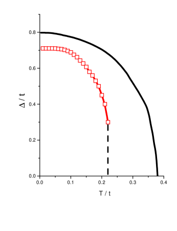
Fig. 1.: Temperature dependence of the order parameter $\Delta$. The solid line represents the $BCS$ gap function while the symbols line represent the self-consistent gap function.

After performing the self-consistent calculation we can calculate the transport properties of the system. The penetration depth can be calculated along the $ab$-plane and c-axis directions, using Eqs. (32) and (33). In $Fig.2$ and $Fig.3$, we present the temperature dependence of the penetration depth as function of temperature

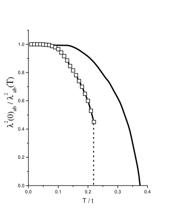
Fig. 2.: Temperature dependence of the in-plane penetration depth in the $BCS$ model (solid line) and the self-consistent calculation (symbols line)

We found a similar behavior as in the case of $BCS$ model. Due to the rapid increase of the order parameter blow $T_{C}$ we found a rapid decrease of the penetration depth with decreasing temperature in both $ab$-plane and $c$-axis directions. Recently, the penetration depth was measured as function of temperature by different authors for $YBCO$ and $Bi-2212$ using different techniques [26]. The magnetic field penetration depth $\lambda$ of superconductors is related to the superconducting carrier density $n_{s}$ divided by the effective mass $m^{*}$ as $1/\lambda^{2}\propto n_{s}/m^{*}$. In a recent paper Uemura [27] explained the experimental data found in [28] assuming a microscopic phase separation between superfluid and non-superconducting fermionic carriers, similar to the superfluid $He$ films.

Fig. 3.: Temperature dependence of the $c$-axis penetration depth in the $BCS$ model (solid line) and the self-consistent calculation (symbols line)

Recently, it was reported that, the photoemission spectra near the Brillouin zone boundary, exhibit unexpected sensitivity to the superfluid density [29], supporting the universality as function of doping and temperature of the properties of the cuprates. We did not consider the vertex corrections for the calculation of $F({\bf k},\omega)$. Desired improvements of the present approach include the consideration of the vertex corrections neglected in the present approach.

We also analyze the $ab$-plane and $c$-axis optical conductivity in the superconducting state using the same approximation. For the calculation of $\sigma_{ab}$ we consider a coherent nature of the interlayer coupling. For the $c$-axis conductivity we consider the coherent and the incoherent coupling. Coherent coupling originates from an overlap of electronic wave functions between planes, and in-plane momentum is conserved in interlayer hopping. By contrast, for impurity mediated incoherent coupling, the in-plane momentum is not conserved.

The influence of the nature of the interlayer coupling on $c$-axis conductivity was studied by different authors [13, 30]. The $ab$-plane conductivity is mainly due to the quasiparticles near the ’cold points’, although the $c$-axis conductivity is due to the quasiparticles near the ’hot points’. Since the superconducting $d_{x^{2}-y^{2}}$ gap and the pseudogap in the underdoped region above $T_{c}$ are large at ’hot points’, the $c$-axis conductivity reflects the pseudogap more clearly then the $ab$-plane conductivity.

In $Fig.4$ we present the calculated $\sigma_{ab}$, based on Eq. (27). The behavior in the superconducting state is similar with the behavior in the normal state.

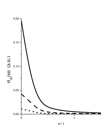
Fig. 4.: Frequency dependence of the $ab$-plane conductivity for different temperatures. The solid line corresponds to $T=0.19t$, the dashed line to $T=0.1t$ and the dotted line to $T=0.07t$. The critical temperature is $T_{C}=0.22t$.

The in-plane spectrum is dominated by a Drude peak at $\omega=0$. The intensity of the peak, increases with increasing temperature. Below $T_{c}$ there is no signature of superconducting gap seen in $YBa_{2}Cu_{3}O_{7-\delta}$ [12]. Careful study of optical conductivity by different methods shows that the width of the Drude peak diminished by several orders of magnitude by decreasing the temperature, just below $T_{c}$ [31]. In cuprates, in contrast with $BCS$ theory, the excitations are electronic, and as the gap develops in this excitations, the decrease in the scattering take place. The optical properties of the cuprates, are those of a clean limit of a $BCS$ superconductor. For the calculations of the $c$-axis conductivity we consider both the coherent and the incoherent nature of the interlayer coupling.

In $Fig.5$ we present the results for the $c$-axis optical conductivity in the case of the coherent nature of the interlayer coupling. The approximation assumes the independent electron propagation in each layer and is justified for $t_{c}\ll t$. In this case, the $\sigma_{c}$ spectrum is dominated by a Drude peak at $\omega=0$. This features are characteristics of the $d$-wave symmetry, and due to the contribution from the gap node.

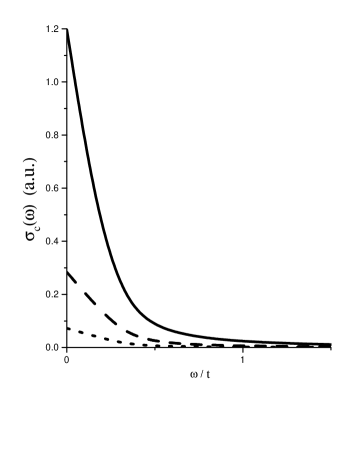
Fig. 5.: Frequency dependence of the coherent $c$-axis conductivity for different temperatures. The solid line corresponds to $T=0.19t$, the dashed line to $T=0.1t$ and the dotted line to $T=0.07t$. The critical temperature is $T_{C}=0.22t$.

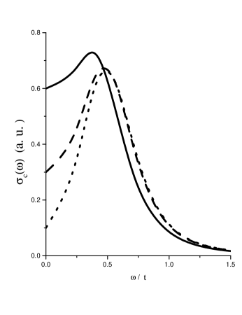
Fig. 6.: Frequency dependence of the incoherent $c$-axis conductivity for different temperatures. The solid line corresponds to $T=0.19t$, the dashed line to $T=0.1t$ and the dotted line to $T=0.07t$. The critical temperature is $T_{C}=0.22t$.

In $Fig.6$, the results for the $c$-axis conductivity are presented in the limit of the incoherent nature of the interlayer coupling. In this case the electronic contribution to $\sigma_{c}\left(\omega\right)$ does not form a Drude peak at $\omega=0$ [32]. In the superconducting state, the $c$-axis optical conductivity is suppressed furthermore with decreasing temperature and shows the gap structure at low temperatures. We consider both limit, because measurements of $c$-axis conductivity suggest that conductance in $c$-direction is coherent in the overdoped regime [33], and incoherent in the underdoped regime [12]. The coherent $\sigma_{c}$ was calculated using Eq. (29) and the incoherent $\sigma_{c}$ using Eq. (31).

The results presented in $Fig.6$ are in agreement with the experimental results obtained for the underdoped $YBa_{2}Cu_{3}O_{7-\delta}$. Here we calculate the conductivity by neglected the vertex corrections. The vertex correction is not important, except for the Umklapp scattering in the case of electron correlation [34].

IV Conclusions

Solving the self-consistent T-matrix equations for the model presented in the section 2 we have computed the transport properties of the system in the superconducting state. Calculations were performed for the superconducting order parameter of $d_{x^{2}-y^{2}}$ symmetry. The effect of the superconducting fluctuations is included in the self-energy corrections. It is clear that the T-Matrix approximation breaks down in the limit $T\rightarrow T_{C}$ since the propagator is dramatically renormalized at the Fermi level. Our scenario is based on resonance scattering [11]. The gap function was found to develop more rapidly than in the $BCS$ model. We calculated the London penetration depth and the $c$-axis and $ab$-plane conductivity and compared the results with the experimental data. The study of experimental dependence of the penetration depth is an important problem [27, 28].

Desired improvements of the present approach include the considerations of the vertex corrections neglected in this approximation. The vertex corrections have a significant effect in the calculation of Hall resistivity [35] and magnetoresistance [36] in high-$T_{c}$ superconductors. Although, the effect was suggested to be insignificant to superconductivity [37], a self-consistent calculation included vertex corrections is desired.

REFERENCES

- [1] P. W. Anderson et al. Phys. Rev. Lett 60, 132, (1988)
- [2] P. B. Littlewood et al. Phys. Rev. B 45, 12636, (1992)
- [3] M. Imada, A. Fujimori and Y. Tokura Rev. Mod. Phys. 70, 1039, (1998)
- [4] T. Dahm, D. Manske and L. Tewordt Phys. Rev. B55, 15274, (1997) V. J. Emery, S. A. Kivelson and O. Zachar Phys. Rev. B56, 6120, (1997) H. Fukuyama, H. Kohno, B. Normand and T. Tanamoto J. Low. Temp. Phys. 99, 429, (1995) V. J. Emery, S. A. Kivelson Nature, 374, 434, (1995) J. Schmalian, D. Pines, and B. Stoikovic Phys. Rev. Lett. 80, 3839, (1988) A. V. Chubukov cond-mat/9709221
- [5] H. Ding et al. Nature 382, 51, (1996) M. R. Norman et al. Nature 392, 157, (1998)
- [6] V. M. Krasnov et al. Phys. Rev. Lett. 84, 5860, (2000) V.M.Krasnov et.al. cond-mat/0002094
- [7] T. Ito, K. Takenaka, and S. Uchida Phys. Rev. Lett. 70, 3995, (1995)
- [8] K. Takenaka et al. Phys. Rev. B 50, 6534, (1994)
- [9] G. V. M. Wiliams, J. L. Tallon and J. W. Loram Phys. Rev. B58, 15053, (1998)
- [10] M. Oda et al. Physica C 281, 135, (1997)
- [11] M. Randeria cond-mat/ 9710223 J. Maly, B. Janko and K. Levin Physica C 321, 13, (1999) also cond-mat/9805018
- [12] C. C. Homes, T. Timusk, R. Liang, D. A. Bonn and W. N. Hardy Physica C 254, 265, (1995) S. Uchida Physica C 282-287, 12, (1997) T. Timusk Physica C 317-318, 18, (1999) A. V. Puchkov, D. N. Basov and T. Timusk J. Phys. Condens. Matter 8, 10049 (1996) H. L. Liu et.al. J. Phys. Condens. Matter 11, 239 (1999)
- [13] E. Jekelmann, F. Gebhard and F.H.L. Essler cond-mat/ 9911281 A. Ramsak, I. Sega and P. Prelovsek cond-mat/ 9906333 P. Prelovsek, A. Ramsak and I. Sega, Phys. Rev. Lett. 81, 3745 (1998) P.W. Anderson The Theory of Superconductivity in High- Cuprates Princeton University Press (1997) A. J. Leggett Phys. Rev. Lett. 83, 392, (1999) Y. Yanase and K. Yamada J. Phys. Soc. Jpn. 68, 548, (1999)
- [14] C. P. Moca and E. Macocian (accepted for publication in Physica C), also cond-mat/0011054
- [15] O. K. Andersen et al. J. Phys. Chem. Solids 56, 1573, (1995) S. Chrakavarty et al. Science 261, 337, (1993)
- [16] B. Kyung et al. Phys. Rev. Lett. 80, 3109, (1998)
- [17] H. Vilberg and J. Serene J. Low Temp. Phys. 29, 179, (1997)
- [18] G. Baym and L. P. Kadanoff Phys. Rev. 124, 287, (1961)
- [19] R. Haussmann Z. Phys. B. 91, 291, (1993)
- [20] M. H. Pedersen, J.J. Rodriguez-Nunez, H. Beck, T. Schneider and S. Schafroth Z. Phys. B 103, 21, (1997)
- [21] M. Keller, W. Metzner and U. Schoollwöck Phys. Rev. B60, 3499, (1999)
- [22] S. Schafroth, J.J. Rodriguez-Nunez, H. Beck, J. Phys. Cond. Matter 91, 111, (1997)
- [23] P. J. Hirschfield, S. M. Quinlan and D. J. Scalapino Phys. Rev. B55, 12742, (1997) N. F. Mott and E. A. Davis Electronic processes in non- crystalline materials, Clarendon Press, (1979)
- [24] T. Takimoto and T. Moriya J. Phys. Soc. Jpn. 67, 3570, (1998) also cond-mat/9806009
- [25] Y. Yanase, T. Joju and K. Yamada cond-mat/0010281
- [26] T. Jacobs, S. Sridhar, Q. Li, G. D. Gu, N. Koshizuga Phys. Rev. Lett. 75, 4516, (1995) D. A. Bonn et al. Phys. Rev. B. 50, 4051, (1994) J. E. Sonier et al. Phys. Rev. Lett 83, 4156, (1999)
- [27] Y. J. Uemura cond-mat/0012016
- [28] Y. J. Uemura et al. Phys. Rev. Lett. 62, 2317, (1989) Y. J. Uemura et.al. Phys. Rev. Lett. 66, 2665 (1991) Y. J. Uemura et.al. Nature 364, 605 (1993) J. Nesot et al. Phys. Rev. Lett. 83, 840, (1999)
- [29] D. L. Feng et al. Science 280, 277, (2000)
- [30] W. Kim and J. P. Carbotte cond-mat/0010314
- [31] D. A. Bonn, P. Dosanjh, R. Liang and W. N. Hardy Phys. Rev. Lett. 68, 2390, (1992) D. B. Romero et al. Phys. Rev. Lett. 68, 1590, (1992) M. C. Nuss et al. Phys. Rev. Lett. 66, 3305, (1991)
- [32] K. Tamasaku et al. Phys. Rev. Lett. 72, 3088, (1994)
- [33] C. Bernhard et al. Phys. Rev. Lett. 80, 1762, (1998)
- [34] K. Yamada and K Yoshida Prog. Theor. Phys. 76, 621, (1986)
- [35] H. Kontani, K. Kanki and K. Ueda Phys. Rev. B. 59, 14723, (1999) H. Kontani and H. Kino cond-mat/0011324 K. Kanki and H. Kontani J. Phys. Soc. Jpn. 68, 1614 (1999)
- [36] H. Kontani cond-mat/0011327 H. Kontani cond-mat/0011328
- [37] P. Monthoux Phys. Rev. B. 55, 15261, (1997)