Oscillations of Bose-Einstein condensates with vortex lattices:
Finite temperatures

Abstract

We derive the finite temperature oscillation modes of a harmonically confined Bose-Einstein condensed gas undergoing rigid body rotation supported by a vortex lattice in the condensate. The hydrodynamic modes separate into two classes corresponding to center-of-mass and relative oscillations of the thermal cloud and the condensate. These classes are independent of each other in the case where the thermal cloud is inviscid for all modes studied, except the radial pulsations which couple them because the pressure perturbations of the condensate and the thermal cloud are governed by different adiabatic indices. If the thermal cloud is viscous, the two classes of oscillations are coupled, i.e., each type of motion involves simultaneously mass and entropy currents. The relative oscillations are damped by the mutual friction between the condensate and the thermal cloud mediated by the vortex lattice. The damping is large for the values of the drag-to-lift ratio of the order of unity and becomes increasingly ineffective in either limit of small or large friction. An experimental measurement of a subset of these oscillation modes and their damping can provide information on the values of the phenomenological mutual friction coefficients and the quasiparticle-vortex scattering processes in dilute atomic Bose gases.

I Introduction

Recent experiments on rotating trapped Bose-Einstein condensates have created vortex lattices with large number of vortices either by stirring a condensate with a rotating anisotropic perturbation PARIS1 ; MIT1 ; MIT2 ; OXFORD or by evaporatively cooling a spinning normal gas JILA1 . Being reminiscent of the classical rotating bucket experiments, carried out on superfluid phases of helium, the experiments on rotating Bose-Einstein condensates open a variety of new ways of manipulating a rotating condensate and deducing information on its physical properties PARIS1 ; MIT1 ; MIT2 ; OXFORD ; JILA1 . The aspect ratios of the condensates measured by a non destructive imaging and the deduced number of vortices are consistent with a rigid body rotation of the condensates. The experiments carried out at finite temperatures MIT1 ; JILA1 achieve a rigid body rotation of the thermal cloud at a frequency close to that of the condensate (for example, in the MIT experiment MIT1 the ratio of spin frequencies of the thermal cloud to that of the condensate is close to 2/3). These systems contain typically $10^{5}$-$10^{6}$ particles and the fluid hydrodynamics is well suited for the studies of their confined state. The range of rotation rates covered by the experiments extends up to the centrifugal limit: by combining the evaporative cooling and optical spin-up techniques rotation rates larger than 99$\%$ of the centrifugal limit were achieved for a harmonic confinement JILA2 ; rotation rates beyond the centrifugal limit were reached by a sequential laser stirring of a condensate confined in a combination of a quadratic and quartic potentials PARIS2 .

In this paper we address the oscillations and stability of a harmonically confined, rotating Bose-Einstein condesate at finite temperatures in the hydrodynamic regime. The angular momentum of the superfluid is carried by singly quantized vortices which form a triangular Abrikosov lattice. We work in the limit of coarse-grained hydrodynamics, where the physical quantities are averages over large number of vortices. In this limit the structure of individual vortices is unresolved and the superfluid simply mimics a rigid body rotation at the frequency $\Omega=\kappa n_{V}/2$, where $\kappa=2\pi\hbar/m$ is the quantum of circulation, $n_{V}$ is the vortex density in the plane orthogonal to the spin vector, $m$ is the boson mass. The hydrodynamic approximation to the microscopic dynamics of the Bose-Einstein condesate is justified in the regime of strong interparticle interactions and large number of particle in the system (the strong-coupling regime requires $Na/d\gg 1$ where $N$ is the net number of particles in the condensate, $a$ is the scattering length, and $d=\sqrt{\hbar/m\omega_{0}}$ is the oscillator length defined in terms of oscillator frequency $\omega_{0}$). The Thomas-Fermi approximation is valid for systems with large number of particles and insures that quantum corrections (such as the ‘quantum pressure’ term) to the hydrodynamic equations can be neglected. In addition, for large enough systems the space-local values of the thermodynamic quantities such as the pressure and chemical potential are well defined. For such systems the coherence length of the condensate $\xi=1/\sqrt{8\pi na}$, where $n$ is the number density of the condensate particles, becomes much smaller than the intervortex distance and the vortex cores can be treated as singularities in the hydrodynamic equations.

Compared to the zero-temperature case the number of degrees of freedom of a Bose-Einstein condesate is doubled at finite temperatures and so is the number of oscillations modes. The modes can be classified into two subsets, which correspond to the center of mass and relative oscillations of the condensate and the thermal cloud. The first set, which corresponds to density oscillations of the combined fluid (first sound), is identical to the modes of a rotating, zero-temperature condensate in the limit of inviscid normal-fluid and for those modes which do not involve pressure perturbations. These modes were derived within the tensor virial method CHANDRA in a preceding paper  Paper1 (hereafter Paper I). In the special case of an axial-symmetric trap, the lowest-order non-trivial modes (classified by corresponding terms of the expansion of perturbations in spherical harmonics labeled by indices $l,m$) are those with $l=2$ and $-2\leq m\leq 2$. Simple analytical results are available in the case of an axisymmetric trap and we list them below for later references. An analysis of the hydrodynamic modes in Ref. STRINGARI of the even $m$ modes belonging to $l=2$ harmonics is in agreement with the results quoted below. A generalization to odd $m$ and arbitrary $l\geq 2$ harmonics of the surface modes of a rotating condensate is given in Ref. CHEVY . The frequencies of the toroidal modes are given by [Paper I, Eq. (34); our nomenclature follows Ref. CHANDRA ]

$$\sigma_{1,2}(l=2,|m|=2)=\Omega\pm\sqrt{2\omega_{\perp}^{2}-\Omega^{2}},$$ (1)

where $\Omega$ is spin frequency of the condensate, $\omega_{\perp}$ is the component of the trapping frequency orthogonal to the spin vector; two complementary modes follow from the substitution $\Omega\to-\Omega$. The frequencies of the pulsation, or breathing, modes are given by [Paper I, Eq. (45)]

$$\sigma_{1,2}^{2}(l=2,|m|=0) = \frac{3}{2}\omega_{z}^{2}+2\omega_{\perp}^{2}$$ (2)

$$\pm\sqrt{9\omega_{z}^{4}-16(\omega_{z}^{2}\omega_{\perp}^{2}-\omega_{\perp}^{4})-8\omega_{z}^{2}\Omega^{2}},$$

where $\omega_{z}$ is the component of the trapping frequency parallel to the spin vector. Finally, the frequencies of the transverse-shear modes $(l=2,|m|=1)$ are determined by the characteristic equation [Paper I, Eq. (22)]

$$\sigma^{3}-2\Omega\sigma^{2}-(\omega_{\perp}^{2}+\omega_{z}^{2}-\Omega^{2})\sigma+2\Omega\omega_{z}^{2}=0.$$ (3)

There are three distinct modes that solve Eq. (3)

$$\sigma_{1} = \frac{2\Omega}{3}+(s_{+}+s_{-}),$$

$$\sigma_{2,3} = \frac{2\Omega}{3}-\frac{1}{2}(s_{+}+s_{-})\pm\frac{i\sqrt{3}}{2}(s_{+}-s_{-}),$$ (4)

and three complementary modes follow from the substitution $\Omega\to-\Omega$ [see Paper I, Eq. (23) and (24)]. The coefficients in Eqs. (I) are defined as FOOTNOTE

$$s_{\pm}^{3} = \frac{\Omega}{3}\left(\omega_{\perp}^{2}-2\omega_{z}^{2}-\frac{\Omega^{2}}{9}\right)\mp\frac{1}{9}\Bigl{[}\left(\omega_{\perp}^{2}+\omega_{z}^{2}+\frac{\Omega^{2}}{3}\right)^{3}$$ (5)

$$-\Omega^{2}\left(\omega_{\perp}^{2}-2\omega_{z}^{2}-\frac{\Omega^{2}}{9}\right)^{2}\Bigr{]}^{1/2}.$$

As we shall see below, Eqs. (1) and (3)-(5) remain valid at finite temperatures when the viscosity of the thermal cloud is negligible; Eq. (2) will be modified since the pulsations of the condensate and the thermal cloud couple due to the difference in the underlying equations of state of these components. In the two fluid setting these equations correspond to the first class of the center of mass oscillation modes.

Note that the oscillation modes quoted above remain valid for nonsuperfluid Bose or Fermi systems and superfluid Fermi systems at zero-temperature. The reason is that the modes are uniquely determined by the assumptions of uniform rotation and harmonic trapping, and by the hydrodynamic equations of motion which are identical for nonsuperfluid Bose and Fermi fluids and a superfluid Fermi liquid at zero-temperature. [The pulsations of these systems will differ because their equations of states differ, but the corresponding modes can be derived without specifying the value of the adiabatic index, see Eq. (45) in Paper I which applies for an arbitrary adiabatic index $\gamma\neq 1$; the case $\gamma=1$ is treated below.]

The purpose of this work is to derive the second class of modes which correspond to the relative oscillations of the condensate and thermal cloud under uniform rotation. We also study in some detail the center of mass modes when these are coupled to the relative modes of oscillations. As in the preceding paper we shall use the tensor virial method (Ref. CHANDRA , and references therein), however the underlying hydrodynamic equations are now those of the two fluid superfluid hydrodynamics KHALATNIKOV ; PETHICK . Although the tensor virial method was originally developed for the study of equilibrium and stability of uniform, incompressible, rotating liquid masses bound by self-gravitation CHANDRA it proved useful for studies of rotating Bose gases confined by harmonic magnetic traps. The method was extended to non-uniform compressible flows for gases with polytropic equations of state $p\propto\rho^{\gamma}$, where $p$ is the pressure, $\rho$ is the density, and $\gamma$ is the adiabatic index. In this (non-uniform) case the equilibrium figures are heterogeneous ellipsoids of revolution, i.e., ellipsoids with constant density surfaces being similar and concentric to the bounding surface.

This paper is organized as follows. Section II contains the fluid perturbation which are derived by taking the Eulerian variations of various moments of the hydrodynamic equations of rotating superfluids. (Occasionally, we refer to the condensate and the thermal cloud as the superfluid and normal-fluid, respectively.) In Sec. III we derive the small-amplitude first and second-order harmonic oscillation modes when the normal-fluid is inviscid. The kinematic viscosity of the normal could is included in the virial equations and the numerical solutions of the corresponding characteristic equations are presented. Our conclusions are summarized in Sec. IV. Appendix A contains the virial equations for uniform rotations; Appendix B presents the Eulerian variations of the stress energy and pressure tensors.

II Virial equations and their perturbations

II.1 Hydrodynamics in a trap

Consider a rotating cloud of Bose condensed gas confined in a harmonic trap. The trapping potential is characterized in terms of Cartesian frequency components $\omega_{i}$ as

$$\phi_{\rm tr}(\bm{x})=\omega_{i}^{2}x_{i}^{2},$$ (6)

where we assume that the rotation axis is along the positive $z$ direction of the Cartesian system of coordinates, $\omega_{1}=\omega_{2}=\omega_{\perp}$ for axisymmetric traps, and we assume implicit summation over the repeated Latin indices from 1 to 3, unless stated otherwise. The Euler and Navier-Stokes equations for the condensate and the thermal cloud can be combined in a single equation (which is written below in a frame rotating with angular velocity $\bm{\Omega}$ relative to some inertial coordinate reference system)

$$\rho_{\alpha}\left({\partial\over\partial t}+u_{\alpha,j}{\partial\over\partial x_{j}}\right)u_{\alpha,i} = -{\partial p_{\alpha}\over\partial x_{i}}-\frac{\rho_{\alpha}}{2}{\partial\phi_{\rm tr}\over\partial x_{i}}$$

$$+\delta_{\alpha N}\frac{\partial P_{ik}}{\partial x_{k}}+\frac{\rho_{\alpha}}{2}{\partial|\bm{\Omega}\bm{\times}\bm{x}|^{2}\over\partial x_{i}}+2\rho_{\alpha}\epsilon_{ilm}u_{\alpha,l}\Omega_{m}+F_{\alpha\beta,i},$$

(7)

where the Greek subscripts $\alpha,\beta,\dots\in\{S,N\}$ identify the fluid component ($S$ refers to superfluid, $N$ - to the normal-fluid); the Latin subscripts denote the coordinate directions; $\rho$, $p$, and $u_{i}$ are the density, pressure, and velocity of the condensate, $P_{ik}$ is the stress tensor, and $F_{\alpha\beta,i}$ is the mutual friction force on fluid $\alpha$ due to fluid $\beta$. Below, we shall assume that the condensate and the thermal cloud are isothermal in the background equilibrium, while the perturbations from the equilibrium state are adiabatic.

The equation of state of the condensate, to the leading order in diluteness parameter $n_{S}a^{3}$, where $n_{S}$ is the number density of condensate atoms, $a$ is the scattering length, can be written in a polytropic form $p_{S}=K_{S}\rho_{S}^{\gamma}$, where $K_{S}$ is a constant and $\gamma=2$ is the adiabatic index Paper1 . The density profile of the condensate in a rotating trap is obtained by integrating Eq. (7) in the stationary (time independent) limit with respect to the spatial coordinates [Paper I, Eq. (14)]

$$\rho_{S}(\bm{x}) = \rho_{S}(0)\Bigl{[}1-\frac{\gamma-1}{2K_{S}\gamma\rho_{S}(0)^{\gamma-1}}$$ (8)

$$\times \left(\phi_{\rm tr}(\bm{x})-|\bm{\Omega}\bm{\times}\bm{x}|^{2}\right)\Bigr{]}^{1/(\gamma-1)}\theta,$$

where $\theta=1$ when the expression in the brackets is positive and zero otherwise. While Eq. (8) applies for arbitrary values of the adiabatic index, it is not valid in the special case $\gamma=1$ occurring for the normal gas in the classical limit.

The equation of state of the thermal cloud is $p_{N}(\bm{x})=\left[g_{5/2}(z))/g_{3/2}(z)\right]k_{B}T\rho_{N}(\bm{x})$, where $z={\rm exp}(\mu/k_{B}T)$ is the fugacity, $T$ is the temperature, $k_{B}$ is the Boltzmann constant, $\mu$ is the chemical potential, and $g_{n}(z)=\sum_{l=1}^{\infty}z^{l}/l^{n}$; the thermodynamic quantities above refer to local equilibrium values. The density profile of the thermal cloud can be obtained analytically in the temperature and density regime where the quantum degeneracy of the thermal cloud can be neglected. Upon taking the classical limit $z\to 1$ in the expression for $p_{N}(\bm{x})$, integrating over spatial coordinates, we find the density profile of the thermal cloud, which is Gaussian

$$\rho_{N}(\bm{x})=\rho_{N}(0){\rm exp}~{}\left[-\frac{1}{2K_{N}}\left(\phi_{\rm tr}(\bm{x})-|\bm{\Omega}\bm{\times}\bm{x}|^{2}\right)\right];$$ (9)

here $K_{N}=m/k_{B}T$. A common feature of the density profiles (8) and (9) is that the centrifugal and trapping potentials are quadratic forms of the coordinates, $\rho_{S,N}=\rho_{S,N}(m_{S,N}^{2})$, where

$$m_{S,N}^{2}=\frac{x_{1}^{2}}{a_{1,N,S}^{2}}+\frac{x_{2}^{2}}{a_{2,N,S}^{2}}+\frac{x_{3}^{2}}{a_{3,N,S}^{2}},\quad m_{S,N}\leq 1.$$ (10)

As demonstrated in Appendix A, associated with these density distributions are heterogeneous ellipsoids of the condensate and the thermal cloud with semi-major axis $a_{i,N,S}$ ($i=1,2,3$). This observation serves as a starting point for the application of the tensor virial method to describe the equilibrium and stability of ellipsoidal figures of Bose condensed gases (see also Paper I).

Because of the difference in the equations of state of the condensate and the thermal cloud the underlying hydrodynamical equations [i.e., the components of Eq. (7)] are not invariant with respect to an interchange $\alpha\leftrightarrow\beta$ of the indices labeling the dynamical components. As a result, the perturbed motions of the components cannot be separated into purely center of mass and relative oscillations for the modes that involve pressure perturbations. This symmetry is also broken because of the viscosity of the thermal cloud. The Navier-Stokes equation for the normal-fluid contains the stress tensor in its common form

$$P_{ik}=\rho_{N}\nu\left(\frac{\partial u_{N,i}}{\partial x_{k}}+\frac{\partial u_{N,k}}{\partial x_{i}}-\frac{2}{3}\frac{\partial u_{N,l}}{\partial x_{l}}\delta_{ik}\right),$$ (11)

where $\nu$ is the kinematic viscosity. In the inviscid limit and for the modes that do not involve pressure perturbations the center of mass and relative oscillations are decoupled due to the symmetry above. And these oscillations are coupled whenever the modes require pressure perturbations (e.g., the pulsation modes) or the viscosity of the thermal cloud is operative.

Consider the condensate and the thermal cloud rotating uniformly at the same spin frequency; (i.e., we assume the external torque is time independent and/or the cloud and condensate had sufficient time to relax to a rotational equilibrium). When perturbed from equilibrium the fluids interact via the mutual friction force:

$$F_{\alpha\beta,i}=-{\cal S}_{\alpha\beta}\rho_{S}\omega_{S}\beta_{ij}(u_{S,j}-u_{N,j}),$$ (12)

where the mutual friction tensor is $\beta_{ij}=\beta\delta_{ij}+\beta^{\prime}\epsilon_{ijm}\nu_{m}+(\beta^{\prime\prime}-\beta)\nu_{i}\nu_{j},$ with $\beta$, $\beta^{\prime}$ and $\beta^{\prime\prime}$ being the mutual friction coefficients, $\bm{\omega}_{S}=\bm{\nu}\omega_{S}\equiv\bm{\nabla}\bm{\times}\bm{u}_{S}$ and ${S}_{\alpha\beta}$ is a fully antisymmetric (second rank) unit tensor with the sign convention ${\cal S}_{SN}=1$. Note that Eq. (12) is the local form of the mutual friction; when constructing the global (integrated over volume) virial equation we need to take into account the fact that the force acts only within the combined volume of the two fluids. Equation (12) can be put in a form reflecting the balance of forces acting on a vortex

$$\rho_{S}\omega_{S}\epsilon_{ijm}(u_{Sj}-u_{Lj})\nu_{m}-\eta_{ij}(u_{Lj}-u_{nj})=0,$$ (13)

where $\eta_{ij}=\eta\delta_{ij}+\eta^{\prime}\epsilon_{ijm}\nu_{m}$, and the components of the friction tensors are related by

$$\beta=\frac{\zeta(1+\zeta^{\prime})}{\zeta^{2}+1},\quad\beta^{\prime}=\frac{\zeta^{2}-\zeta^{\prime}}{\zeta^{2}+1},$$ (14)

where $\zeta=\eta/(\rho_{S}\kappa-\eta^{\prime})$ $\zeta^{\prime}=\eta^{\prime}/(\rho_{S}\kappa-\eta^{\prime})$ are the (dimensionless) drag-to-lift ratios. The first term in Eq. (13) is a nondissipative lifting force due to a superflow past the vortex (the Magnus force). The remaining terms reflect the friction between the vortex and the normal-fluid. Note that, by definition, work is done only by the component of the friction force $\propto\eta$, which is parallel to the vortex motion; the orthogonal component $\propto\eta^{\prime}$ (the Iordansky force) is non-dissipative. While the parallel to the vortex motion component of the friction force has a straight forward microphysical interpretation in terms of scattering of the normal excitations off the vortex cores, the microscopic nature of the Iordansky force is controversial. We shall include (phenomenologically) this force whenever the results are simple enough to disentangle the effect of a nonzero $\eta^{\prime}$, otherwise we shall set $\eta^{\prime}=0$. A nonzero $\beta^{\prime\prime}$ implies friction along the average direction of the vorticity, which is possible if vortices are oscillating, or are subject to other deformations in the plane orthogonal to the rotation. It is reasonable to assume that for small perturbations the distortions of the vortex lattice are small so that $\beta^{\prime\prime}\ll\beta,\beta^{\prime}$.

II.2 Perturbation equations for uniform rotations

Virial equations of various order are constructed by taking the moments of Eq. (7) with weights 1, $x_{i}$, $x_{i}x_{j}$ etc and integrating over the volume $V_{\alpha}$ occupied by the fluid $\alpha$. The first and second-order virial equations for trapped Bose-Einstein condesates at finite temperatures are derived in the Appendix A and the equations of second-order, which determine the equilibrium state of the uniformly rotating condensate and thermal cloud, are obtained. Consider small perturbations from equilibrium. The Eulerian variations of the first-order virial equation [Appendix A, Eq. (A1)] lead to

$$\frac{d^{2}V_{\alpha,i}}{dt^{2}} = 2\epsilon_{ilm}\Omega_{m}\frac{d}{dt}V_{\alpha,l}+(\Omega^{2}\delta_{ij}-\Omega_{i}\Omega_{j})V_{\alpha,j}-\omega_{i}^{2}V_{\alpha,i}$$ (15)

$$- {\cal S}_{\alpha\beta}\omega_{S}\beta_{ij}\frac{d}{dt}\left(V_{S,j}-fV_{N,j}\right).$$

The variations of the second-order virial equation [Appendix A, Eq. (A3)] give

$${d^{2}V_{\alpha,i;j}\over dt^{2}} = 2\epsilon_{ilm}\Omega_{m}{dV_{\alpha,l;j}\over dt}+(\Omega^{2}-\omega_{i}^{2})V_{\alpha,ij}$$ (16)

$$- \Omega_{i}\Omega_{k}V_{\alpha,kj}-{\cal S}_{\alpha\beta}\omega_{S}\beta_{ik}\frac{d}{dt}\left(V_{S,k;j}-fV_{N,k;j}\right)$$

$$+ \delta_{ij}\delta\Pi_{\alpha}+\delta_{\alpha,N}\delta{\cal P}_{ij},$$

where $\delta{\cal P}_{ij}$ and $\delta\Pi_{\alpha}$ are the Eulerian variation of the stress energy and pressure tensors defined in the Appendix A, the virials $V_{\alpha,i}$, $V_{\alpha,i;j}$ are defined in terms of the Lagrangian displacement $\bm{\xi}_{\alpha}$ as

$$V_{\alpha,i} = \int_{V_{\alpha}}d^{3}x\,\rho_{\alpha}\,\xi_{\alpha,i},$$ (17)

$$V_{{\alpha},i;j} = \int_{V_{\alpha}}d^{3}x\rho_{\alpha}\xi_{\alpha,i}x_{j},$$ (18)

and $V_{{\alpha},ij}=V_{{\alpha},i;j}+V_{{\alpha},j;i}$. Equations (15) and (16) assume the density gradients are sufficiently smooth so that the position dependent mutual friction tensor $\beta_{ij}$ can be approximated by a constant averaged value. Similarly, the factor $f=(\rho_{S}/\rho_{N})(1-\epsilon)$ approximates the position dependent ratio of the densities by its average value over the volume. The volume reduction factor $0\leq\epsilon<1$ takes into account the fact that the integration is over the overlap volume of the two fluids (since in general the fluids do not occupy the same volume in the background equilibrium). The positive sign of $\epsilon$ corresponds to the case where the condensate is embedded in a thermal cloud of a larger volume, as is frequently the case in experiments.

The center of mass and relative motions of the fluid can be decoupled by defining new linear combinations of the virials

$$V_{ij\dots} \equiv V_{S,ij\dots}+V_{N,ij\dots},$$ (19)

$$U_{ij\dots} \equiv V_{S,ij\dots}-fV_{N,ij\dots}.$$ (20)

The decoupling is prefect when the hydrodynamic equations of the fluids (7) are symmetric/antisymmetric with respect to an exchange of the indices labeling the fluids. This is the case for the first-order virial equations (due to the surface boundary conditions). For the second-order virial equations the symmetry is broken by either the difference in the pressure perturbations of the condensate and the thermal cloud or by the viscosity which acts only in the normal gas.

At the first-order the center of mass motions of the two fluids are trivial, since they can be eliminated by a linear transformation to the reference frame where $V_{i}=0$. The center of mass modes of second-order are governed by the equation

$$\frac{d^{2}V_{i;j}}{dt^{2}}=2\epsilon_{ilm}\Omega_{m}\frac{dV_{l;j}}{dt}+(\Omega^{2}-\omega_{i})V_{ij}-\Omega_{i}\Omega_{k}V_{kj}+\delta_{ij}\delta\Pi^{(+)},$$ (21)

which differs from Eq. (11) of Paper I by the form of the perturbation of the stress tensor $\delta\Pi^{(+)}=\delta\Pi_{N}+\delta\Pi_{S}$. Consequently, all the second harmonic modes contained in Eq. (21) are identical to those derived in Paper I [see also Eqs. (1)-(I)] except the quasi-radial pulsation modes, which require the explicit form of the pressure tensor and couple the center of mass and relative motions (and therefore differ from those in Paper I). The first and second-order virial equations for the relative motions are

$$\frac{d^{2}U_{i}}{dt^{2}} = 2\epsilon_{ilm}\Omega_{m}\frac{dU_{l}}{dt}+(\Omega^{2}-\omega_{i})U_{i}$$ (22)

$$- \Omega_{i}\Omega_{j}U_{j}-\omega_{S}\tilde{\beta}_{ij}\frac{dU_{j}}{dt},$$

$${d^{2}U_{i;j}\over dt^{2}} = 2\epsilon_{ilm}\Omega_{m}{dU_{l;j}\over dt}+(\Omega^{2}-\omega_{i})U_{ij}$$ (23)

$$- \Omega_{i}\Omega_{k}U_{kj}+\delta_{ij}\delta\Pi^{(-)}-2\Omega\tilde{\beta}_{ik}\frac{d}{dt}U_{k;j},$$

where we defined $\tilde{\beta}_{ij}=[1+f]\beta_{ij}$ and $\delta\Pi^{(-)}=\delta\Pi_{S}-f\delta\Pi_{N}.$ Note that the ‘effective’ mutual friction tensor $\tilde{\beta}_{ij}$ could differ significantly from the ‘microscopic’ one, $\beta_{ij}$, due to the re-scaling factor $f$ which depends on the volume mismatch and density fractions of the components that can be manipulated experimentally.

III small-amplitude oscillations

We assume that the time dependence of Lagrangian displacements of the condensate and the normal-fluid are of the form

$$\bm{\xi}_{\alpha}(x_{i},t)=\bm{\xi}_{\alpha}(x_{i})e^{i\sigma t}.$$ (24)

When these Lagrangian displacements are substituted in the definitions of the virials, Eqs. (22) and (23) provide a set of characteristic equations that determine the modes associated with the first and second-order virial equations. We turn now to the characteristic equations that derive from the virial equations (22) and (23).

III.1 First-order harmonic oscillations

The characteristic equation for the first order relative oscillations modes is

$$\left(\sigma^{2}+\Omega^{2}-\omega_{i}^{2}\right)U_{i}+2i\epsilon_{ilm}\Omega_{m}\sigma U_{l}$$

$$-\left(\Omega_{i}\Omega_{j}+2i\Omega\tilde{\beta}_{ij}\sigma\right)U_{j}=0.$$ (25)

The components of Eq. (25) along and orthogonal to the rotation axis (i.e., those with odd and even-parity with respect to inversions of the $z$ direction) decouple and we find

$$\sigma_{\pm}^{\rm odd} = \pm\sqrt{\omega_{3}^{2}-\tilde{\beta}^{{}^{\prime\prime}2}\Omega^{2}}+i\tilde{\beta}^{\prime\prime}\Omega,$$ (26)

$$\sigma_{\pm}^{\rm eve} = \mp(1-\tilde{\beta}^{\prime})\Omega+i\tilde{\beta}\Omega\pm\left(X^{2}+Y^{2}\right)^{1/4}\Omega\,e^{\mp i\psi/2},$$

(27)

where $X=\omega_{\perp}^{2}/\Omega^{2}+\tilde{\beta}^{\prime 2}-\tilde{\beta}^{2}-2\tilde{\beta}^{\prime}$, $Y={2\tilde{\beta}(1-\tilde{\beta}^{\prime})}$ and ${\rm tan}~{}\psi=Y/X$. The odd-parity modes are stable and damped; note that if $\tilde{\beta}^{{}^{\prime\prime}2}\Omega^{2}\geq\omega_{3}^{2}$ the modes are purely imaginary. The asymptotics of the even-parity modes, neglecting the rescaling of the $\beta$-coefficients due to the mismatch of the volumes of fluids, and for small $\zeta$ (weak-coupling limit) is

$${\rm Re}~{}\sigma_{\pm} \to \mp\Omega(1+\zeta^{\prime})\pm\Omega^{\prime}+{\cal O}(\zeta^{2}),$$ (28)

$${\rm Im}~{}\sigma_{\pm} \to \Omega(1+\zeta^{\prime})\zeta-\Omega^{2}(1+\zeta^{\prime})^{2}\zeta/\Omega^{\prime}+{\cal O}(\zeta^{3}),$$

where $\Omega^{{}^{\prime}2}=\omega_{\perp}^{2}-\Omega^{2}+\Omega^{2}(1+\zeta^{\prime})^{2}$; for large $\zeta$ (strong-coupling limit) we find

$${\rm Re}~{}\sigma_{\pm} \to \pm\sqrt{\omega_{\perp}^{2}-\Omega^{2}}+{\cal O}(\zeta^{-2}),$$ (30)

$${\rm Im}~{}\sigma_{\pm} \to \Omega(1+\zeta^{\prime})/\zeta+{\cal O}(\zeta^{-3}).$$ (31)

Equations. (28)-(30) are written at the zeroth order of the expansion with respect to the small parameter $\delta=(\tilde{\beta}^{\prime}-\beta^{\prime})/\beta^{\prime}$, which rescales the $\beta$ coefficients due to the mismatch of volumes of the fluids. The ratios of the real to the imaginary part of the modes increase linearly in both, the strong- and weak-coupling limits for fixed $\zeta^{\prime}$, hence the modes are weakly damped in both limits. An exception is the strong-coupling limit when $\zeta^{\prime}\propto\zeta$, in which case the ratio of the real to the imaginary part tends to a constant value $\sqrt{\omega_{\perp}^{2}-\Omega^{2}}/\Omega$.

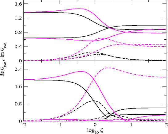
Figure 1: (Color online) The real (solid lines) and imaginary (dashed lines) parts of the first order even-parity modes as functions of the drag-to-lift ratio $\zeta$. The heavy and light lines correspond to $\zeta^{\prime}=0$ and $\zeta^{\prime}=\zeta$ cases. The upper and lower panels correspond to the rotation frequencies $\Omega/\omega_{\perp}=0.36$ and $\Omega/\omega_{\perp}=0.9$, respectively. The frequencies are in units of $\omega_{\perp}$.

The real (solid lines) and imaginary (dashed lines) parts of the first order even-parity modes as functions of the drag-to-lift ratio $\zeta$ are shown in Fig. 1. The frequencies are in units of $\omega_{\perp}$. The parameter values are those in the MIT experiment MIT1 : $\omega_{3}^{2}/\omega_{\perp}^{2}=0.057$ and we assumed that the overlap volume corresponding to $\epsilon=0.5$ and the condensate fraction is $20\%$ which implies $f=1.125$. The two panels in Fig. 1 are representative for the slow and fast rotation limits with the values of the spin frequency $\Omega/\omega_{\perp}=0.36$ (as is the case in the experiment MIT1 ) and $\Omega/\omega_{\perp}=0.9$. The heavy and medium lines correspond to the cases $\zeta^{\prime}=0$ and $\zeta=\zeta^{\prime}$, respectively. The generic features of the modes (seen also for more complicated cases below) are the asymptotically constant values of the real and the vanishing of the imaginary parts, except for the case of $\zeta=\zeta^{\prime}$ and strong-coupling ($\zeta\gg 1$) where the damping tends to a constant value asymptotically. The mode crossing occurs when the condition $\tilde{\beta}^{\prime}=1$ is fulfilled. This can be seen directly from the characteristic equations: the real and imaginary parts degenerate to a single value since for $\tilde{\beta}^{\prime}=1$ the first term on right hand side of Eq. (27) and the phase of the second term in Eq. (27) vanish. The position of the mode crossing when $\zeta^{\prime}=0$ and $\zeta^{\prime}=\zeta$ is different. The reason is that while the mode crossing is still defined by the condition $\tilde{\beta}^{\prime}=1$, the functional dependence of $\zeta$ on $\tilde{\beta}^{\prime}$ for $\zeta^{\prime}=0$ and $\zeta^{\prime}=\zeta$ changes. The damping of the modes has two maxima, one at the position of the mode crossing, the second at $\zeta=1$.

In the weak-coupling limit $(\zeta\ll 1$) the splitting in the real parts of the modes is twice the rotation frequency consistent with Eq. (28) and the centroid is at ${\rm Re}~{}\sigma_{\rm eve}=\omega_{\perp}$. In the strong-coupling limit $(\zeta\gg 1$) the splitting would have been absent if the fluids were to occupy the same volume (i.e., $\beta^{\prime}=\tilde{\beta}^{\prime}=1$ when $\zeta\to\infty$). The strong-coupling expansion (30) to next-to-leading order in $\delta\ll 1$ reads

$${\rm Re}~{}\sigma_{\pm}\to\pm\sqrt{\omega_{\perp}^{2}-\Omega^{2}}\pm\Omega\delta+{\cal O}(\zeta^{-2})+{\cal O}(\delta^{2}).$$ (32)

Thus, the splitting of the real parts of the modes in the strong coupling regime is a direct measure of the renormalization of the $\beta^{\prime}$ coefficient due to the mismatch of the volumes of the condensate and the thermal cloud (provided the ratio $\rho_{S}/\rho_{N}$ is known). The centroid of the splitting is defined by the first term in Eq. (32). The overall behavior of the modes in the fast (or near critical, $\Omega/\omega_{\perp}\leq 1$) rotation regime, shown in the lower panel of Fig. 1, is qualitatively the same as for the slow rotations. The splittings of the real parts of the modes increases in the strong and weak coupling limits linearly with $\Omega$. In the fast rotation regime, the modes are either partially (for $\zeta^{\prime}=0$) or fully (for $\zeta^{\prime}=\zeta$) damped in the strong-coupling limit. Note that the point where the modes cross is independent of $\Omega$.

III.2 second-order harmonic oscillations

This section contains a formal derivation of the characteristic equations for $l=2$ modes in the inviscid and viscose normal-fluid cases. The numerical results and the physical properties of these modes are discussed in the following section.

III.2.1 Inviscid limit

It is instructive to consider the second-order harmonic small-amplitude oscillations first in the inviscid limit ($\nu\to 0$). The characteristic equations for the second-order center of mass and relative oscillations modes are

$$\sigma^{2}V_{i;j}+(\Omega^{2}-\omega_{i}^{2})V_{ij}+2i\epsilon_{ilm}\Omega_{m}\sigma V_{l;j}$$

$$-\Omega_{i}\Omega_{k}V_{kj}+\delta_{ij}\delta\Pi^{(+)} = 0,$$ (33)

$$\sigma^{2}U_{i;j}+(\Omega^{2}-\omega_{i}^{2})U_{ij}+2i\epsilon_{ilm}\Omega_{m}\sigma U_{l;j}$$

$$-2i\Omega\tilde{\beta}_{ik}\sigma U_{k;j}-\Omega_{i}\Omega_{k}U_{kj}+\delta_{ij}\delta\Pi^{(-)} = 0,$$ (34)

and the even and odd-parity modes can be treated separately. Equation (III.2.1) for center of mass oscillations differs from the analogous Eq. (11) of Paper I by the variation of the pressure tensor $\delta_{ij}\delta\Pi^{(+)}$; since the transverse-shear ($l=2$ and $|m|=1$) and the toroidal ($l=2$ and $|m|=2$) modes do not involve this quantity, these modes are identical to those derived earlier, see Eqs. (1) and (I). The quasi-radial pulsation modes couple the center of mass and relative oscillations and will be examined below.

We start with the toroidal modes of relative oscillations, which are governed by the equations

$$\left[\sigma^{2}-2i\Omega\tilde{\beta}\sigma-2(\omega_{\perp}^{2}-\Omega^{2})\right](U_{11}-U_{22})$$

$$+4i\Omega(1-\tilde{\beta}^{\prime})\sigma U_{12} = 0,$$ (35)

$$\left[\sigma^{2}-2i\Omega\tilde{\beta}\sigma-2(\omega_{\perp}^{2}-\Omega^{2})\right]U_{12}$$

$$-i\Omega(1-\tilde{\beta}^{\prime})\sigma(U_{11}-U_{22}) = 0.$$ (36)

The associated characteristic equation and the solutions are identical to Eq. (26) and (27), respectively, if we replace in these equations the radial trapping frequency by $\omega_{\perp}^{*2}=2\omega_{\perp}^{2}-\Omega^{2}$; clearly, with the substitution above, the limiting behavior of the modes for large and small frictions are the same as for the first order harmonic modes. The transverse-shear (odd-parity) modes are given by the components of Eq. (34) for the tensors $U_{i;3}$ and $U_{i3}$, $i=1,2$:

$$(\sigma^{2}-2i\Omega\tilde{\beta}\sigma)U_{1;3}+2i\Omega(1-\tilde{\beta}^{\prime})\sigma U_{2;3}$$

$$-(\omega_{\perp}^{2}-\Omega^{2})U_{13} = 0,$$

$$(\sigma^{2}-2i\Omega\tilde{\beta}^{\prime\prime}\sigma)U_{1;3}+(\sigma^{2}-2i\Omega\tilde{\beta}^{\prime\prime}\sigma-\omega_{3}^{2})U_{13} = 0,$$

and the remaining two equations are obtained from Eqs. (III.2.1) and (III.2.1) via the $1\leftrightarrow 2$ interchange. The corresponding characteristic equation is of order 7.

By a suitable combination of the even-parity components of Eq. (III.2.1) we find the following set of equations for the virial combinations $V_{11}+V_{22}$, $V_{1;1}-V_{2;2}$, and $V_{33}$ describing the pulsation modes

$$\left(\sigma^{2}/2-\omega_{\perp}^{2}+\Omega^{2}\right)+\left(V_{11}+V_{22}\right)$$

$$-2i\Omega\sigma(V_{1;2}-V_{2;1})-\left(\sigma^{2}-2\omega_{3}^{2}\right)V_{33} = 0,$$ (39)

$$\sigma^{2}(V_{1;2}-V_{2;1})+i\Omega\sigma(V_{11}+V_{22}) = 0,$$ (40)

$$(\sigma^{2}-2\omega_{3}^{2})V_{33}+2\delta\Pi^{(+)} = 0,$$ (41)

where the tensor $\delta\Pi^{(+)}$ is defined by Eq. (B10) of the Appendix B. It involves the same set of virials and, in addition, couples these equations to the virials describing relative motions. Analogous manipulations on Eq. (34) lead to

$$\left(\sigma^{2}/2-i\Omega\tilde{\beta}\sigma-\omega_{\perp}^{2}+\Omega^{2}\right)(U_{11}+U_{22})-\left(\sigma^{2}-2i\Omega\tilde{\beta}^{\prime\prime}\sigma-2\omega_{3}^{2}\right)U_{33}-2i\Omega(1-\tilde{\beta}^{\prime})\sigma(U_{1;2}-U_{2;1}) = 0,$$ (42)

$$(\sigma^{2}-2i\Omega\tilde{\beta}\sigma)(U_{1;2}-U_{2;1})+i\Omega(1-\tilde{\beta}^{\prime})\sigma(U_{11}+U_{22}) = 0,$$ (43)

$$(\sigma^{2}-4i\Omega\tilde{\beta}^{\prime\prime}-2\omega_{3}^{2})U_{33}+2\delta\Pi^{(-)} = 0,$$ (44)

with $\delta\Pi^{(-)}$ defined by Eq. (B11) of the Appendix B. The resulting characteristic equations for the quasiradial pulsation modes ($l=2$, $m=0$) is of order 9.

III.2.2 Including viscosity of thermal cloud

The kinematic viscosity of the normal-fluid can be included in the tensor virial formalism perturbatively and the Eulerian variations of the viscose stress tensor are computed in the Appendix B. The virial equation that contain the second-order harmonic $l=2$ and $-2\leq m\leq 2$ modes in the presence of normal cloud viscosity are obtained upon substituting Eq. (B3) of the Appendix B in Eqs. (III.2.1) and (34):

$$\sigma^{2}V_{i;j}+2i\epsilon_{ilm}\Omega_{m}\sigma V_{l;j}+(\Omega^{2}-\omega_{i}^{2})V_{ij}-\Omega_{i}\Omega_{k}V_{kj}+\delta_{ij}\delta\Pi^{(+)}$$

$$-\frac{5i\nu\sigma}{1+f}\left(\frac{V_{i;j}}{\bar{a}_{j}^{2}}+\frac{V_{j;i}}{\bar{a}^{2}_{i}}-\frac{V_{ll}}{3\bar{a}_{l}^{2}}\delta_{ij}\right)+\frac{5i\nu\sigma}{1+f}\left(\frac{U_{i;j}}{\bar{a}_{j}^{2}}+\frac{U_{j;i}}{\bar{a}^{2}_{i}}-\frac{U_{ll}}{3\bar{a}_{l}^{2}}\delta_{ij}\right) = 0,$$ (45)

$$\sigma^{2}U_{i;j}+2i\epsilon_{ilm}\Omega_{m}\sigma U_{l;j}+(\Omega^{2}-\omega_{i}^{2})U_{ij}-\Omega_{i}\Omega U_{kj}+\delta_{ij}{\delta\Pi}^{(-)}-2i\Omega\tilde{\beta}_{ik}\sigma U_{k;j}$$

$$+\frac{5if\nu\sigma}{1+f}\left(\frac{V_{i;j}}{\bar{a}_{j}^{2}}+\frac{V_{j;i}}{\bar{a}^{2}_{i}}-\frac{V_{ll}}{3\bar{a}_{l}^{2}}\delta_{ij}\right)-\frac{5if\nu\sigma}{1+f}\left(\frac{U_{i;j}}{\bar{a}_{j}^{2}}+\frac{U_{j;i}}{\bar{a}^{2}_{i}}-\frac{U_{ll}}{3\bar{a}_{l}^{2}}\delta_{ij}\right) = 0.$$ (46)

Note that Eqs. (45) and (46) are symmetric with respect to the simultaneous interchanges $U\leftrightarrow V$, $f\nu\leftrightarrow\nu$ and $\delta\Pi^{(-)}\leftrightarrow\delta\Pi^{(+)}$, however Eq. (46) contains a term $\propto\beta_{ik}$ which is absent in Eq. (45). To keep the presentation compact we will quote below only the components of Eq. (46); the analogous components of Eq. (45) follow by the interchanges above and by setting $\beta_{ij}=0$ (this will be abbreviated as the $UV$-transformation).

The transverse-shear modes are determined by the eight components of the Eqs. (45) and (46) which are odd in index 3, i.e., $V_{3;i}$, $V_{i;3}$, $U_{3;i}$ and $U_{i;3}$, where $i=1,2$. The odd equations for the virials describing the relative motions are

$$\left(\sigma^{2}-2i\Omega\tilde{\beta}\sigma+i\chi f\nu\sigma\right)U_{1;3}-\left(\omega_{\perp}^{2}-\Omega^{2}+if\nu\sigma\right)U_{13}+2i\Omega(1-\tilde{\beta}^{\prime})\sigma U_{2;3}-i\chi f\nu\sigma V_{1;3}+if\nu\sigma V_{13} = 0,$$ (47)

$$\left(\sigma^{2}-2i\Omega\tilde{\beta}^{\prime\prime}\sigma-\omega_{3}^{2}-if\nu\sigma\right)U_{13}+\left(\sigma^{2}-2\Omega i\tilde{\beta}^{\prime\prime}\sigma-i\chi f\nu\sigma\right)U_{1;3}+if\nu\sigma V_{13}-i\chi f\nu\sigma V_{1;3} = 0,$$ (48)

two additional equations are obtained from Eqs. (47) and (48) via the $1\leftrightarrow 2$ interchange and the analogous equations for the center of mass virials are obtained via the $UV$ transformation.

Here $\chi\equiv 1-\bar{a}_{1}^{2}/\bar{a}_{3}^{2}$ and $\nu^{\prime}=5\nu/\bar{a}_{1}^{2}(1+f)$ and the primes have been dropped in the equations. (Note that we used the relation $U_{ij}=U_{i;j}+U_{j;i}$ to manipulate the components of Eq. (46) to the form above.) The resulting two sets of equations for the center of mass and the relative virials decouple in the limit $\nu\to 0$, as they should. The dissipation in the first set is driven by the viscosity of the normal-fluid. In the second set the normal-fluid viscosity contributes to the damping of the Lagrangian displacements which are orthogonal to those damped by the mutual friction, and in addition, the mutual friction damping time scale is renormalized form $2\Omega\tilde{\beta}$ to $2\Omega\tilde{\beta}+(1-\chi)f\nu$; (this renormalization vanishes for a sphere, since then $\chi=1$). The resulting characteristic equation is of order 12.

The toroidal modes are determined by the even in index 3 components of Eqs. (34) and (III.2.1) written for the virials $V_{i;i}$, $V_{i;j}$, $U_{i;i}$ and $U_{i;j}$, where $i,j=1,2$. These equations can be manipulated to a set of four equations and those for the relative virials are

$$\left[\sigma^{2}-2i\Omega\tilde{\beta}\sigma-2if\nu\sigma-2(\omega_{\perp}^{2}-\Omega^{2})\right](U_{11}-U_{22})+4i\Omega(1-\tilde{\beta}^{\prime})\sigma U_{12}+2if\nu\sigma(V_{11}-V_{22}) = 0,$$ (49)

$$\left[\sigma^{2}-2i\Omega\tilde{\beta}\sigma-2if\nu\sigma-2(\omega_{\perp}^{2}-\Omega^{2})\right]U_{12}-\Omega(1-\tilde{\beta}^{\prime})i\sigma(U_{11}-U_{22})+2if\nu\sigma V_{12} = 0,$$ (50)

the analogous equations for the center of mass virials follow by the $UV$ transformation. As above, the effect of the kinematic viscosity is the coupling of the center of mass and relative modes and the renormalization of the damping due to the mutual friction $\Omega\tilde{\beta}\to\Omega\tilde{\beta}+\nu$. The corresponding characteristic equations is of eighth order.

The pulsation modes are determined by the equations which are even in index 3. For incompressible ellipsoids these should be supplemented by the conditions of vanishing of the divergence of perturbations of each fluid [Paper I, Eq. (38) and its analog for the $U_{ii}$ virials]. We shall proceed directly to the compressible fluid case. Combining the equations for the virials $V_{i;i}$, $V_{i;j}$, $U_{i;i}$ and $U_{i;j}$, where $i=1,2,3$ and $j=1,2$, we find two (coupled) subsets of equations, the first involving perturbations which are orthogonal to the spin axis

$$(\sigma^{2}-2i\Omega\tilde{\beta}\sigma)(U_{1;2}-U_{2;1})+i\Omega(1-\tilde{\beta}^{\prime})\sigma(U_{11}+U_{22}) = 0,$$ (51)

and the second subset which couples the orthogonal to the spin parallel perturbations [$\tilde{\nu}\equiv(1-\chi)\nu]$

$$\left(\frac{\sigma^{2}}{2}-if\nu\sigma-i\Omega\tilde{\beta}\sigma-\omega_{\perp}^{2}+\Omega^{2}\right)(U_{11}+U_{22})-2i\Omega(1-\tilde{\beta}^{\prime})\sigma(U_{1;2}-U_{2;1})$$

$$-\left(\sigma^{2}-2i\Omega\tilde{\beta}^{\prime\prime}\sigma-2\omega_{3}^{2}-2if\tilde{\nu}\sigma\right)U_{33}+if\nu\sigma(V_{11}+V_{22})+2if\tilde{\nu}\sigma V_{33} = 0,$$ (52)

$$\left(\frac{\sigma^{2}}{2}-\frac{2i}{3}f\tilde{\nu}\sigma-i\Omega\beta^{\prime\prime}\sigma-\omega_{3}^{2}\right)U_{33}+\frac{i}{3}f\nu\sigma(U_{11}+U_{22})+\delta\Pi^{(-)}+\frac{2i}{3}f\tilde{\nu}\sigma V_{33}-\frac{i}{3}f\nu\sigma(V_{11}+V_{22}) = 0,$$ (53)

Note that the kinematic viscosity renormalizes the damping along the spin axis as $\Omega\tilde{\beta}^{\prime\prime}\to\Omega\tilde{\beta}^{\prime\prime}+(1-\chi)\nu$ and in the plane orthogonal to the spin axis as $\Omega\tilde{\beta}\to\Omega\tilde{\beta}+\nu$. Unlike the $m\neq 0$ modes, the center of mass and relative motions remain coupled in the limit $\nu\to 0$ due to the differences in the pressure perturbations of the superfluid and normal-fluid. The characteristic equation for the pulsation modes is of order 9.

III.3 Numerical solutions

The fluid oscillations can be characterized in terms of Lagrangian displacement fields. For a single fluid, the $l=2$ displacement fields are shown schematically in Fig. 2 for (top-to-bottom) $m=1$, $m=2$, and $m=0$ modes. The $m=\pm 1$ modes are antisymmetric with respect to the body rotation plane and involve relative shearing of the “northern” and “southern hemisphere”. The $m=\pm 2$ modes are non-axisymmetric, i.e., they tend to break the axial symmetry of the body by deforming them into triaxial form. The $m=0$ modes are symmetric with respect to the body rotation plane and are the generalization of the ordinary pulsations of a sphere to the rotation.

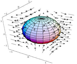
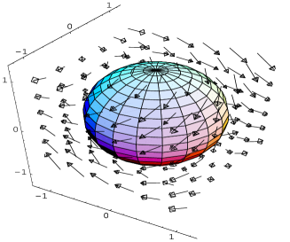
Figure 2: (Color online) Schematic illustration of the displacement fields for $l=2$ and (top-to-bottom) $m=1$, $m=2$, and $m=0$ oscillation modes. The rotation vector is along the vertical $z$ axis and is directed from the “south” to the “north pole”.

In the two fluid setting, the superfluid and normal-fluid motions can be visualized in terms of either the two “proper”displacements $\bm{\xi}_{S,N}$ [defining the $V_{S,N}$ virials, Eq. (18)] or by their linear superpositions $\bm{\xi}_{+}=(\bm{\xi}_{N}+\bm{\xi}_{S})$, $\bm{\xi}_{-}=(\bm{\xi}_{-}-f\bm{\xi}_{N})$ [defining the $V$ and $U$ virials, Eqs. (19) and (20)]. Note that the displacement fields and, hence, their linear superpositions, are linear in coordinates and the vector fields in Fig. 2 can be associated with either displacement above; (of course, the coefficients in the generic relation $\xi_{i}=L_{ij}x_{j}$ are different in each case). The relative oscillations can be viewed as a superposition of two antiparallel displacement fields $\bm{\xi}_{S,N}$ each following the patterns shown in Fig. 2 and, thus, involving countermotions of the two fluids. Similarly, the center of mass modes are a superposition of the parallel displacement fields of the fluids and correspond to a comotion of the fluids.

We now turn to the numerical solutions of the characteristic equations for the second-order virials. The results shown below were obtained for the parameter values $\omega_{3}^{2}/\omega_{\perp}^{2}=0.057$, $f=1.125$. (The latter corresponds to the overlap volume $\epsilon=0.5$ and the condensate fraction $20\%$)

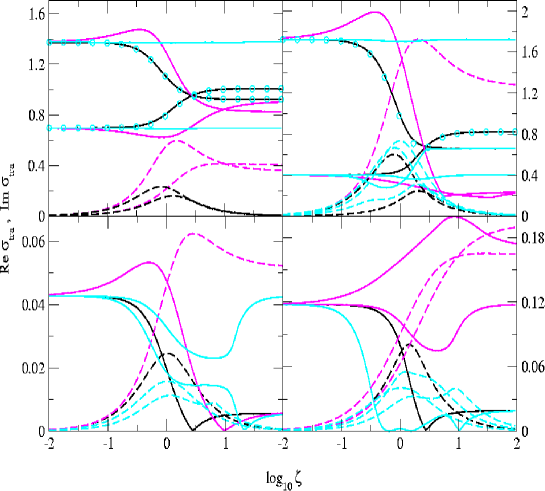
Figure 3: (Color online) The dependence of the second-order transverse-shear ($l=2$ $m=\pm 1$) modes on the drag-to-lift ratio $\zeta$; the real and imaginary parts are shown by the solid and dashed lines. The heavy and the medium lines correspond to the cases $\zeta^{\prime}=0$ and $\zeta^{\prime}=\zeta$ with $\nu=0$. The light lines show the modes for $\nu=2\Omega\beta$ and $\zeta^{\prime}=0$. The rotation frequency is $\Omega/\omega_{\perp}=0.36$ in the left panels and $\Omega/\omega_{\perp}=0.72$ in the right panels; the top and bottom panels show the high and the low frequency modes, respectively. The circles show the viscose modes that coincide with the modes in the inviscid limit.

Fig. 3 shows the real (solid lines) and imaginary (dashed lines) parts of the second-order transverse-shear modes ($l=2,m=\pm 1$). The heavy lines correspond to the inviscid case with $\zeta^{\prime}=0$; the medium lines correspond to the inviscid case but with $\zeta^{\prime}=\zeta$, and the light lines - to the viscous normal-fluid case with $\zeta^{\prime}=0$. The coefficient $\beta^{\prime\prime}$ is set equal to zero everywhere. The left and right panels correspond to the rotation frequencies $\Omega/\omega_{\perp}=0.36$ and $\Omega/\omega_{\perp}=0.72$. The characteristic equation for the transverse-shear modes is of order 7, however the solutions appear as complex-conjugate pairs, i.e., there are only three distinct solutions plus a zero-frequency mode; this mode degeneracy reflects the axial symmetry of the problem. An interesting feature seen in the inviscid limit, e.g., when $\zeta^{\prime}=0$, is the mode crossing at $\tilde{\beta}^{\prime}=1$, where the real and imaginary parts of the two high-frequency modes coincide and the real part of the third low-frequency mode vanishes. The mode crossing occurs because the terms $\propto 1-\tilde{\beta}^{\prime}$ in Eq. (III.2.1) and its analog equation under the $1\leftrightarrow 2$ replacement vanish, i.e., these equations become invariant under the exchange of the indices 1 and 2. Nonzero $\zeta^{\prime}$ causes a shift in the value of $\zeta$ where the modes cross, which is a simple consequence of the different functional dependence of $\zeta$ on $\tilde{\beta}^{\prime}$ for the cases $\zeta^{\prime}=0$ and $\zeta^{\prime}=\zeta$. Note that the crossover from the weak- to the strong-coupling regime is monotonic for the case $\zeta^{\prime}=0$ while the functions acquire maximum or minimum at intermediate values of $\zeta$ when $\zeta^{\prime}\neq 0$. The asymptotics of the real and imaginary parts of the transverse-shear modes are the same as for the first-order even-parity modes (Fig. 1): the real parts of the modes tend asymptotically to constant values and the imaginary parts vanish except for the case $\zeta=\zeta^{\prime}$ and strong-coupling ($\zeta\gg 1$) where the damping tends to a constant value asymptotically. The splitting of the modes is twice the rotation frequency in the weak-coupling regime and is proportional to $f\Omega$ in the strong-coupling regime, where $f$, defined via the relation $\tilde{\beta}^{\prime}=(1+f)\beta^{\prime}$, reflects the mismatch in the volume of the normal-fluid and superfluid. The damping of the modes is negligible in the limits of both large and small $\zeta$ (except $\zeta^{\prime}=\zeta$ and $\zeta\to\infty$ limit) and is maximal for $\zeta\sim 1$. This feature is generic to the damping of all modes and is a result of low vortex mobility for motions away or towards the spin axis: in the small $\zeta$ limit the lattice moves with the superfluid; in the large $\zeta$ limit it is locked to the normal-fluid. Comparing the modes for the slow and fast rotation cases (left and right panels of Fig. 3) reveals the following differences: (i) the splittings of the real parts of the modes are larger in the strong- and weak-coupling limits consistent with the linear scalings with $\Omega$; (ii) the two high-frequency modes are nonoscillatory in the crossover region $\zeta\sim 1$.

When the viscosity of the normal-fluid is taken into account, the number of modes double, since the relative and center of mass modes mix. The solutions of the 12th order characteristic equation for the transverse-shear modes in the case of viscous thermal cloud are shown in Fig. 3 by light lines. The value of the kinematic viscosity is fixed at $\nu=2\beta\Omega$. (We note here that the parameter $\nu/\beta\Omega$ is not small in our examples below, and the perturbation expansion for the relative modes breaks down for $\nu/\beta\Omega\sim 1$. The quoted value was chosen to make the differences between the inviscid and viscous case visible on the scale of the figure.) The solutions to the secular equations for the modes appear as complex-conjugates (reflecting the axial symmetry of the problem), i.e., there are six distinct solutions for the transverse-shear modes. Consistent with the perturbative treatment of the viscosity effects a subset of modes in Fig. 3 shows only small deviations from the inviscid case, mostly in the crossover region between the strong and weak-couplings ($\zeta\sim 1$). The remainder modes are almost independent of the mutual friction and are associated with the center of mass oscillations modes. The generic features of the relative oscillation modes are unchanged when viscosity is included (the mode-crossing, asymptotic splittings of the real parts and the asymptotic decay of the imaginary parts). The shift in the position of the crossing point compared to the inviscid and $\zeta^{\prime}=0$ case is due to the rescaling of the $\tilde{\beta}^{\prime}$ parameter by the terms $\propto\chi\nu$. Note that the damping of the center of mass modes is solely due to the viscosity and the bell-shaped imaginary parts seen in Fig. 2 are the consequence of our assumption that $\nu\propto\beta$ (assigning a constant value to the kinematic viscosity would not change the qualitative picture above, but would render the damping of the center of mass oscillations independent of $\zeta$).

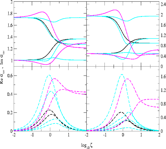
Figure 4: (Color online) The dependence of the second-order toroidal ($l=2$ $m=\pm 2$) modes on the drag-to-lift ratio $\zeta$. The left and right panels correspond to $\Omega/\omega_{\perp}=0.36$ and $\Omega/\omega_{\perp}=0.72$. The labeling conventions are the same as in Fig. 3.

The solutions of the fourth-order characteristic equation for the toroidal modes ($l=2,m=0$) are displayed in Fig. 4 (conventions are the same as in Fig. 3). Only two distinct solutions exist in the inviscid limit, since the modes appear as complex-conjugates due to the axial symmetry. Since the main properties of the toroidal modes are similar to those of the transverse-shear modes we only briefly list these features: (i) the pair of solutions degenerate to a single value (mode-crossing) for $\tilde{\beta}^{\prime}=1$ in the $\zeta^{\prime}=0=\nu$ limits, since then Eqs. (III.2.1) and (III.2.1) become identical. (ii) For $\zeta^{\prime}=\zeta$ the value of $\zeta$ at which the crossing occurs shifts to larger values. (iii) The real parts of the modes are asymptotically constant; the two imaginary parts decay asymptotically to zero and are maximal at ${\rm log}_{10}\zeta=0$ and at the mode-crossing point, respectively. (iv) For $\zeta=\zeta^{\prime}$ the imaginary parts are constants in the limit $\zeta\to\infty$. The asymptotic values of the frequencies of the toroidal modes are numerically larger that those of the transverse-shear modes. In the viscose case the mixing of the modes doubles the number of distinct toroidal modes and the additional modes can be attributed to the center of mass oscillations. The deviation of the modes from the inviscid case are small in Fig. 4 and the perturbative treatment of the viscous effects is justified.

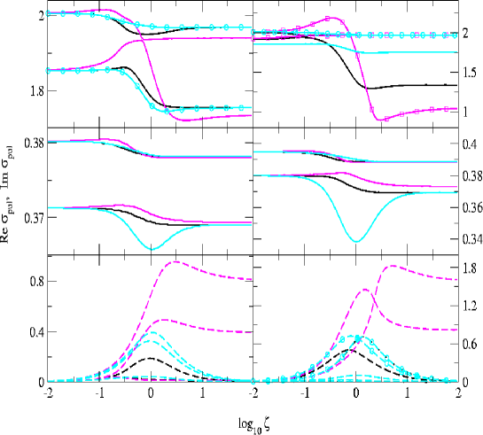
Figure 5: (Color online) The dependence of the second-order pulsation ($l=2$ $m=\pm 0$) modes on the drag-to-lift ratio $\zeta$. The left and right panels correspond to $\Omega/\omega_{\perp}=0.36$ and $\Omega/\omega_{\perp}=0.72$. The labeling conventions are the same as in Fig. 3 (the circles and squares show the modes in the viscose case which coincide with those in the inviscid limit).

Figure 5 displays the real and imaginary parts of the pulsation ($l=2$ $m=0$) modes. The distinctive feature of the pulsation modes is that the center of mass and relative oscillations mix even in the inviscid limit because pressure perturbations for the normal-fluid and the condensate are governed by different adiabatic indices. The ninth-order secular equation for the pulsation modes has four distinct solutions plus a zero-frequency mode (as before, because of the axial symmetry the modes appear as complex-conjugates). Unlike the modes with $m\neq 0$ there is no generic crossing point for the pulsation modes. Including the viscosity of the thermal cloud causes small modifications in the oscillations modes (but does not change their overall number). The modes are mostly affected in the crossover regime $\zeta\sim 1$ because of our assumption $\nu\propto\beta$. The asymptotic behavour of the damping of the modes is the same as for the transverse-shear and toroidal modes.

IV Conclusions and summary

The analysis above shows that the finite temperature oscillation modes of a harmonically confined rotating Bose-Einstein gas contain rich information on the physics of condensate, the thermal cloud and their interactions via the vortex lattice. The features of the oscillation modes are summarized below.

The modes separate into two classes corresponding to the center of mass and relative oscillations of the thermal cloud and the condensate. The first class of modes involves oscillations of the combined mass of the cloud and the condensate, and is the analog of the first sound in nonrotating superfluids. The second class of modes carries zero net mass-current, involves entropy oscillations of the thermal cloud, and hence, is the analog of the second sound.

The two classes of modes are independent when the normal cloud is inviscid. An exception are the radial pulsations, which are coupled due to the difference in adiabatic pressure perturbations of the cloud and the condensate. If the thermal cloud is viscous, the center of mass and relative oscillations are coupled for all types of modes.

Two distinct mechanisms of damping of perturbations from the equilibrium rotating state are operative: the mutual friction between the condensate and the thermal cloud, mediated by the vortex lattice, damps the relative oscillations. The kinematic viscosity damps the center of mass oscillations of the thermal cloud. When the two classes of modes are coupled, the kinematic viscosity renormalizes the damping of the relative oscillation modes.

First order harmonic oscillations. At finite temperatures the lowest-order non-trivial (i.e., different from ordinary rotation) modes of oscillations belong to the first order ($l=1$) harmonics. These modes represent relative oscillations of the thermal cloud and are described by our Eqs. (26) and (27). According to Eq. (26) the eigenmodes of the odd-parity oscillations should coincide with $\omega_{z}$ with zero damping unless there is nonzero friction orthogonal to the equatorial plane (which would indicate convective motions or vortex bending). The even-parity modes are described by Eq. (27) and they carry information on a number of macroscopic and microscopic parameters. For example, locating experimentally the crossing point of the two eigenmodes (see Fig. 1) would fix the value of the $\zeta$ parameter, provided the force component proportional to $\zeta^{\prime}$ is negligible. Measuring in addition the position of the centroid around which the modes are split in the strong-coupling regime ($\zeta\gg 1$) would fix both $\zeta$ and $\zeta^{\prime}$ parameters. The magnitude of the splitting in the strong-coupling regime, provides information on the volume filling factor and the fractional densities of the condensate and the cloud. If the Iordansky force is operative the damping of the modes in the strong-coupling regime would be significantly affected (asymptotically constant, instead of going to zero, see Fig. 1).

second-order harmonic oscillations. These oscillations are more complex, since they involve a larger number of modes and the center of mass and relative oscillations can be coupled. The features of the relative transverse-shear ($m=\pm 1$) and toroidal ($m=\pm 2$) modes are as follows. The condition $\tilde{\beta}=1$ defines a mode crossing point for the high-frequency modes. The real parts of the modes are asymptotically constant and the imaginary parts tend to zero as $\zeta\to\pm\infty$, except when $\zeta^{\prime}\sim\zeta$ and $\zeta\to\infty$, in which case the imaginary parts tend to constants. The bell-shaped form of the imaginary parts with maxima at ${\rm log}_{10}~{}\zeta=0$ and ${\rm log}_{10}~{}\zeta=0.4$ (for $\zeta^{\prime}=0$) is generic to the relative transverse-shear ($m=\pm 1$) and toroidal ($m=\pm 2$) modes. Increasing the rotation frequency enhances the damping of the modes (left/right panels of Figs. 3-5) since the dissipation scales linearly with the spin frequency. The asymptotic splitting of the eigenmodes in the strong- and weak-coupling limits is enhanced linearly in $\Omega$. The distinctive feature of the second-order harmonic pulsation modes ($m=0$) is that they couple the relative and center of mass oscillations even when the viscosity of the matter is negligible. There is no mode crossing for the pulsation modes (for the common case $\zeta^{\prime}=0$) and the damping has its maxima at $\zeta=0$ only.

Implications for experiments. The drag-to-lift ratios depend on the elementary processes of quasi-particle–vortex scattering, the strength of the interparticle interactions, and on thermodynamic parameters, such as the density and the temperature. Note that the $l=0,\pm 2$ modes of a rotating Bose gas have been measured experimentally at zero-temperature and are consistent with results quoted in the Introduction. A possible scenario of mapping out the dependence of the modes on the mutual friction parameters could involve tuning the interparticle interactions in the vicinity of a Feshbach resonance and sizably changing the quasi-particle–vortex scattering cross section by small variations in the magnetic field. Varying the thermodynamic parameters, for example, the temperature of the system is another possibility. If the system is prepared (or the bosonic species are chosen) such that the strong-coupling regime is operative, measuring the relative oscillations modes at various spin frequencies can provide information on the actual values of the mutual friction and related parameters. The mutual friction coefficients can also be fixed by measuring the damping of the modes, in particular the strong-coupling limit discriminates the case where the Iordansky force is operative. Experimental studies of the dependence of the second-order harmonic modes on the lift-to-drag ratios and the variations of the spin-frequency, apart from fixing the parameters reflecting the microphysics of quasi-particle–vortex interactions can, in addition, provide information on the magnitude of the kinematic viscosity from the damping or splitting of the eigenfrequencies of the center of mass modes. We remind that Eqs. (1)-(I) for the center of mass modes remain valid at finite temperatures whenever these are decoupled from the relative oscillations (e.g. the $\nu\to 0$ limit).

Other systems. The method described above could be applied to superfluid Fermi systems at finite temperatures with minor modifications. For Fermi superfluids which rotate as a rigid body and are confined by a harmonic trap, the oscillation modes will differ from those described above to the extent the equations of states of the normal and superfluid differ from those of a Bose gas. Since the linearized perturbation equations involve pressure perturbations only for the pulsation modes, the remainder oscillations would be identical to those described above. The pulsation modes can be easily handled by using an appropriate adiabatic index for a Fermi-superfluid at finite temperatures.

Appendix A Virial equations for uniform rotations

Taking the moment of Eq. (7) with weight 1 and integrating over $V_{\alpha}$ we obtain the first order virial equation

$${d\over dt}\int_{V_{\alpha}}{d^{3}x\rho_{\alpha}u_{{}_{\alpha},i}}=2\epsilon_{ilm}\Omega_{m}\int_{V_{\alpha}}{d^{3}x\rho_{\alpha}u_{{}_{\alpha}l}}$$

$$+(\Omega^{2}\delta_{ij}-\omega_{i}^{2})I_{\alpha,i}-\Omega_{i}\Omega_{j}I_{\alpha,i}+\int_{V_{\alpha}}d^{3}xF_{\alpha\beta,i},$$ (54)

where

$$I_{\alpha,i}=\int_{V_{\alpha}}{d^{3}x\rho_{\alpha}x_{i}}$$ (55)

is the moment of inertia of fluid $\alpha$, and we used a boundary condition which assumes that the projection of the stress

$$-p_{\alpha}\delta_{ik}+\delta_{\alpha,N}P_{ik},\quad\alpha=S,N$$

orthogonal to a bounding surface vanishes in equilibrium (the free-surface condition).

Taking the first moment of Eq. (7) with weight $x_{i}$ and integrating over the volume $V_{\alpha}$ results in the second-order virial equation

$${d\over dt}\int_{V_{\alpha}}{d^{3}x\rho_{\alpha}x_{j}u_{\alpha,i}}=2{\cal T}_{{\alpha},ij}+\delta_{ij}\Pi_{\alpha}+\delta_{\alpha,N}{\cal P}_{ij}$$

$$+(\Omega^{2}-\omega_{i}^{2})I_{{\alpha},ij}+2\epsilon_{ilm}\Omega_{m}\int_{V_{\alpha}}{d^{3}x\rho_{\alpha}x_{j}u_{\alpha,l}}$$

$$-\Omega_{i}\Omega_{k}I_{{\alpha},kj}+\int_{V_{\alpha}}d^{3}xx_{j}F_{\alpha\beta,i},$$ (56)

where

$$I_{{\alpha},ij}\equiv\int_{V_{\alpha}}{d^{3}x\,\rho_{\alpha}x_{i}x_{j}},\quad\delta_{ij}\Pi_{\alpha}\equiv\delta_{ij}\int_{V_{\alpha}}d^{3}x\,p_{\alpha},$$

$${\cal T}_{{\alpha},ij}\equiv{1\over 2}\int_{V_{\alpha}}{d^{3}x\rho_{\alpha}u_{\alpha,i}u_{\alpha,j}},\quad{\cal P}_{ij}=\int_{V_{N}}d^{3}xP_{ij},$$

are the second rank tensors of moment of inertia, pressure, kinetic energy and stress; note that the last tensor is nonzero only in the volume of the thermal cloud and the integration over the mutual friction force $F_{\alpha,\beta}$ in Eq. (56) is over the overlap volume of the normal cloud and the condensate.

For uniformly rotating condensate and thermal cloud the stationary second-order virial equations define the equilibrium forms of the rotating system; we find

$$\Omega^{2}(I_{\alpha,ij}-\delta_{i3}I_{\alpha,3j})-\omega_{i}^{2}I_{\alpha,ij} = -\delta_{ij}\Pi_{\alpha},\quad\alpha=S,N,$$

where the mixture rotates about the $x_{3}$ axis. The diagonal components of these equations provide the equilibrium ratios of the components of the moment of inertia tensor

$$\frac{I_{N,33}}{I_{N,ii}}=\frac{I_{S,33}}{I_{S,ii}}=\frac{\omega_{i}^{2}-\Omega^{2}}{\omega_{3}^{2}},\quad i=1,2.$$ (59)

The moment of inertia tensor of a heterogeneous ellipsoid is

$$I_{\alpha,ij}=\frac{4\pi}{3}a_{\alpha,i}^{3}a_{\alpha,k}a_{\alpha,l}\delta_{ij}\int_{0}^{1}\rho_{\alpha}(m_{\alpha}^{2})m_{\alpha}^{4}dm_{\alpha},$$ (60)

where the density distributions $\rho_{\alpha}(m^{2}_{\alpha})$ are defined in Eqs. (8) and (9). The total mass in the fluid $\alpha$, $M_{\alpha}$ can be related to the moment of inertia tensor by noting that

$$M_{\alpha}=4\pi a_{\alpha 1}a_{\alpha 2}a_{\alpha 3}\int_{0}^{1}\rho_{\alpha}(m_{\alpha}^{2})m_{\alpha}^{2}dm_{\alpha}.$$ (61)

Using Eq. (60) in Eq. (59) we find the ratios of the semi-axis in equilibrium

$$\frac{a_{N,3}}{a_{N,i}}=\frac{a_{S,3}}{a_{S,i}}=\frac{\omega_{i}}{\omega_{3}}\left(1-\frac{\Omega^{2}}{\omega^{2}_{i}}\right)^{1/2},\quad i=1,2.$$ (62)

Despite of the difference in the density profiles of the condensate and the thermal cloud the semi-axis ratios (but not the semiaxis!) are equal; they depend only on the rotation rate and hence are the same for corotating fluids. For axially symmetric figures these conditions place an upper limit on the rotation frequency $\Omega<\omega_{\perp}$. In the nonaxisymmetric case $\Omega<{\rm min}(\omega_{1},\,\omega_{2})$ for fixed $\omega_{1}$ and $\omega_{2}$ or, alternatively, $\omega_{2}>\Omega$ for fixed $\omega_{1}$ at $\Omega<\omega_{1}$. Note that these boundaries correspond to stable solutions under stationary conditions and within the ellipsoidal approximation. Perturbations away from the stability region can result in either dynamically unstable figures that preserve their ellipsoidal structure or (stable) configurations that are not ellipsoids (e.g., the Poincaré’s pear-shaped figures) CHANDRA .

Appendix B Variations of the stress energy and pressure tensors

The variations of the stress tensor, Eq. (11), cannot be expressed in terms of virials in general. This can be done, however, in the perturbative regime, when the effects of viscosity are small. The perturbation expansion about the inviscid limit requires $\sigma_{1}\ll\sigma_{0}$, where $\sigma_{1}$ and $\sigma_{0}$ are the modes in the viscous and inviscid limits. Since the characteristic equations which include fluid viscosity do not permit analytical solutions in general, the validity of the perturbation expansion can be checked numerically (a posteriori) by comparing the values of $\sigma_{0}$ and $\sigma_{1}$ for a fixed mode. Another expansion parameter, that enters only the equations for the relative virials is $\nu/\beta\Omega\ll 1$; the latter condition insures that the modifications of the damping of the modes due to the viscosity are small compared to the inviscid but dissipative (due to the mutual friction) case. The variation of the stress energy tensor in the background equilibrium without internal motions ($\bm{u}=0$) is

$$\delta{\cal P}_{ij}=\nu\int_{V_{N}}\rho_{N}\frac{\partial}{\partial t}\left(\frac{\partial\xi_{N,j}}{\partial x_{i}}+\frac{\partial\xi_{N,i}}{\partial x_{j}}-\frac{2}{3}\frac{\partial\xi_{N,l}}{\partial x_{l}}\delta_{ij}\right)d^{3}x,$$ (63)

Eq. (63) assumes that the kinematic viscosity can be replaced by its average over the profile of the normal cloud, in line with the similar assumption about the mutual friction coefficients.

The perturbative approach expresses the stress energy tensor in terms of Lagrangian displacements corresponding to the inviscid limit (see, e.g., CHANDRA ). For perturbations which are linear in the coordinates, these can be written as

$$\xi_{N,i}=L_{N,i;j}x_{j}$$ (64)

where $L_{N,i;j}$ are nine unknowns which are determined from the solution of the virial equations of second-order in the inviscid limit [no summation over the repeated indices in Eq. (64)]. Using Eqs. (24), (64) in (63) we obtain

$$\delta{\cal P}_{ij}=-i\sigma\nu\int_{V_{N}}\rho_{N}\left(L_{N,i;j}+L_{N,j;i}-\frac{2}{3}\delta_{ij}L_{N,l;l}\right)d^{3}x.$$ (65)

On the other hand, noting that the moment of inertia is diagonal ($I_{ij}=0$, for $i\neq j$) due to the tri-planar geometry of the ellipsoid

$$V_{N,i;j}\equiv\int_{V_{N}}\rho_{N}~{}\xi_{N,i}x_{j}d^{3}x=L_{N,i;j}I_{N,jj},$$ (66)

(no summation over the repeated indices). Next using the expressions for the moment of inertia tensor and the mass of heterogenous ellipsoids, Eqs. (60) and (61), we write the ratio $I_{N,ii}/M_{N}=\bar{a}_{i}^{2}/5$, where

$$\bar{a}_{i}^{2}\equiv 5a_{N,i}^{2}{\int_{0}^{1}\rho_{N}(m_{N}^{2})m_{N}^{4}dm_{N}}\left[3{\int^{1}_{0}\rho_{N}(m_{N}^{2})m_{N}^{2}dm_{N}}\right]^{-1}.$$ (67)

Then, Eq. (65) becomes

$$\delta{\cal P}_{ij}=-5i\nu\sigma\left(\frac{V_{N,i;j}}{\bar{a}_{j}^{2}}+\frac{V_{N,j;i}}{\bar{a}_{i}^{2}}-\delta_{ij}\frac{V_{N,ll}}{3\bar{a}_{l}^{2}}\right).$$ (68)

The final form of the equations governing the small-amplitude oscillations in the viscous fluid limit will contain only the ratios of the semi-axis of the ellipsoids; therefore instead of evaluating the expression (67), the relations (62) will be used.

As pointed out in the main text, the center of mass and relative quasi-radial oscillations modes are coupled due to the difference in the perturbations of the stress tensor of the condensate and the thermal cloud. We now express these perturbations in terms of the virials $V_{ij}$ and $U_{ij}$. The Eulerian perturbation for the condensate has been derived earlier [Paper I, Eq. (42)]

$$\delta\Pi_{S}=\frac{1-\gamma}{2}\left[(\omega_{\perp}^{2}-\Omega^{2})(V_{S,11}+V_{S,22})+\omega_{3}^{2}V_{S,33}\right],$$ (69)

where $\gamma=2$ for the condensate. Adiabatic perturbations of the thermal cloud leave the quantity $p_{N}\rho_{N}^{-5/3}$ unchanged. For the perturbation of the stress tensor of the thermal cloud we find

$$\delta\Pi_{N}=\int_{V_{N}}(\Delta p_{N}+p_{N}\bm{\nabla}\cdot\bm{\xi}_{N})d^{3}x=\frac{2}{3}\int_{V_{N}}\bm{\xi}_{N}\cdot\bm{\nabla}p_{N}~{}d^{3}x,$$ (70)

where we used the relation between the Eulerian ($\delta$) and Lagrangian ($\Delta$) variations: $\delta=\Delta+\bm{\nabla}\cdot\bm{\xi}$. The gradient of the pressure $p_{N}$ is computed from the equilibrium limit of the Navier-Stokes equation (7). We find

$$\delta\Pi_{N}=\frac{1-\gamma^{\prime}}{2}\left[(\omega_{\perp}^{2}-\Omega^{2})(V_{N,11}+V_{N,22})+\omega_{3}^{2}V_{N,33}\right],$$ (71)

where the effective adiabatic index is $\gamma^{\prime}=5/3$. Note that the adiabatic index governing the perturbations need not be identical to the one that governs the equilibrium background, as is the case for the thermal cloud. The explicit expression for the Eulerian variations are obtained upon using Eqs. (69) and (71)

$$\delta\Pi^{(+)} = \frac{1-\gamma^{\prime}+f(1-\gamma)}{2(1+f)}$$

$$\times \left[(\omega^{2}_{\perp}-\Omega^{2})(V_{11}+V_{22})+\omega_{3}^{2}V_{33}\right]$$

$$+ \frac{\gamma^{\prime}-\gamma}{2(1+f)}\left[(\omega^{2}_{\perp}-\Omega^{2})(U_{11}+U_{22})+\omega_{3}^{2}U_{33}\right],$$

$$\delta\Pi^{(-)} = \frac{f(\gamma^{\prime}-\gamma)}{2(1+f)}\left[(\omega^{2}_{\perp}-\Omega^{2})(V_{11}+V_{22})+\omega_{3}^{2}V_{33}\right]$$ (73)

$$+ \frac{1-\gamma+f(1-\gamma^{\prime})}{2(1+f)}$$

$$\times \left[(\omega^{2}_{\perp}-\Omega^{2})(U_{11}+U_{22})+\omega_{3}^{2}U_{33}\right].$$

References

- (1) K. W. Madison, F. Chevy, W. Wohlleben, and J. Dalibard, Phys. Rev. Lett. 84, 806 (2000); F. Chevy, K. W. Madison, and J. Dalibard, Phys. Rev. Lett. 85, 2223 (2000); K. W. Madison, F. Chevy, V. Bretin, and J. Dalibard, Phys. Rev. Lett. 86, 4443 (2001);
- (2) J. R. Abo-Shaeer, C. Raman, and W. Ketterle, Phys. Rev. Lett. 88, 070409 (2002).
- (3) C. Raman, J. R. Abo-Shaeer, J. M. Vogels, K. Xu, and W. Ketterle, Phys. Rev. Lett. 87, 210402 (2001).
- (4) E. Hodby, G. Hechenblaikner, S. A. Hopkins, O. M. Maragõ, and C. J. Foot, Phys. Rev. Lett. 88, 010405 (2002).
- (5) P. C. Haljan, I. Coddington, P. Engels, and E. A. Cornell, Phys. Rev. Lett. 87, 210403 (2001).
- (6) V. Schweikhard, I. Coddington, P. Engels, V. P. Mogendorf, and E. A. Cornell, Phys. Rev. Lett. 92, 040404 (2004).
- (7) V. Bretin, S. Stock, Y. Seurin, and J. Dalibard, cond-mat/0307464.
- (8) S. Chandrasekhar, Ellipsoidal Figures of Equilibrium (Yale University Press, New Haven, 1969).
- (9) A. Sedrakian and I. Wasserman, Phys. Rev. A 63, 063605 (2001) (Paper I).
- (10) M. Cozzini and S. Stringari, Phys. Rev. A 67, 041602 (2003).
- (11) F. Chevy and S. Stringari, Phys. Rev. A 68, 031601 (2004).
- (12) To rewrite the expressions of Paper I in the present notations substitute and specify Eq. (45) for the case of the adiabatic index value . Note that the modes in Paper I are given in a dimensionless form, the frequency unity being ; and a normalization is used, , such that is identical to the fundamental frequency
- (13) I. M. Khalatnikov, Introduction to the Theory of Superfluidity (Addison Wesley, New York, 1989).
- (14) C. J. Pethick and H. Smith, Bose-Einstein Condensation in Dilute Gases (Cambridge University Press, Cambridge, 2002).