Model for Breakdown of Laminar Flow of a Quantum Hall Fluid Around a Charged Impurity: Comparison with Experiment

Abstract

In samples used to maintain the US resistance standard the breakdown of the dissipationless integer quantum Hall effect occurs as a series of dissipative voltage steps. A mechanism for this type of breakdown is proposed, based on the generation of magneto-excitons when the quantum Hall fluid flows past an ionised impurity above a critical velocity. The calculated generation rate gives a voltage step height in good agreement with measurements. We also compare this model to a hydrodynamic description of breakdown.

, , and

In the integer quantum Hall effect (QHE) regime, a two-dimensional electron fluid carries an almost dissipationless current and the ratio of the current, to the Hall voltage is quantized in units of $e^{2}/h$. However, above a critical current, the dissipative voltage, $V_{x}$, measured along the direction of current flow, increases rapidly, leading to breakdown of the QHE. For certain samples, including those used to maintain the US resistance standard at the National Institute of Standards and Technology (NIST) [1, 2], breakdown occurs as a series of steps, in $V_{x}$, of height $\Delta V_{x}\approx 5mV$. Below we examine this step height using two distinct methods. First we perform a fully quantum calculation for the rate of formation of e-h pairs due to a single charged impurity, as a function of electric field, $E_{y}$. In doing this we obtain a relationship between $V_{x}$ and $E_{y}$. We find that as $E_{y}$ increases $V_{x}$ increases rapidly to a maximum and then falls slowly. We then argue that the only stable points on this graph are firstly when $V_{x}$ is less than the small dissipative voltage governed by $\sigma_{xx}$ and secondly when $V_{x}$ is a maximum. Hence we are able to estimate the step height $\Delta V_{x}$. We then consider a hydrodynamical model [3] of this process starting from an effective Euler equation. By examining small pertubations in the velocity field we find a direct analogy to the elastic inter-Landau level tunneling condition [4], from which we can again estimate $\Delta V_{x}$. Finally, we compare the results of the two approaches with experiment and comment on how this work relates to bootstrap electron heating (BSEH) [5] model of the breakdown of the integer QHE.

The starting point is the Fermi golden rule, which we use to calculate the rate of generation of e-h pairs, $W$, due to a single charged impurity in a uniform electric field. Using the Landau gauge, this gives

Figure 1: The magneto-exciton mode energy, $\hbar\omega_{c}+e^{2}/(4\pi\kappa l_{B})\Delta_{0,(1)}[Q]$ (solid line) for excitations from $n=0$ to $n=1$, for $E_{y}=0$; the dashed line is the electrostatic energy, $eE_{y}l_{B}^{2}Q$. $B=12.3T$ and $E_{y}=1.5\times 10^{6}V/m$.

$$W=4\sum_{k_{x},k_{x}^{\prime}}W_{n,(n+1)}=4\sum_{k_{x},k_{x}^{\prime}}\frac{2\pi}{\hbar}\delta(\epsilon_{n}-\epsilon_{(n+1)})\times$$

$$\left|\int_{r}d^{3}r\left|\Xi_{0}(z)\right|^{2}\phi_{n}(r_{\perp},k_{x})\phi_{(n+1)}(r_{\perp},k_{x}^{\prime})V(r)\right|^{2},$$ (1)

where $V(r)$ is the impurity Coulomb potential, $\phi_{n}(r_{\perp},k_{x})$ is the electronic eigenfunction in the $x$$y$ plane and $\Xi_{0}(z)$ is the envelope function of the first electronic sub-band. We assume that the $n$ lower Landau levels are filled and the ($n+1$) level is empty. Hence there is no static screening of the impurity charge. Calculating the transition rate out of state ($n,k_{x}$), by summing over $k_{x}^{\prime}$ in Eq. (1) we obtain the following energy conservation condition

$$\Delta\epsilon=\hbar\omega_{c}+\frac{e^{2}}{4\pi\kappa l_{B}}\Delta_{n,(n+1)}[k_{x}^{\prime}-k_{x}]-eE_{y}l_{B}^{2}(k_{x}^{\prime}-k_{x})=0,$$ (2)

where $\omega_{c}$ is the cyclotron frequency, $l_{b}$ is the magnetic length, $\kappa$ is the dielectric constant, $E_{y}$ is the $y$ component of the Hall electric field, $\hbar(k_{x}^{\prime}-k_{x})=\hbar Q$ is the momentum change and $\Delta_{n,(n+1)}[Q]$ includes the local and exchange field corrections [6] for an excitation from ($n,k_{x}$) to ($n+1,k_{x}^{\prime}$). The condition given by Eq. (2) is more precise than that presented in Ref. [4] for elastic inter-Landau level tunneling. The improvement comes from inclusion of local and exchange field corrections for the excitation process, i.e. in Ref. [4] $\Delta_{n,(n+1)}[Q]=0$. When the dashed line crosses the solid curve, in Fig. 1, the condition given by Eq. (2) is met. At this point, energy is conserved in moving an electron from the filled lower Landau level (LL) to the unoccupied upper LL. For a given electric field, $E_{y}$, we then use Eq. (1) to calculate the rate of generation of e-h pairs due to the presence of an impurity.

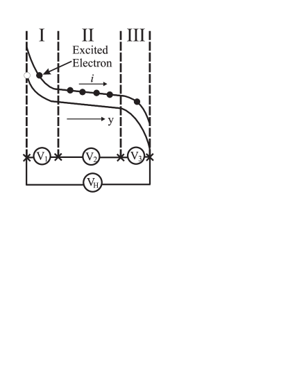
Figure 2: A schematic diagram showing the variation of the Landau level energy across the Hall bar. The e-h pairs are formed in region I by scattering from a charged impurity at a rate $W$. The cross-section of the bar is split into three regions. In regions I and III, near the edges of the bar, the voltage drop is high compared to region II in the centre of the hall bar.

Consider a local region of the sample where $E_{y}$ is large enough to create e-h pairs at a given rate, due to scattering from a charged impurity. A pair created close to an impurity drifts along the Hall bar at a velocity $E_{y}/B$, so for a fixed generation rate, a stream of e-h pairs moves along the Hall bar. Then, for a filling factor of 2 we have a situation in which a small fraction of electrons in the lower LL ($n=0$) have been replaced by holes and the previously empty upper LL ($n=1$) contains some electrons. As the e-h pairs move away from the high field region, the spacing between the electron and hole in a pair increases and most pairs eventually ionise by acoustic phonon emission. Due to the absence of empty states into which the excited electron can relax and neglecting weak, second order Auger processes, we can assume that all the generated e-h pairs eventually ionise, leading to a dissipative current $i=eW$, where $W$ is calculated from Eq. (1). This process is shown schematically in Fig. 2. From this figure we see that an e-h pair created close to the left (hot) edge of the Hall bar leaves a hole which ionises at the hot edge of the bar whilst the excited electron, in the $n+1$ Landau level, relaxes its energy due to phonon emission as it passes through regions I, II and III. At filling factor $\nu=2$, this process gives rise to a dissipative voltage

$$V_{x}=\left(\frac{hW}{2e}\right).$$ (3)

The NIST experiments carried out at $\nu=2$ and $B=12.3T$ show a series of up to 20 dissipative steps in $V_{x}$ of regular height $\Delta V_{x}\approx 5mV$. In Fig. 3 we plot our calculated dissipative voltage versus the background electric field $E_{y}$. Since $W$ is strongly influenced by the overlap between the wave-functions in the occupied ($n=0$) and unoccupied ($n=1$) LLs, it increases rapidly at a critical electric field. This occurs when $V_{x}$ is comparable to the small background dissipative voltage governed by $\sigma_{xx}$. The rate, W, and hence $V_{x}$, then reaches a maximum when the electric field is such that the e-h pairs are formed close to the roton minimum of the magneto-exciton dispersion curve. For a given $E_{y}$, for which $W$ is finite, the pairs formed at the breakdown point relax, so that electrons in the upper LL moving towards one side of the Hall bar, whilst holes move in the opposite direction. The presence of these carriers screens the Hall field over much of the Hall bar. Since the Hall voltage in the NIST experiments remains constant at its quantized value over the magnetic field range where the dissipative steps occur, this screening effect tends to enhance the electric field at the breakdown point. Thus, as the critical electric field is reached, the generation rate at the breakdown point increases rapidly, inducing a further increase in $E_{y}$ due to the screening of the Hall field in other regions of the Hall bar. We can see how this happens in Fig. 2. The electron is excited in region I and then decays due to phonon emission to region II. The voltage drop, $V_{2}$, is small so the electron takes a relatively long time to traverse this region. Hence, if the excited electrons in region I are generated at a constant rate, $W$, they tend to accumulate in region II. Since $V_{H}$ remains constant in the magnetic field range over which the steps are observed [2] and the accumulated electrons in region II screen the local electric field in this region the voltage drop, $V_{2}$, must reduce and hence the voltage dropped in regions I and III must increase. As a result, the electric field in regions I and III increases. This increase in $E_{y}$ increases $W$ until it reaches a maximum. Thus for breakdown at a single charged impurity the system should switch between two stable states, corresponding to $V_{x}=0$ and $V_{x}=5.6mV$, which corresponds to the maximum value of $V_{x}$ in Fig. 3. This is in good agreement with NIST experiments. In the experiments a series of up to twenty steps are observed and we attribute each step to the formation of separate streams of e-h pairs generated by different impurities.

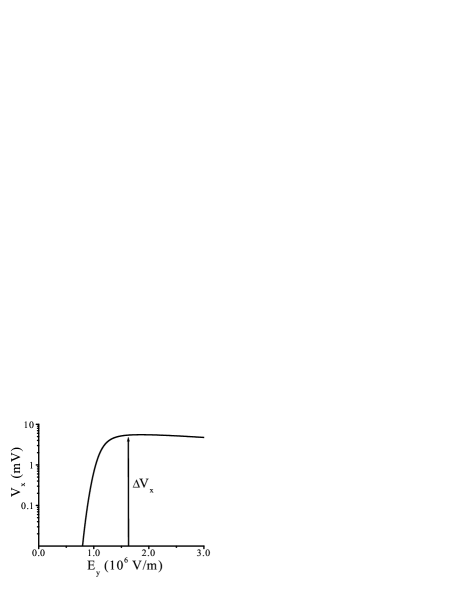
Figure 3: The dissipative voltage, for an electron gas sample, calculated from Eq. (3) as a function of $E_{y}$. The parameters used refer to the experimental conditions of [2].

We now examine more closely an analogy recently proposed by one of us [3] between the breakdown of the QHE and the breakdown of laminar fluid flow around an obstacle. Our starting point for such a model is an effective Euler equation, derived by Stone [7],

$$m^{\star}\left[{\bf\dot{v}}-\left[{\bf v}\times{\bf\Omega}\right]\right]=e\left({\bf E}+{\bf v}\times{\bf B}\right)-{\bf\bigtriangledown}\left(\frac{m^{\star}}{2}\left|{\bf v}\right|^{2}+\mu\right),$$ (4)

where ${\bf v}$ is the velocity field of the QHF, $\mu$ is the local chemical potential containing all the interaction terms and ${\bf\Omega}$ is the fluid vorticity. Examining small pertubations in the velocity and combining Eq. (4) with the continuity equation for the density of the QHF we find, in the limit ${\bf\bigtriangledown}\mu=0$,

$$\hbar\omega=\Delta\epsilon=-eE_{y}l_{B}(l_{B}Q)+\hbar\omega_{c}.$$ (5)

For $\Delta\epsilon=0$, this result is equivalent to Eq. (2) in the absence of interactions and corresponds exactly to the elastic inter-Landau level tunneling condition for the breakdown of the integer QHE [4]. Alternatively within this hydrodynamic model it corresponds to the condition required to generate a vortex-antivortex pairs at zero energy. From Eq. (5), we can deduce that for a fluid described by Eq. (4) laminar flow becomes unstable when

$$E_{y}=\frac{\hbar\omega_{c}}{el_{B}(l_{B}Q)}.$$ (6)

To make a direct comparison with our earlier quantum mechanical calculation we need to evaluate the dissipative voltage drop along the sample due to the generation of these vortex-antivortex pairs from a single impurity. For a specific system we would have to rely on a numerical simulation of Eq. (4). However, we can make considerable progress by considering vortex shedding in classical fluid mechanics [8]. Consider an obstacle in the path of a fluid. At a low fluid velocity the flow around the obstacle is laminar. When the flow rate is increased, vortex-antivortex pairs are formed in the vicinity of the obstacle. However, a vortex street is not formed until the flow is fast enough to free the vortex-antivortex pairs from the local flow field near the obstacle. In this steady state, each vortex-antivortex pair moves away from the obstacle at a velocity which is governed by the background fluid velocity. This analogy suggests that the vortex-antivortex pair in a QHF moves away from the impurity at a velocity given by $E_{y}/B$. From classical hydrodynamics [8] it is also known that the distance between each vortex-antivortex ($l$) pair generated is approximately three times the separation between a single vortex and antivortex ($d$) ($d/l=0.28$). Now consider two states for our fluid: firstly, the state where the fluid flow is laminar; then we know that the generation rate of vortex-antivortex pairs is zero. When $\Delta\epsilon=0$ it cost no energy to generate excitations and the flow ceases to become laminar due to the formation of vortex-antivortex pairs. Hence from Eq. (6) we can evaluate $E_{y}/B$. Dividing this velocity by the distance between each vortex-antivortex pair ($d=0.28l_{B}(l_{B}Q)$), to obtain the rate of generation of vortex-antivortex pairs, we obtain the voltage drop along the Hall bar as

$$V_{x}=\frac{0.28\pi\hbar\omega_{c}}{e(l_{B}Q)^{2}}.$$ (7)

To estimate the dissipative voltage step height from this hydrodynamic model we have to evaluate Eq. (7). We can do this by referring back to the previous quantum mechanical calculation to give us an estimate of $Ql_{B}$. Taking the value for $Ql_{B}=1.9$ for which the quantum calculations give the maximum value for $V_{x}$ we find, using Eq. (9) that $\Delta V_{x}=4.8mV$ for the NIST experiment [2].

In conclusion we have examined two models for the step-like breakdown of the integer QHE. The first is a full quantum calculation of the dissipative voltage drop along the Hall bar generated by scattering from a charged impurity. The second method uses an effective fluid model to describe the QHF from which we derive the elastic inter-Landau level tunneling condition [4]. From this condition and drawing analogies with classical fluid dynamics we also obtain $\Delta V_{x}$. In both cases we compared our theory to the experiments of Lavine et al. [2] which were carried out on the U.S. resistance standard sample. In each case the agreement between theory and experiment is quite good. It should also be noted that we have also made comparisons of our models with the step-like breakdown observed for a QHF of holes [9]; again our theoretical results match experiments quite well [10].

The models which we have presented above are for a specific type of breakdown in which $V_{x}$ increases as a series of steps of regular height. However, many samples do not exhibit such behaviour at breakdown. In such samples a single large increase in $V_{x}$ is observed at breakdown [5]. This behaviour is generally explained by the BSEH model [5], which describes an avalanche process which excites electrons over an extensive area of the sample. The model presented above does not contradict this model; in fact it complements it. Our model which describes a local breakdown due to scattering from charged impurities, can be a precurser to this avalanche breakdown which spreads over much of the sample, i.e. in some samples it is possible for the conditions for local charged impurity-induced breakdown to be met before the avalanche process takes over. The natural question then becomes what are these conditions and when can they be met. The condition for local charged impurity induced breakdown is sample specific; we require a locally high electric field in the region of a charged impurity to generate a stream of e-h pairs as compared to the total electric field across the sample reaching a critical value to trigger BSEH. We suggest that in the NIST samples some mechanism is inhibiting the avalanche, thus allowing us to observe the weaker local step-like breakdown.

This work is supported by the EPSRC.

References

- [1] M.E. Cage et al., Phys. Rev. Lett. 51, 1374 (1983).
- [2] C.F. Lavine, M.E. Cage and R.E. Elmquist, J. Res. Nat. Inst. Stand. Technol., 99, 757 (1994).
- [3] L. Eaves, Physica B 298, 1 (2001).
- [4] L. Eaves and F.W. Sheard, Semicond. Sci. Technol., 1, 346 (1986).
- [5] S. Komiyama et al., Solid State Commun. 54, 479 (1985); S. Komiyama et al., Phys. Rev. Lett. 77, 558 (1996); S. Komiyama, Y. Kawaguchi and T. Osada, Phys. Rev. B 61, 2014 (2000).
- [6] I.V. Lerner and Yu. E. Lozovik, Sov. Phys. JETP 51, 588 (1980); C. Kallin and B.I. Halperin, Phys. Rev. B 30, 5655 (1984); A.H. MacDonald, J. Phys. C 18, 1003 (1985).
- [7] M. Stone, Phys. Rev B 42, 212 (1990).
- [8] Mechanics of Fluids (sixth edition), B.S. Massey, Chapman and Hall (U.K.) (1989).
- [9] L. Eaves et al., Physica E 6, 136 (2000).
- [10] A.M. Martin et al., cond-mat/0201532 (unpublished).