Scale-Dependent Price Fluctuations for the Indian Stock Market

Abstract

Classic studies of the probability density of price fluctuations $g$ for stocks and foreign exchanges of several highly developed economies have been interpreted using a power-law probability density function $P(g)\sim g^{-(\alpha+1)}$ with exponent values $\alpha>2$, which are outside the Lévy-stable regime $0<\alpha<2$. To test the universality of this relationship for less highly developed economies, we analyze daily returns for the period Nov. 1994—June 2002 for the 49 largest stocks of the National Stock Exchange which has the highest volume of trade in India. We find that $P(g)$ decays as an exponential function $P(g)\sim\exp(-\beta g)$ with a characteristic decay scales $\beta=1.51\pm 0.05$ for the negative tail and $\beta=1.34\pm 0.04$ for the positive tail, which is significantly different from that observed for developed economies. Thus we conclude that the Indian stock market may belong to a universality class that differs from those of developed countries analyzed previously.

I Introduction

The market index is driven by numerous players and demand-supply factors through a composite average of various stocks. These factors constitute the complex market mechanism that causes the price variation in a component stock, which in turn pulls down or pushes up the a market index. Tracking many variables is tricky, making the quantification of economic fluctuations challenging.

A careful analysis of the market forces is required to provide accurate trends and indicators, which form a tool for market forecast and hence also provide solutions and key inputs for the improvement of economic policies and legislation. In this paper we investigate stock market asset price variations in a typical developing country such as India and compare the trends with those from economically developed economies.

A textbook study Hull of stock price variations suggests that stock prices—and concomitantly, stock price indices—follow a Markovian-Wiener process. This means that the stock price on any day is independent of the history of the stock price or its fluctuation. This results in a conventional log-normal density for stock prices Hull , i.e., the logarithm of the stock price follows a normal density.

However, developed markets such as those in the United States, Germany, and Japan exhibit a stock price behavior that differs from the Gaussian density frequently used in conventional theories. A key empirical finding in this regard is that the probability density of logarithmic price changes (returns) is approximately symmetric and decays with power law tails with identical exponent $\alpha\approx 3$ for both tails Lux ; Stocks . One intriguing aspect of this empirical finding is that it appears to be universal. Individual stocks appear to conform to these laws not just in US markets Stocks , but also in German Lux and Australian markets Allison . These same laws are obeyed by market indices such as the S&P 500, the Dow Jones, the NIKKEI, the Hang Seng, and the Milan index Index , and similar behavior is found in commodity markets Kaushik as well as in the most-traded currency exchange rates (e.g., the US dollar versus the Deutsch mark, or the US dollar versus the Japanese yen  Dacorogna ). The universal nature of these patterns exhibited in the statistics of daily returns is remarkable, since these markets differ greatly in their details. The observed universality is consistent with a scale-independent behavior of the underlying dynamics.

II Analysis

Here we focus on Indian stock market and find an exponential probability density function of price fluctuations, revealing an intrinsic scale. Our results is based on analyzing $\approx 10^{5}$ records representing daily returns for 49 largest stock of the National Stock Exchange (NSE) in India over the period Nov 1994—June 2002.

We define the normalized price fluctuation (return)

$$g_{i}(t)\equiv\frac{\log S_{i}(t+\Delta t)-\log S_{i}(t)}{\sigma_{i}}.$$ (1)

Here $\Delta t=1$ day, $i=1,2,..,49$ indexes the 49 stocks, $S_{i}(t)$ is the price of stock $i$ at time $t$, and $\sigma_{i}$ is the standard deviation of $\log S_{i}(t+\Delta t)-\log S_{i}(t)$.

To compare the probability density function of the Indian stocks with US stocks we randomly choose 49 US stocks in the same period. Next we aggregate the data note1 . Figures 1a and 1b displays the probability density function $P(g)$ for both positive and negative tails for the daily returns in a log-log plot. The US stocks have a power law probability density function with exponent $\alpha\approx 3$ [cf.  Lux ; Stocks ; Allison ; Index ].

Figures 1c and 1d displays the probability density of the aggregated data for both Indian and US stocks in a linear-log plot. We observe that the probability density of the 49 Indian stocks has an exponential form of decay

$$P(g)\sim e^{-\beta g}$$ (2)

with

$$\beta=\left\{\begin{array}[]{ll}1.51\pm 0.05&[\mathrm{negative~{}tail}]\\ 1.34\pm 0.04&[\mathrm{positive~{}tail}]\end{array}\right.$$ (3)

Figure 2 displays the estimates of $\beta_{i}$ for both positive and negative tails of the probability density function. We find the Kolmogorov-Smirnov (KS) significance probabilities for the null exponential hypothesis for all 49 Indian stocks and for the aggregated data to be $\ll 5\%$. Further we calculate

$$\beta_{\rm avg}\equiv\frac{1}{49}\sum_{i=1}^{49}\beta_{i}$$ (4)

and find

$$\beta_{\rm avg}=\left\{\begin{array}[]{ll}1.54\pm 0.05&[\mathrm{negative~{}tail}]\\ 1.34\pm 0.06&[\mathrm{positive~{}tail}]\end{array}\right.$$ (5)

III Discussion

Approximately $1/6$ of the world’s inhabitants live in India. In 2001 India had an estimated impoverished population of 40 million, 22% of the total urban population. The National Stock Exchange averages $6\times 10^{6}$ trades per day and its average daily turnover is $\approx 3\times 10^{8}$ USD. The average turnover in India is $\approx 10^{9}$ USD and the average share volume transacted is $\approx 2\times 10^{5}$. Because Indian people are traditionally extremely careful with their money, they have a high individual savings and transactions in the Indian Stock Market are not distributed across all economic scales. Stock market transactions are typically carried out by those with wealth in the top 25% of the economic spectrum.

A natural question is why the Indian stock market should have statistical properties that differ from other stock markets. One possible reason can be traced to the history of trading patterns in India and to its persistent trading culture. Even after more than 127 years of stock market operations, trading in India is said to be based as much on emotional factors as on actual evaluations and quantitative analysis.

Quantitative analytical skills, although available, are expensive and limited, so a majority of investors in India tend to follow archaic investment strategies, which they feel are more conservative and safe. The result is that extreme risk situations with concomitant high returns are completely avoided. This lack of quantification strategies has also hampered the two year old derivatives market, where even arbitrageurs trade on thumb rules and not actual models, we have witnessed prices where mis-pricing takes hours to correct. There are very few large financial institutions contributing to the total volume in trade. Small investors drive panic into the market on rumors making the market susceptible to small instabilities. Also, until recently, most Indian assets were under the control of the state and hence exposed to changes of political administration. These factors have kept the market under a tight noose.

Thus stock price fluctuations in India are intermediate to that between power law behavior and Gaussian behavior. Power law behavior is found for highly developed economies while the less highly developed economies such as India follow a behavior which is scale dependent. .

We thank L. A. N. Amaral, Y. Ashkenazy, X. Gabaix, P. Gopikrishnan, S. Havlin, V. Plerou, A. Schweiger and especially T. Lux for helpful discussions and suggestions, and NSF for financial support. M. P wishes to acknowledge C. Vasudevan, B. R. Prasad and Manoj Vaish for their kind encouragement and support.

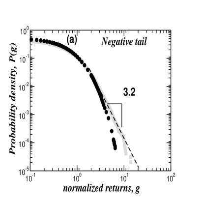
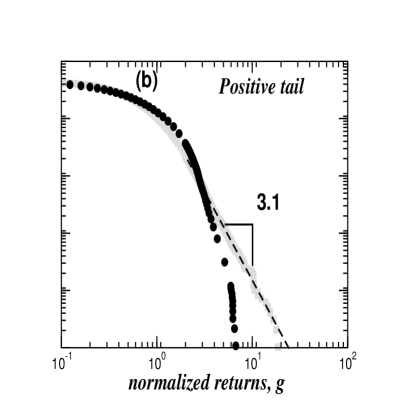
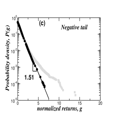
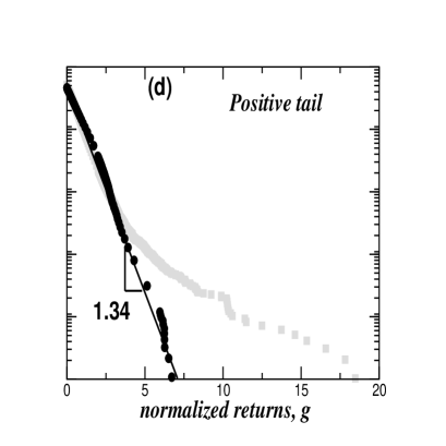
Figure 1: The probability density function of aggregated daily returns  note1 on a log-log plot for (a) the negative tail and (b) the positive tail. Solid symbols are aggregated data from 49 Indian stocks and the open squares are aggregated data from 49 US stocks over the same period, Nov. 1994—June 2002. The dashed lines are power law fits to the US data. The same data for aggregated daily returns on a linear-log plot for (c) the negative tail and (d) the positive tail. The solid lines have slopes $\beta=1.51\pm 0.05$ for the negative tail and $\beta=1.34\pm 0.04$ for the positive tail where the decay parameters and the error bars are estimated by the least square method. The KS significance probability of nullity of the exponential behavior hypothesis is $\approx 6.6\times 10^{-47}$.

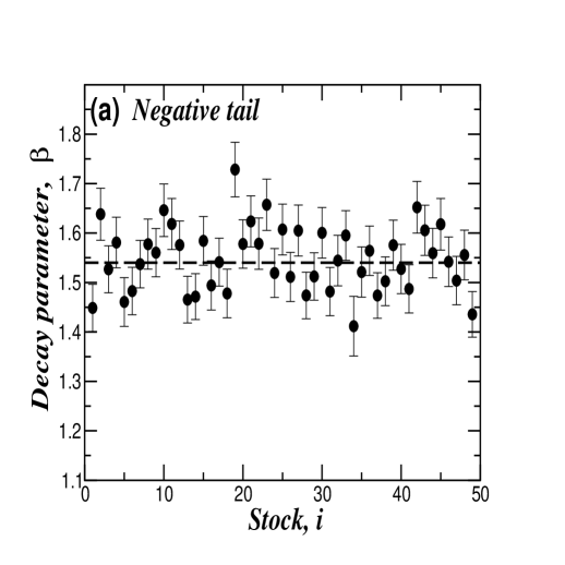
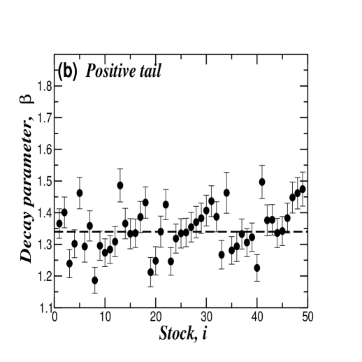
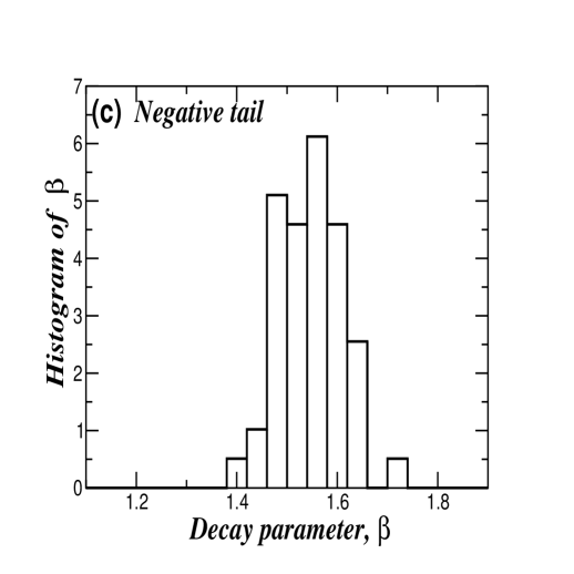
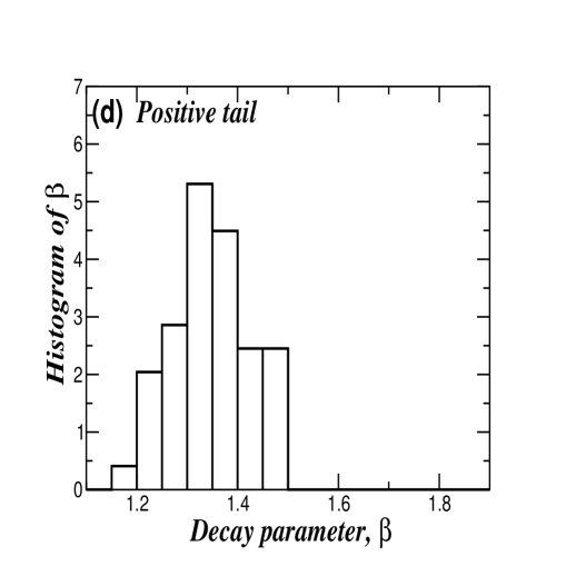
Figure 2: Decay parameters $\beta_{i}$ of (a) the negative tail and (b) the positive tail, where $i=1,2,..,49$ indexes the 49 Indian stocks analyzed. We employ a least square fit to estimate the parameters $\beta_{i}$ of each stock. The dashed lines show the average values defined in eqs. 4–5. Histogram of (c) the negative tail decay parameters $\beta_{\rm avg}=1.54\pm 0.05$, (d) the positive tail decay parameters$\beta_{\rm avg}=1.34\pm 0.05$ .

References

- (1) J. C. Hull Options, Futures and Other Derivatives (Prentice-Hall, Englewood Cliffs, New Jersey 2001).
- (2) T. Lux, Applied Financial Economics 6, 463 (1996).
- (3) P. Gopikrishnan, M. Meyer, L. A. N. Amaral, H. E. Stanley Eur. Phys. J. B 3, 139 (1998); Y. Liu, P. Gopikrishnan, P. Cizeau, M. Meyer, C. K. Peng, H. E. Stanley Phys. Rev. E 60, 1390 (1999); V. Plerou, P. Gopikrishnan, M. Meyer, L. A. N. Amaral, H. E. Stanley Phys. Rev. E 60, 6519 (1999).
- (4) A. Allison and D. Abbott, in Unsolved Problems of Noise, edited by D. Abbott and L. Kish (AIP Conf., Melville, New York, 2000).
- (5) R. N. Mantegna and H. E. Stanley, Nature 376, 46 (1995); P. Gopikrishnan, V. Plerou, M. Meyer, L. A. N. Amaral, H. E. Stanley Phys. Rev. E 60, 5305 (1999).
- (6) K. Matia, L. A. N. Amaral, S. Goodwin, and H. E. Stanley, Phys. Rev. E 66, 045103 (2002).
- (7) U A. Müller, M. M. Dacorogna, R. B. Olsen, O. V. Pictet, M. Schwarz, and C. Morgenegg, J. Banking and Finance 14, 1189 (1995); M. M. Dacorogna, U. A. Müller, R. J. Nagler, R. B. Olsen, and O. V. Pictet, J. Int’l Money and Finance 12, 413 (1993).
- (8) We aggregate the data, which is justified if the prices for all 49 stocks follow the same distribution. This assumption is consistent with our experience.