Phase diagram of 3D ANNNI model in an effective-field approximation

Abstract

An effective-field method for calculation of thermodynamic properties of three-dimensional lattice spin models is developed. It is applied to the ANNNI model on the simple cubic lattice. The phase diagram of the model, consisting of a large number commensurate phases and of an incommensurate phase, is calculated, confirming the results of previous approaches. The phase transition lines for a number of commensurate structures are localized and a strong evidence for absence of the direct phase transition between commensurate phases and the disordered phase is found.

I Introduction

In this paper we study the ANNNI model on a simple cubic or tetragonal lattice. This model was first introduced by Elliott ell in order to understand modulated magnetic materials. It is reviewed by Selke and Yeomans sel1 ; sel2 ; yeom . The model is known to form a low temperature ferromagnetic phase for a small next-nearest-neighbour interaction and a $\langle 2\rangle$ phase for a large one. The wedge in the nnn interaction-temperature phase diagram between this two phases is, at low temperatures, filled by infinite number commensurate phases.

Theoretical study of the ANNNI model has been based on a large number of various approaches. The devil’s staircase structure of the phase diagram at low and medium temperatures was elucidated by low-temperature series expansion fi1 and mean-field approximations boe ; bak1 ; fi2 ; sel3 ; jen . The incommensurate phase was also treated by the free fermion approximation vil ; ruj . Recently, an anisotropic scaling at the Lifshitz point was used to calculate several critical exponents at this point hen . A considerable effort was also devoted to investigation of ANNNI thin films sel4 ; sel5 ; sel6 .

The mean-field approximations describes qualitatively well the phase diagram of the ANNNI model, nevertheless, some of its features were challenged by other approaches, e.g. the stability of the commensurate phase up to the transition line to the disordered phase.

To improve the performance of mean-field treatment of the ANNNI model, we develop an effective field method, which is a generalization of the cluster transfer-matrix method successfully applied to 2D spatially modulated structures sur1 ; kar ; paj .

Our effective field method resembles the nonlinear mapping approach of Bak bak2 ; jen , but, instead of magnetization, it maps a large number of effective fields, which simulate the cluster environment. It is related also to the DMRG method sur2 , and for the 2D ANNNI model they yield similar results kar ; gen2 . Comparing with DMRG approach, our method is much simpler, and instead of diagonalization of density matrix and renormalization of transfer matrix by matrix multiplication it requires only calculation of square-root of a function of cluster spin configurations and real-number multiplications sur2 . The results of our method is in general agreement with other approaches, and it removes the artefacts of the previous mean-field methods.

In Section II the 3D ANNNI model is specified, and a new effective field approximation is developed. Results of numerical calculations and a tool for distingushing between commensurate and incommensurate phases, which lead to construction of the phase diagram are presented in Section III.

II Model and method

We shall generalize the cluster transfer-matrix method (an effective-field approximation) developed and applied to 2D space-modulated structures some time ago sur1 ; paj ; kar ; sur2 . The development of the 3D method follows the same ideas that were used in 2D case, however, a new approximation in the course of calculation has to be done. For reasons of clarity the method is developed for an ANNNI-type model but it can be easily reformulated for any 3D model with short-range interactions.

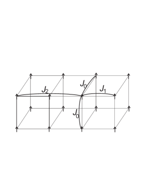
Figure 1: Spin-spin interactions in 3D ANNNI model; nn interactions $J_{0}$ and $J_{1}$ are ferromagnetic, nnn interactions $J_{2}$ are antiferromagnetic.

The three dimensional ANNNI model on a simple cubic lattice consists of two dimensional planes, within which each spin is coupled to its nearest neighbors by a ferromagnetic interaction $J_{0}$. However, in the direction perpendicular to the planes, spins are coupled by competing ferromagnetic nearest- and antiferromagnetic next-nearest-neighbor interactions (Fig. 1). For reasons of simplicity $J_{1}=J_{0}$ is further assumed.

As the interactions between spins $\sigma_{i,j,k}=\pm 1$ in the Hamiltonian of the 3D ANNNI model

$$H = \sum_{i,j,k}-J_{0}\sigma_{i,j,k}(\sigma_{i+1,j,k}+\sigma_{i,j+1,k})-J_{1}\sigma_{i,j,k}\sigma_{i,j,k+1}$$ (1)

$$+J_{2}\sigma_{i,j,k}\sigma_{i,j,k+2}$$

involve only three layers, it can be written as a sum of layer Hamiltonians $H_{i}(S_{i},S_{i+1},S_{i+2})$ which depend on three layer variables $S_{k}\equiv\{\sigma_{i,j,k}\}\ i,j\in(-\infty,\infty)$. Since there are only nearest-neighbor interactions inside the layers, the layer Hamiltonian can be expressed as a sum of cluster Hamiltonians defined on $2\times 2\times 3$ clusters with the longer side oriented along the $J_{2}$ interaction.

$$H=\sum_{k}(H_{k}(S_{k},S_{k+1},S_{k+2})=\sum_{k}\sum_{i,j}H_{i,j,k}(\sigma_{l,m,n})$$ (2)

where $l=i,i+1,\ m=j,j+1,\ n=k,k+1,k+2$.

The exponential of the layer Hamiltonian $H_{k}$ is further denoted by $T_{k}(S_{k},S_{k+1},S_{k+2})\equiv\exp[\beta H_{k}(S_{k},S_{k+1},S_{k+2})]$ and sometimes called transfer matrix though it is rather a function of spin variables.

Then the summation in the partition function

$$Z=\sum_{\{\sigma_{i}\}}\exp[\beta H(\sigma_{i})]$$

may be performed consecutively layer by layer generating a set of auxiliary functions $\Psi_{k}$ and normalization factors $\lambda_{k}$

$$\sum_{S_{k}}\Psi_{k}(S_{k},S_{k+1})T_{k}(S_{k},S_{k+1},S_{k+2})=\lambda_{k}\Psi_{k+1}(S_{k+1},S_{k+2})$$ (3)

starting from an appropriate function $\Psi_{1}(S_{1},S_{2})$ that may be interpreted as a boundary condition of the system on a semi-infinite lattice. The values of $\Psi_{k}$ for $k\to\infty$ mostly do not depend on the input $\Psi_{1}$ except the vicinity of a first order phase transition. Here the different bulk values correspond to one stable and one or more physically unstable solutions. The stable solution is the one with the lowest free energy that is proportional to $\log\prod_{k}\lambda_{k}$.

As we see, the auxiliary functions in the transfer matrix method are some general positive functions defined on clusters of planes in 3D models. For lower-dimensional models they are defined on clusters of rows in 2D and clusters of sites in 1D. In a one-dimensional model, the auxiliary functions depend on finite number of spin variables, in 2D and 3D cases they acquire infinite number of values which cannot be generally found by numerical calculations. Instead of the whole function at the right-hand side of (3), we further calculate only its correlation function, sum of $\Psi_{k+1}(S_{k+1},S_{k+2})$ over the whole lattice except a small cluster, and the true auxiliary function $\Psi$ is approximated by a more convenient one, nevertheless, exactly reproducing the calculated correlation functions.

As we do not use any further information from the left-hand side of Eq. (3), all the remaining properties of the approximate function $\tilde{\Psi}$ are derived from the requirement of maximum of the information entropy $S=\tilde{\Psi}\log\tilde{\Psi}$ jaynes . To maximize $S$ under the condition that the partial sum of $\tilde{\Psi}$ is equal to the given correlation function, Lagrange multipliers corresponding to each configuration of the cluster have to be introduced. It is easy to show that the desired auxiliary function can be expressed as a product of exponentials of the cluster Lagrange multipliers. Thus, the requirement of maximum of the information entropy leads to a factorization of the auxiliary function. If only factorized auxiliary functions are used, the left-hand side of (3) is completely factorized for short-range interactions and its partial summation is equivalent to calculation of a correlation function of a statistical system of the dimension lower by 1 than that of the original problem. It means that for 2D system this step can be performed exactly, but for 3D the factorization procedure must be applied even for calculation of the correlation function.

In the case of 2D model (1D auxiliary functions) the application of the above considerations is straightforward. Let us denote the correlation function on a small cluster of the length $n+1$ by

$$\Phi_{i}^{i+n}\equiv\hskip-15.0pt\sum_{\{\sigma_{j}\}\atop j\in(-\infty,i)(i+n,\infty)}\hskip-15.0pt\Psi(\sigma_{j}),$$

which is assumingly known from the previous calculation step. The approximate function $\tilde{\Psi}$ is defined as a product of unknown cluster functions $\Theta_{i}^{i+n}(\sigma_{j})$ defined on $n+1$ sites:

$$\tilde{\Psi}\equiv\prod_{i}\Theta_{i}^{i+n}(\sigma_{j})\qquad j\in\langle i,i+n\rangle.$$ (4)

We would like to express the cluster functions $\Theta_{i}^{i+n}$ in terms of $\Phi_{i}^{i+n}$.

Let us denote the left eigenfunction of the function (transfer matrix) $\Theta_{i}^{i+n}$

$$\sum_{\sigma_{i}}\theta_{i}^{i+n-1}(\sigma_{j})\Theta_{i}^{i+n}(\sigma_{j})=\lambda\theta_{i+1}^{i+n}(\sigma_{j})$$ (5)

by $\theta$ and its eigenvalue by $\lambda$. ($\theta_{i}^{i+n-1}$ and $\theta_{i+1}^{i+n}$ are identical function defined on different clusters if we do not expect any space modulation in this direction.)

Since $\theta_{i}^{i+n-1}$ is the result of summation of $\tilde{\Psi}$ from $-\infty$ to $i$, correlation function $\tilde{\Phi}_{i}^{i+n}$ corresponding to $\tilde{\Psi}$ can be expressed as

$$\tilde{\Phi}_{i}^{i+n}=\theta_{i}^{i+n-1}\Theta_{i}^{i+n}\bar{\theta}_{i+n}^{i+1},$$

where $\bar{\theta}$ is the right eigenfunction of $\Theta$ defined by

$$\sum_{\sigma_{i+n}}\Theta_{i}^{i+n}(\sigma_{j})\bar{\theta}_{i+n}^{i+1}(\sigma_{j})=\lambda\bar{\theta}_{i+n-1}^{i}(\sigma_{j}).$$ (6)

Since we require $\tilde{\Phi}_{i}^{i+n}=\Phi_{i}^{i+n}$, the unknown cluster function $\Theta^{i+n}_{i}$ is

$$\Theta_{i}^{i+n}={\Phi_{i}^{i+n}\over\theta_{i}^{i+n-1}\bar{\theta}^{i+1}_{i+n}}.$$ (7)

Unfortunately, the eigenfunctions $\theta$ and $\bar{\theta}$ are implicit functions of $\Theta$. On the other hand, it can be easily shown that

$$\Theta_{i}^{\prime\,i+n}=\sqrt{\theta_{i}^{i+n-1}\over\bar{\theta}^{i}_{i+n-1}}\,\Theta_{i}^{i+n}\,\sqrt{\bar{\theta}_{i+n}^{i+1}\over\theta^{i+n}_{i+1}}$$ (8)

have the same eigenvalues as the original cluster functions $\Theta_{i}^{i+n}$. Substituting (7) for $\Theta_{i}^{i+n}$ we get

$$\Theta_{i}^{\prime\,i+n}={\Phi_{i}^{i+n}\over\sqrt{\theta_{i}^{i+n-1}\bar{\theta}_{i+n-1}^{i}\theta_{i+1}^{i+n}\bar{\theta}_{i+n}^{i+1}}}={\Phi_{i}^{i+n}\over\sqrt{\Phi_{i}^{i+n-1}\Phi_{i+1}^{i+n}}},$$ (9)

where $\Phi_{i+1}^{i+n}=\sum_{\sigma_{i}}\Phi_{i}^{i+n}=\theta_{i+1}^{i+n}\bar{\theta}_{i+n}^{i+1}$ and similarly $\Phi_{i}^{i+n-1}$. Thus, obeying the condition of maximum of information entropy, relations (4, 9) yield a possibility to express the approximate chain auxiliary function $\tilde{\Psi}$ in terms of the known correlation function $\Phi_{i}^{i+n}$

$$\Psi\approx\tilde{\Psi}=\prod_{i}\Theta_{i}^{i+n}=\prod_{i}\Theta_{i}^{\prime\,i+n}=\prod_{i}{\Phi_{i}^{i+n}\over\sqrt{\Phi_{i}^{i+n-1}\Phi_{i+1}^{i+n}}}$$ (10)

In the case of 2D auxiliary function (for 3D models) the relation (10) is further valid, only the indices denote infinite rows of sites rather than sites. However now, we cannot expect that the correlation function $\Phi_{i}^{i+n}$ defined on $n+1$ infinite rows could be found in previous calculations, but only a function on a finite cluster of the size $n\times l$. We denote it by $\Phi_{i,j}^{i+n,j+l}$, where the first indices represent rows and the second ones columns of the lattice. The most serious difference between 3D and 2D models is that the eigenfunction in (5) cannot be found exactly but it must be factorized, as well. Then all the functions in the expression for $\Phi_{i}^{i+n}$ are factorized similarly as at the left-hand side of Eq. (3), i.e. the whole procedure that we applied to the chain auxiliary function $\Psi$, and that has led to (9), can be applied to $n$-row and $n-1$-row correlation function $\Phi_{i}^{i+n}$ and $\Phi_{i+1}^{i+n}$, $\Phi_{i}^{i+n-1}$, respectively, appearing in 2D version of (10). We obtain

$$\Phi_{i}^{i+n}=\prod_{j}{\Phi_{i,j}^{i+n,j+l}\over\sqrt{\Phi_{i,j}^{i+n,j+l-1}\Phi_{i,j+1}^{i+n,j+l}}}\qquad\hbox{etc.}$$ (11)

Thus, by consecutive application of the factorizing procedure (11) to all terms in (10), an approximation $\tilde{\Psi}$ to the function $\Psi$ can be expressed in terms of its cluster correlation function

$$\Phi_{i,j}^{i+n,j+l}=\hskip-15.0pt\sum_{{\{\sigma_{km}\}\atop k\in(-\infty,i)\cup(i+n,\infty)}\atop m\in(-\infty,j)\cup(j+l,\infty)}\hskip-15.0pt\Psi(\sigma_{km}).$$ (12)

The expression reads

$$\Psi\approx\tilde{\Psi}=\prod_{i,j}\Theta_{i,j}^{\prime i+n,j+l}\hfill$$ (13)

$$=\prod_{i,j}{\Phi_{i,j}^{i+n,j+l}\root 4 \of{\Phi_{i,j}^{i+n-1,j+l-1}\Phi_{i,j+1}^{i+n-1,j+l}\Phi_{i+1,j}^{i+n,j+l-1}\Phi_{i+1,j+1}^{i+n,j+l}}\over\sqrt{\Phi_{i,j}^{i+n,j+l-1}\Phi_{i,j+1}^{i+n,j+l}\Phi_{i,j}^{i+n-1,j+l}\Phi_{i+1,j}^{i+n,j+l}}}$$

Unlike in 1D case, the correlation function calculated from $\tilde{\Psi}$ is only approximately equal to that calculated from $\Psi$. It would be true if we were able to factorize the whole two-dimensional plane function $\Theta^{\prime i+n}_{i}$ in 2D version of (10) and not only each correlation function $\Phi$ separately.

All the functions in (13) are plane dependent in the case of a modulated structure. Therefore, in the explicit description of the iteration procedure, the plane index $k$ should be attached to all correlation and auxiliary function.

The logarithm of the cluster functions $\Theta^{\prime}$ may be interpreted as effective fields acting on a plane, simulating the effect of the half-lattice already summed up. However, for simplicity, the functions $\Theta^{\prime}$ themselves will be called effective fields.

The computational iteration scheme of the cluster transfer-matrix method for 3D ANNNI model is as follows:

1. From the cluster functions (effective field) ${}_{k}\Theta_{i,j}^{\prime i+n,j+l}$ known from the previous step the approximate auxiliary function $\tilde{\Psi}_{k}(S_{k},S_{k+1})=\prod_{i,j}\,{}_{k}\Theta_{i,j}^{\prime i+n,j+l}$ is constructed and $\Psi_{k}(S_{k},S_{k+1})$ in (3) is replaced by it.

2. The correlation function ${}_{k+1}\Phi_{i,j}^{i+n,j+l}$ (12) of the auxiliary function $\Psi_{k+1}(S_{k+1},S_{k+2})$ is calculated from (3). As the both functions at the left-hand side of (3) are factorized this problem is equivalent to calculation of a correlation function of a 2D lattice model with short-range interactions that was discussed above and in previous papers sur1 ; kar ; paj in detail. This task is performed in two steps, and the approximate factorization utilizing 1D version of (10) is applied once.

3. Formula (13) is used and the cluster functions ${}_{k+1}\Theta_{i,j}^{\prime i+n,j+l}$ are found.

4. Calculation is continued for the next plane starting from the step 1.

It is convenient to take the result of a previous iteration for the initial condition of the calculation at a nearby point in the parameter space. The bulk values of the cluster function are obtained after iteration over few periods of the commensurate or incommensurate structure. However, the periods of the commensurate structure sometimes exceed several hundreds of lattice constants in our calculations. The convergence of the iteration procedure is very slow near the continuous incommensurate-disorder phase transition and the steady state were reached after more than ten thousands steps.

In our actual calculations the length of the cluster edges $n$ and $l$ was taken equal to 1, i.e. the cluster on which the functions $\Phi_{i,j}^{i+n,j+l}$ and $\Theta_{i,j}^{\prime i+n,j+l}$ are defined has 8 sites (elementary cube) and the functions acquire 256 values. Thus, our generalized mean-field approximation utilizes 256 effective fields instead of one in previous approaches. jen

The planes perpendicular to the nnn interaction are ferromagnetic in the ANNNI model, thus the cluster correlation function and the cluster function do not depend on its position in the plane. ${}_{k}\Phi_{i,j}^{i+n,j+l}$ is in fact only a short-hand notation of $\Phi_{k}({}_{k}S_{i,j}^{i+n,j+l})$, where ${}_{k}S_{i,j}^{i+n,j+l}$ is a spin configuration of a cluster in the plane $k$. Similarly, ${}_{k}\Theta_{i,j}^{\prime i+n,j+l}\equiv\Theta_{k}^{\prime}({}_{k}S_{i,j}^{i+n,j+l})$.

To find the actual structure at the given point of the phase diagram, it is not necessary to calculate the lattice site magnetizations. The structure can be deduced from the plane dependence of the effective field $\Theta_{k}^{\prime}$. In our approximation it acquires 256 values, but a plot of arbitrary one of them can be used to find the phase diagram. For reason of simplicity and symmetry, the difference $\psi_{k}\equiv\Theta_{k}^{\prime}(+)-\Theta_{k}^{\prime}(-)$, is plotted where “+” and “$-$”denote spin configurations of the 8-site cluster with all the spins up and down, respectively. The sign of the function $\psi_{k}$ is the same as the sign of the magnetization of the $k$-th row. The ANNNI model structures consist of sequences of planes with negative or positive magnetization. As the external magnetic field is equal to zero, the commensurate structures are symmetric with respect to spin inversion. Therefore, only $|\psi_{k}|$ is taken into account further. Its periodicity $p$ is one half of or equal to the structure periodicity if in the interval $p$ the function $\psi_{k}$ changes its sign even or odd times, respectively. A structure consisting repeatedly of $p$ planes with positive magnetization and $p$ planes of negative magnetization with periodicity $2p$ is usually denoted in literature as $\langle p\rangle$. More generally, the sequence of $n$ clusters of the above-mentioned planes of the length $p$ interrupted by one cluster of the length $p-1$ is denoted as $\langle p^{n}(p-1)\rangle$.

At high temperature when the convergence is slow and the areas of commensurate structures are very narrow, or at lower temperatures when near the accumulation points the periodicity of commensurate structures tends to infinity, it is often not possible to perform the calculation directly at the point of parameter space of desired properties, because its precise position is not known. Nevertheless, the structure at it can be deduced from the behavior of the effective field in its close vicinity. For this purpose, we shall further plot $|\psi_{k+p}|-|\psi_{k}|$ vs. $|\psi_{k}|$, where $p$ is the periodicity of the function $|\psi_{k}|$ somewhere near the point of the parameter space where we perform the calculation. It is not necessary to plot $|\psi_{k+p}|-|\psi_{k}|$ vs. $|\psi_{k}|$ for all values of $k$. The information, we are interested in, can be found from behavior of the plot for the planes $k_{0}+np$ $(n=1,2,\dots)$. $k_{0}$ should be the number of the plane closest to a node of the structure $({\rm sign}\,\psi_{k_{0}}\neq{\rm sign}\,\psi_{k_{0}+1})$, where $|\psi_{k_{0}}|$ is close to zero and $|\psi_{k_{0}}|-|\psi_{k_{0}-1}|$ is large. Now, $|\psi_{k+p}|-|\psi_{k}|=0$ always means that the structure is commensurate with period $p$ or $2p$ and not that $|\psi_{k}|$ is close to its maximum value. The plots will be drawn for $|\psi_{k}|$ in the range from 0 to its maximum value when a new plane $k-1$ with a smaller value of $|\psi_{k-1}|$ appears. Analysis of them will make possible to distinguish between commensurate and incommensurate structures and confirm the existence of the accumulation point, where period of commensurate structures tends to infinity.

III Results and discussion

Results of our effective-field calculations are consistent with the phase diagram obtained by the mean-field approximation and low-temperature expansion [sel1]. However, the temperatures, at which the phase transitions occur, are more realistic, and for the exactly soluble case $J_{2}=0$ the critical temperature does not deviate more than 1% from the true value for the approximation with 256 effective fields.

From our calculation, in accordance with previous results of other authors, it is possible to conclude that the phase diagram consists of infinitely many commensurate phases which appear mostly at low temperatures and an incommensurate and disordered phase at high temperatures.

At low temperature we have found a ferromagnetic phase, a commensurate structure with periodicity 4 consisting of a sequence of couples of planes with alternating magnetization ($\langle 2\rangle$), a structure with periodicity 6 ($\langle 3\rangle$) and combinations of the last two structures of the type $\langle 2^{n}3\rangle$ $n=1,2,3,\dots$. As the low-temperature region is fairly well described by the low-temperature expansion, we concentrate to the medium- and high-temperature properties of the phases $\langle 4\rangle$, $\langle 3\rangle$, $\langle 23\rangle$ and the regions in their close vicinity.

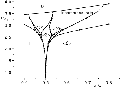
Figure 2: Phase diagram of the 3D ANNNI model. Only the basic structures with short periodicity are depicted. The dotted lines connect points in the parameter space where the incommensurate phase has the same periodicity as the corresponding commensurate structure. The symbols denote the following periodically repeating structures: $\langle 2\rangle$ – $\uparrow\uparrow\downarrow\downarrow$, $\langle 3\rangle$ – $\uparrow\uparrow\uparrow\downarrow\downarrow\downarrow$, $\langle 23\rangle$ – $\uparrow\uparrow\downarrow\downarrow\downarrow$, $\langle 4\rangle$ – $\uparrow\uparrow\uparrow\uparrow\downarrow\downarrow\downarrow\downarrow$, F – ferromagnetic $(\uparrow)$, D – disordered, where the arrows indicate directions of plane magnetization.

The main phases of the 3D ANNNI model obtained from our calculations are shown in the phase diagram (Fig. 2). The thick lines denote the borders of the regions of commensurate phases and represent first-order phase transition lines. The dotted lines connect points in the parameter space where the incommensurate phase has the same periodicity as the corresponding commensurate structure. The widths of the commensurate phases near the order-disorder phase transition line go to zero for all of them, i.e., there is no direct transition between the commensurate and the disordered phase. The commensurate regions at high temperatures are very narrow (narrower than the line thickness), nevertheless, they persist to rather high temperatures. A very large (probably infinite) number of commensurate phases between each two main phases are not depicted in the diagram and are discussed later. The Lifshitz point behind the left edge of the diagram is not shown, as the slow convergence of calculations and complicated phase structure did not make possible to correctly interpret the obtained results.

It is not easy to prove the existence of the commensurate phase in a very narrow region and distinguish between the commensurate and incommensurate phase of the same or a slightly different periodicity. Here, it is helpful to observe the above-mentioned plot of $\Delta\psi\equiv|\psi_{k+p}|-|\psi_{k}|$ vs. $|\psi_{k}|$, where $p$ is the periodicity of the function $|\psi_{k}|$ for the assumed commensurate structure.

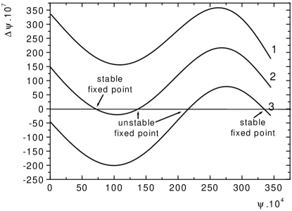
Figure 3: Plot of $\Delta\psi\equiv|\psi_{k+3}|-|\psi_{k}|$ vs. $\psi\equiv|\psi_{k}|$ for every third plane of $\langle 3\rangle$ structure. $T=3.45$. The plots are drawn for the following values of the parameters: 1 – $J_{2}/J_{1}=0.53335$, 2 – $J_{2}/J_{1}=0.53325$, 3– $J_{2}/J_{1}=0.53315$. The commensurate $\langle 3\rangle$ phase is represented by the stable fixed point. Curve 1 represents an incommensurate structure. As $\Delta\psi\ll\psi$, the plots are practically continuous.

In Fig. 3 this plot for $T=3.45$ and two different $J_{2}/J_{1}$ inside and near the structure $\langle 3\rangle$ is shown. $p=3$, and $k$ runs over all planes after which $\psi_{k}$ changes its sign, i.e. we plot the function for every third plane. The structure is commensurate if $\Delta\psi$ is equal to zero. We see that for $J_{2}/J_{1}=0.53335$ it never occurs. The function is incommensurate one with local periodicity greater than 3, and it changes at different places of the structure, i.e. the true periodicity is very large, and for decreasing $J_{2}/J_{1}$ it tends to infinity. It can be considered as a phase-modulated $\langle 3\rangle$ structure. As the curve $|\psi_{k+p}|-|\psi_{k}|$ vs. $|\psi_{k}|$ shifts in vertical direction with change of $J_{2}/J_{1}$ with only a small change of its shape, we can expect that for some values of $J_{2}/J_{1}$ the curve intersects the $x$-axis and the structure becomes commensurate. In Fig. 3 this situation is exemplified by the curves for $J_{2}/J_{1}=0.53325$ and 0.53315. In the bulk the structure is $\langle 3\rangle$, the difference $|\psi_{k+p}|-|\psi_{k}|$ is equal to zero and the structure is trapped in the stable fixed point. In the transition period, near the surface or a planar defect, where $\Delta\psi\neq 0$, the structure is incommensurate-like. Starting away from an arbitrary boundary condition the system reaches very fast an incommensurate metastable state, represented by one of the curves, from which the stable bulk commensurate structure at the intersection with $x$-axis slowly develops.

To confirm the existence of the commensurate structure in some region of parameter space, it is not necessary to find the point where after many iteration steps the system converges to a bulk commensurate structure. Near to it $\Delta\psi$ is small and the convergence is very slow. It is enough to find a nonmonotonous behaviour of the $\Delta\psi$ vs. $\psi$ plot of an incommensurate structure somewhere near that parameter space point. A set of such plots for $T=3.52$ is shown in Fig. 4. It is seen that the amplitude of modulation of the functions increases when approaching the commensurate phase. Thus, already a small modulation of the curve far from the commensurate structure indicates its presence.

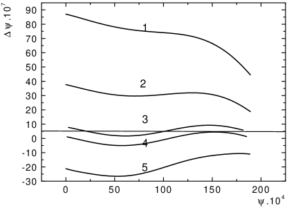
Figure 4: Plot of $\Delta\psi\equiv|\psi_{k+3}|-|\psi_{k}|$ vs. $\psi\equiv|\psi_{k}|$ for every third plane and high-temperature, $T=3.52$, $\langle 3\rangle$ structure. The plots are drawn for the following values of the parameters: 1 – $J_{2}/J_{1}=0.534400$, 2 – $J_{2}/J_{1}=0.534350$, 3 – $J_{2}/J_{1}=0.534320$, 4 – $J_{2}/J_{1}=0.534313$, 5 – $J_{2}/J_{1}=0.534290$. The commensurate $\langle 3\rangle$ phase is represented by curve 4.

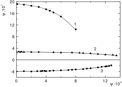
Figure 5: In close vicinity of the phase transition line to the disordered state all the plots $\Delta\psi\equiv|\psi_{k+3}|-|\psi_{k}|$ vs. $\psi\equiv|\psi_{k}|$ are monotonous indicating the absence of commensurate phase in this region. 1 – $T=3.5461,\ J_{2}/J_{1}=0.5341$; 2 – $T=3.5465,\ J_{2}/J_{1}=0.5345$; 3 – $T=3.5466,\ J_{2}/J_{1}=0.5346$.

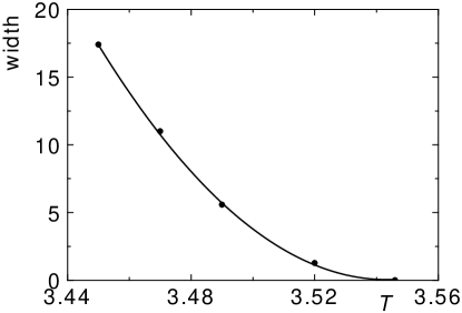
Figure 6: Plot of the width of the commensurate phase $\langle 3\rangle$ vs. temperature. The width is given in the units of $J_{2}/J_{1}\cdot 10^{-4}$.

The width of the region of the commensurate structure can be deduced from the amplitude of the function $|\psi_{k+p}|-|\psi_{k}|$ vs. $|\psi_{k}|$ and the rate of its vertical shift with change of the parameters.

Fig. 5 shows that for $T=3.546$ no commensurate $\langle 3\rangle$ structure exists. All the curves are monotonous. The sign of their derivatives is negative and positive above and below the $x$-axis, respectively, and they do not intersect it. The period of $\psi$ close to 3. The point in the parameter space is now very close to the order-disorder phase transition line, so that the parameters in Fig. 5 should be carefully changed only in the direction parallel to it. The rate of convergence is very slow here, and the bulk incommensurate structures depicted in the figure were obtained after more than 10,000 iteration steps. The argument of nonexistence of commensurate structure at $T=3.546$ is confirmed by extrapolation of the widths of the $\langle 3\rangle$ structure to higher temperatures shown in Fig. 6. For small values of the width, this plot could be well fitted by a parabola.

Similar considerations were done for the structures $\langle 4\rangle$, $\langle 23\rangle$ and $\langle 23^{20}\rangle$ and it was found that the commensurate structures of higher periodicity disappear at lower temperatures. The whole region near the order-disorder phase transition line is incommensurate with tongues of commensurate structures of low periodicity which do not reach the phase transition line.

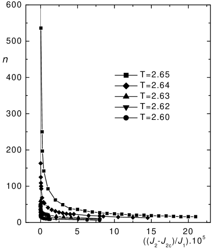
Figure 7: Number $n$ of $\uparrow\uparrow\uparrow$ or $\downarrow\downarrow\downarrow$ plane sequences in $\langle 23^{n}\rangle$ commensurate phases near the transition line to $\langle 3\rangle$ structure. The value of $J_{\rm 2c}$ at the transition line is different for each temperature. $n$ acquires discrete values and the lines are only guides for the eye.

At very low temperatures the phase $\langle 3\rangle$ is neighboring to the phase $\langle 23\rangle$. With increasing temperature, at $T=1.6$, phases of the type $\langle 23^{n}\rangle$ start to appear. At given temperature $T$ the period of the structure, $p=3n+2$, increases with decreasing $J_{2}/J_{1}$ and its largest value is reached at the boundary of the $\langle 3\rangle$ structure. The plots of $n$ near the $\langle 3\rangle$ boundary for $T=2.60,2.62,2.63,2.64,2.65$ are depicted in Fig. 7. The periodicity in the close vicinity of $\langle 3\rangle$ phase increases very fast and for the temperatures above 2.62 it is not possible to determine the value of $n_{\rm max}$ or even decide if it is finite or not. Nevertheless, the accumulation point, where $n_{\rm max}$ becomes infinite, can be found analyzing the plots $|\psi_{k+p}|-|\psi_{k}|$ vs. $|\psi_{k}|$ for different temperatures and $p=3$, which are shown in Fig. 8. The structure $\langle 23^{n}\rangle$ for large $n$ is formed from domains of the structure $\langle 3\rangle$ of the length slightly less than $n$ interrupted by domain walls symbolically denoted by “2” in the symbol $\langle 23^{n}\rangle$. The $\langle 3\rangle$ structure beyond the wall is shifted by one plane with respect to the structure in the previous domain. The $\langle 3\rangle$ domains correspond to the minima of the plots in Fig. 8 where the $|\psi_{k+3}|-|\psi_{k}|$ are practically equal to zero. The advent of the wall is so abrupt and $|\psi_{k+3}|-|\psi_{k}|$ so large that the next point after the very right edge of the each curve is already out of scope of the diagram. With decreasing $J_{2}/J_{1}$ the plots are shifting down and at the $\langle 3\rangle$ phase transition line the minimum of the plot touches $x$-axis, and after some transition period the system remains stuck in $\langle 3\rangle$ phase. If the slope of the plot at minimum is zero, the periodicity near the boundary tends to infinity, and the temperature of the system is already above the accumulation point. From Fig. 8 we see that the accumulation point is close to the temperature $T=2.64$. The periodicity of $|\psi|$ tends to infinity if the curve approaches $x$-axis for $J_{2}\rightarrow J_{\rm 2c}$ at $T=2.65$. Using our method, we were able to find a commensurate structure of $p=1802$ at this temperature.

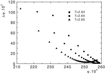
Figure 8: Plot of $\Delta\psi\equiv|\psi_{k+3}|-|\psi_{k}|$ vs. $\psi\equiv|\psi_{k}|$ for commensurate $\langle 23^{n}\rangle$ structures near transition to $\langle 3\rangle$ phase. $n$ is equal to the number of points along each curve. (Only points for small value of $\Delta\psi$ are depicted in the figure.) The curves for $J_{2}=J_{2c}$ touch the $x$-axis. For curves with zero derivative in the minimum $n$ tends to infinity.

For temperatures lower than the temperature of accumulation point near the boundary of the $\langle 3\rangle$ phase only plain $\langle 23^{n}\rangle$ phases exist. This is in contradiction with the simple mean field approximation findings sel1 . There is also a difference in location of the accumulation point. In sel3 it was found well below the turning point of the $\langle 3\rangle$ boundary where the width of the $\langle 3\rangle$ phase starts becoming narrower. Our approach locates the accumulation point $T=2.64$ slightly above the turning point. Approximately at the same temperature first combined phases of the type $\langle(23^{n})(23^{n+1}))\rangle$ between $\langle(23^{n})\rangle$ and $\langle(23^{n+1}))\rangle$ for large $n$ start to appear. Similarly to the previous more simple case, following combinations in the hierarchy are of the type $\langle((23^{n}))^{k}(23^{n+1}))\rangle$ or $\langle(23^{n})((23^{n+1}))^{k})\rangle$, which appear at temperatures by 0.04 higher than the temperature of the accumulation point. A great computational effort is needed to detect a next type of combinations $(\langle((23^{n}))^{k}(23^{n+1})))^{l}(\langle((23^{n}))^{k+1}(23^{n+1})))\rangle$. These high-order combinations occupy very small areas of the parameter space, and with increasing temperature they are soon replaced by incommensurate structures.

It is widely believed that the structures with large distances between the domain walls are commensurate whereas the structures where the distance between the walls is shorter than the wall-wall interaction are incommensurate. This statement should be formulated more precisely. The commensurate structures with short distances between the walls are more stable than those with longer distances. They persist to higher temperatures and they occupy a wider area in the parameter space. Nevertheless, in the areas between $\langle(23^{n})\rangle$ and $\langle(23^{n+1}))\rangle$ for small $n$ the onset of incommensurate structures was found at lower temperatures than for large $n$. The distance between the commensurate structures increases with decreasing $n$ faster than their width so that there is enough space for incommensurate structures.

In summary, we developed an effective field approximation, wihich yields by simple iteration procedure practically any of probably an infinite number of phases in the phase diagram of the 3D ANNNI model. In fact, the method treats an infinite lattice. Lattice size, in contrast to other mean-field and DMRG approaches, does not enter the calculation. A difficult task to distinguish between commensurate and incommensurate structure after a finite number of iteration was made easier by plotting the derivative of an effective field with respect to its value in course if iteration. Our calculations confirmed the general picture of the phase diagram obtained by other methods, made it more accurate and supported the suggestion following from the Monte Carlo calculations that the commensurate phases are separated from the disordered phase by an incommensurate region.

- (1) R. J. Elliott, Phys. Rev. 124, 346 (1961)
- (2) W. Selke, Phys. Rep. 170, 213 (1988)
- (3) J. M. Yeomans, Adv. phys. 41, 151, (1988)
- (4) W. Selke, Phase Transitions, Vol. 15, pp. 2–65, Academic Press (1992)
- (5) M. E. Fisher and W. Selke, Phys. Rev. Lett. 44, 1502 (1980)
- (6) J. von Boehm and P. Bak, Phys. Rev. Lett. 42 122, (1979)
- (7) P. Bak and J. von Boehm, Phys. Rev. B21, 5297 (1980)
- (8) W. Selke, P. M. Duxbury, Z. Phys B57, 49 (1984)
- (9) M. E. Fisher and A. M. Szpilka, Phys. Rev. B36, 5343 (1987)
- (10) M. H. Jensen and P. Bak, Phys. Rev. B27, 6853 (1983)
- (11) J. Villain, and P. Bak, J. Phys. (Paris) 42, 657 (1981)
- (12) [11] P. Rujan, W. Selke, and G. V. Uimin, Z. Phys. B53, 221 (1983)
- (13) M. Pleimling and M. Henkel, Phys. Rev. Lett. 87, 125702 (2001)
- (14) A. Šurda, Phys. Rev. B43, 908 (1991)
- (15) I. Karasová and A. Šurda, J. Stat. Phys. 70, 675 (1993)
- (16) P. Pajerský, and A. Šurda, J. Stat. Phys. 76, 1467 (1994)
- (17) A. Gendiar and A. Šurda, Phys. Rev. B62, 3960 (2000)
- (18) W. Selke, D. Catrein, and M. Pleimling J. Phys A: Math. Gen. 33 L459, (2000)
- (19) W. Selke, M. Pleimling and D. Catrein, Eur. Phys. J. B 27, 321 (2002)
- (20) W. Selke, M. Pleimling, I. Peschel, M.-C. Chung, and D. Catrein, J. Magn. Magn. Mater. 240, 349 (2002)
- (21) E. Jaynes, Phys. Tev. 106, 629 (1957)
- (22) P. Bak, Phys. Rev. Lett. 46, 791 (1980)
- (23) A. Šurda, acta physica slovaca, 49, 325 (1999)