A Discrete-Event Analytic Technique for Surface Growth Problems

Abstract

We introduce an approach for calculating non-universal properties of rough surfaces. The technique uses concepts of distinct surface-configuration classes, defined by the surface growth rule. The key idea is a mapping between discrete events that take place on the interface and its elementary local-site configurations. We construct theoretical probability distributions of deposition events at saturation for surfaces generated by selected growth rules. These distributions are then used to compute measurable physical quantities. Despite the neglect of temporal correlations, our approximate analytical results are in very good agreement with numerical simulations. This discrete-event analytic technique can be particularly useful when applied to quantification problems, which are known to not be suited to continuum methods.

I INTRODUCTION

Broad interest in surface growth problems and the interface motion stems from many applications that these problems have in practically all sciences. Some well-known examples are crystallization problems, epitaxial growth, wetting phenomena, electrophoretic deposition of polymer chains, and growth of bacterial colonies. The mainstream studies of physical mechanisms that lead to growth and roughening, and interface properties, focus on the so-called universal properties, i.e., large-scale properties of growing surfaces as determined by universal scaling exponents. A central point here is a coarse-grained description of the interface, which leads to an effective growth equation, typical for a universality class. It is safe to say that universal properties of time-evolving surfaces are well understood BS95 . There are many situations, however, where non-universal properties, i.e., those pertaining to the microscopic structure of the interface, are of importance in understanding the physical system. One case is the density of local minima of a virtual-time interface, evolving in parallel discrete-event simulations KTNR00 ; KNGTR03 ; KNR03 . Another case is the movement of random walkers on a growing surface Ch02 . Another case is the density of maxima after solidification and processing of a surface, where this density is related to the frictional force SDG01 . Even for a one-dimensional interface, as in the growth of a two-dimensional crystal SJB00 , a general description of the microscopic structure is challenging, both for analytics and for simulations, due to a variety of length and time scales. However, for a strongly non-equilibrium interface (e.g., in a cold system) a net picture of the interface gains and losses can be simplified. This leads to a variety of simulation models such as, e.g., ballistic deposition, Eden or solid-on-solid models.

Here we introduce a discrete-event analytic technique that provides a means for calculating some non-universal properties of interfaces. The key idea is the construction of a probability distribution for events that take place on the surface. This new approach gives a mean-field like approximation of averages that are determined in simulations. In Sec. II, we explain the main concept by examples of applications to selected non-equilibrium one-dimensional model interfaces. The method is summarized in Sec. III.

II THE METHOD

We focus on a model in which a one dimensional (1D) surface grows by the deposition of local height increments $\eta_{k}$ at $L$ lattice sites, with periodic boundary condition $h_{L+1}=h_{1}$ ($k$ enumerates the lattice sites, $h_{k}$ is the local height). The deposited $\eta_{k}$ is a real positive number that can take on continuous values in the interval $[0;\infty)$. Our discussion is not specific to the probability distribution from which $\eta_{k}$ is sampled. We consider a rough surface at saturation (Fig. 1). Such a surface can be generated, e.g., in the single-step solid-on-solid models xxx or in random deposition with surface relaxation Fam86 or by depositing random $\eta_{k}$ at local surface minimum KTNR00 ; KNR03 .

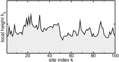
Figure 1: A typical model surface in 1D, $L=100$.

In the latter case, the growth is simulated by the nearest-neighbor rule: $h_{k}(t+1)=h_{k}(t)+\eta_{k}(t)$, if $h_{k}(t)\leq\min\{h_{k-1}(t),h_{k+1}(t)\}$; otherwise, $h_{k}(t+1)=h_{k}(t)$ ($t$ is the time index). The above deposition rule produces surfaces characterized by the universal roughness exponent KTNR00 $\alpha=1/2$. Our objective is to show that it is possible to construct a theoretical probability distribution of deposition events on the surface generated by the above rule. This distribution can then be used to compute measurable quantities at saturation, e.g., the mean density of local minima or maxima. Also, it can serve as the departure point for the construction of other distributions that describe more complex growth processes. Our derivation makes the following two simplifying assumptions. First, we neglect correlations between nearest-neighbor local slopes, which depend on the type of deposition, i.e., the distribution from which $\eta_{k}$ is sampled. Second, we neglect temporal correlations among the groups of the surface configuration classes, as explained later. Because of the above simplifications, our theoretical results for the averages are a mean-field like approximation to the averages measured in simulations.

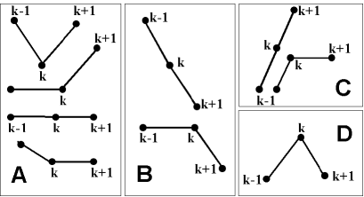
Figure 2: The four groups of elementary local surface configurations at the $k$-th site. In accordance with the adopted growth rule, local A-configuration represents four types of discrete deposition events, and local configuration B (or C) represents two types of events.

The adopted growth rule provides the principle for the classification of local lattice-site configurations of the interface. There are only four groups of these configurations (Fig. 2). Each group corresponds to one of the four mutually exclusive discrete events A, B, C and D that take place at site $k$ during the deposition attempt at $t$: “A” denotes an event when the deposition rule is satisfied from both sides, i.e., $h_{k}(t)\leq h_{k-1}(t)$ and $h_{k}(t)\leq h_{k+1}(t)$; “B” denotes an event when the rule is not satisfied from the right; “C” denotes an event when the rule is not satisfied from the left; “D” denotes an event when the rule is not satisfied from either side. The above events can be mapped in unique way onto elementary local site configurations A, B, C and D, presented in Fig. 2. For a closed chain of sites, the set of events when all sites are simultaneously in the A-configuration is of measure zero, and not all $L$ sites can have the same elementary configuration. Therefore, in the set of $L$ sites there must be at least one site with configuration A. We assign the index $k=1$ to one of the sites in the A-configuration and enumerate the other sites accordingly, progressing to the right. Its right neighbor (site $k=2$) can be only either in configuration C or D. Similarly, its left neighbor (site $k=L$) can be only either in B or D. If site $k=2$ is in C then site $k=3$ can be only either in C or D. If site $k=2$ is in D then site $k=3$ can be only either in B or A. If site $k=3$ is in B then its right neighbor can be either in B or A, etc. Starting from the site $k=1$ and progressing to the right towards $k=L$, applying these elementary neighbor rules, we can construct all possible configuration equivalency classes of the entire surface generated by the adopted growth rule. These can be categorized into groups (called $p$-groups), based on the number $p$ of the deposition events on the surface at $t$, i.e., here, the number of local minima in the surface configuration (coded by “A”) at $t$. The probability distribution $f(p;L)$ of the deposition events is obtained as the quotient of the multiplicity $M(p)$ of the $p$-group and the total number $M$ of configuration classes. (We omit $t$ in the notation since the analysis concerns steady-state evolution.) The mean density $\langle u(L)\rangle$ of local minima is given by the generally valid formula:

$$\langle u(L)\rangle=\sum_{p}u(p)f(p;L)\,,$$ (1)

where the summation is over all $p$-groups of the admissible surface-configuration classes, $u(p)$ is the density characteristic for each group, and $f(p;L)$ is the frequency of the occurrence of the $p$-group at saturation, i.e., the probability of generating a surface with $p$ local minima.

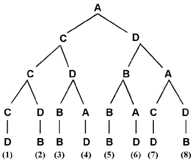
Figure 3: Binary tree for the construction of all possible configuration classes for L=5.

For example, the binary tree for the construction of possible surface-configuration classes for $L=5$ is shown in Fig. 3. Looking along its branches, starting from the leading A at the fixed $k=1$ position, one identifies $M=8$ configuration classes of the entire surface: (1) ACCCD; (2) ACCDB; (3) ACDBB; (4) ACDAD; (5) ADBBB; (6) ADBAD; (7) ADACD; and (8) ADADB. Each surface configuration represents a class of infinitely many topologically equivalent deformations (Fig. 4) since the deposited random height increment is a real positive number. There are only two $p$-groups. In the first, there are four classes with one letter A: $M(1)=4$, $f(1;5)=1/2$, and $u(1)=1/5$. In the second, there are four classes with two letters A: $M(2)=4$, $f(2;5)=1/2$, and $u(2)=2/5$. By Eq. (1), $\langle u(5)\rangle=3/10$.

Figure 4: The graphs of possible surface-configuration classes, corresponding to the configurations read along the branches from Fig. 3 (see text). Each graph represents a class of infinitely many topologically equivalent deformations.

To find $f(p;L)$, one can exploit the recurrent structure of the binary tree for general $L$ in counting classes that contain the A-configuration at exactly $p$ sites KNR03 . Counting gives: $M=2^{L-2}$, $M(p)=(L-1)!/((2p-1)!(L-2p)!)$, and $p=1,2,...,[L/2]$ ($[L/2]=L/2$ for even $L$; $[L/2]=(L-1)/2$ for odd $L$). Thus,

$$f(p;L)=\frac{1}{2^{L-2}}{L-1\choose 2p-1}\,.$$ (2)

In deriving $f(p;L)$ the underlying assumption is that at saturation any class of the entire surface configurations is generated with probability $1/M$. The theoretical $f(p;50)$ is compared with the simulated distributions in Fig. 5. We considered three deposition types: the Poisson type, where $\eta_{k}$ was sampled from the Poisson distribution; Gaussian type, where $\eta_{k}$ was sampled from the Gaussian; and, the uniform deposition with $\eta_{k}$ being a uniform random deviate. In all cases, Eq. (2) is a very close approximation to time-averaged distributions measured in simulations.

Figure 5: Probability distributions for $L=50$: theoretical (histogram), and from simulations with Poisson (circles) and Gaussian (diamonds) depositions. Error bars give one standard deviation from the mean time sequence at saturation. The frequencies were measured in $2048$ independent trials.

Having Eq. (2), all moments of $f(p;L)$ can be computed exactly KNR03 , e.g., for $L\geq 4$ its variance is

$$\sigma^{2}(L)=\sum_{m}\left(m-\langle p(L)\rangle\right)^{2}f(m;L)=\frac{L-1}{16}\,.$$ (3)

For $L\geq 3$ the mean number of local minima is

$$\langle p(L)\rangle=\sum_{m}mf(m;L)=\frac{L+1}{4}\,.$$ (4)

The mean density of local minima, presented in Fig. 6, is simply obtained from Eq. (4) as $\langle u(L)\rangle=\langle p(L)\rangle/L$.

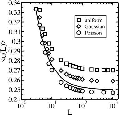
Figure 6: The steady-state mean density $\langle u(L)\rangle$ of local minima vs lattice size $L$. The curve is the analytical result $(L+1)/4L$. The symbols present simulations with the Poisson (circles), Gaussian (diamonds) and uniform (squares) depositions. The error bars are smaller than the symbol size.

Suppose, the adopted growth rule is slightly modified so the deposition at a local minimum (site A) happens with probability $q_{A}$. Then, the new probability distribution $F(n;L,q_{A})$ is the product of the probability $f(n_{A};L)$ of drawing a surface that has exactly $n_{A}$ local minima, given by Eq. (2), and the probability $B(n;n_{A},q_{A})$ that $n$ depositions occur on this surface. The latter is given by binomial distribution

$$B(n;n_{A},q_{A})={n_{A}\choose n}q_{A}^{n}\overline{q}_{A}^{n_{A}-n}\,,$$ (5)

where first factor gives the number of ways in which $n$ depositions can be distributed among $n_{A}$ sites, and $\overline{q}_{A}=1-q_{A}$ is the complementary probability of the no-deposition event at site A. In the old rule: $B(n;n_{A},q_{A}=1)=\delta_{n,n_{A}}$ so, trivially, $F(n;L;q_{A})=f(n_{A};L)$.

Consider next a more complicated rule, where at the $t$-th deposition attempt, the deposition of $\eta_{k}(t)$ is not exclusively confined to local minimum but may also happen at other sites B, C or D with the corresponding probabilities $q_{B}$, $q_{C}$ and $q_{D}$, respectively. We assume now $q_{A}=1$. The probability $F(n;L)\equiv F(n;L;n_{B},n_{C},n_{D};q_{B},q_{C},q_{D})$ of having $n=n_{A}+n_{B}+n_{C}+n_{D}$ deposition sites in the interface is the product:

$$F(n;L) = f(n_{A};L)B(n_{B};N_{B},q_{B})$$ (6)

$$\times B(n_{C};N_{C},q_{C})B(n_{D};N_{D},q_{D})\,.$$

In Eq. (6), $f(n_{A};L)$ is the probability of generating a surface with $n_{A}$ local minima, each of which is the deposition site; the binomial $B(n_{B};N_{B},q_{B})$ is the probability of having $n_{B}$ depositions at $N_{B}$ sites in the local B-configuration on the generated surface; similarly, $B(n_{C};N_{C},q_{C})$ and $B(n_{D};N_{D},q_{D})$ are probabilities that $n_{C}$ and $n_{D}$ depositions occur at $N_{C}$ and $N_{D}$ sites in the local C- and D-configurations, respectively. For any surface, $N_{A}+N_{B}+N_{C}+N_{D}=L$. For surfaces growing on a closed ring of $L$ sites, the number $N_{D}$ of local maxima matches the number $N_{A}$ of local minima. This gives $N_{B}+N_{C}=L-2n_{A}$. By Eq. (1), the mean number $\langle n(L)\rangle$ of deposition sites in the interface is

$$\langle n(L)\rangle=\sum_{n_{A}=1}^{\left[\frac{L}{2}\right]}\sum_{n_{B}=0}^{N_{B}}\sum_{n_{C}=0}^{N_{C}}\sum_{n_{D}=0}^{n_{A}}nF(n;L)\,.$$ (7)

The mean density of these sites is $\langle U(L)\rangle=\langle n(L)\rangle/L$.

In Eq. (7), the summation over $n_{D}$ is easily performed: $\sum_{n_{D}=0}^{n_{A}}(n_{A}+n_{B}+n_{C}+n_{D})B(n_{D};N_{D},q_{D})=n_{A}(1+q_{D})+n_{B}+n_{C}$. This gives

$$\langle n(L)\rangle=\sum_{n_{A}=1}^{\left[\frac{L}{2}\right]}f(n_{A};L)\left(n_{A}\left(1+q_{D}\right)+S_{B\vee C}\right)\,,$$ (8)

where $S_{B\vee C}$ is the mean number of deposition events in the set of sites other than A or D. The computation of $S_{B\vee C}$, though elementary, is a bit tricky since one must distinguish between depositions in the set of B-sites and depositions in the set of C-sites to avoid double counting:

$$S_{B\vee C} = \sum_{n_{B}=0}^{N_{B}}B(n_{B};N_{B},q_{B})\sum_{n_{C}=0}^{N_{C}}B(n_{C};N_{C},q_{C})$$

$$\times (n_{B}+n_{C})=(L-2n_{A})q_{B}q_{C}\,.$$

Substitution to Eq. (8) gives for $L\geq 3$:

$$\langle n(L)\rangle=\frac{1+q_{D}+2\overline{Q}}{4}L+\frac{1+q_{D}-2\overline{Q}}{4}\,,$$ (9)

where $\overline{Q}=1-Q$, $Q=\overline{q}_{B}+\overline{q}_{C}-\overline{q}_{B}\overline{q}_{C}$.

One application of Eq. (9) is the case when $\overline{q}_{B}=\overline{q}_{C}=q/2$ and $\overline{q}_{D}=q$, where the probability $q=\sqrt{2/N}$ is parametrized by an integer $N\geq 2$. Here, the mean density of lattice sites where the deposition takes place is

$$\langle U(L)\rangle=\left(1-\frac{q}{2}\right)\left(1-\frac{q}{4}\frac{L-1}{L}\right)\,.$$ (10)

Predictions of Eq. (10), compared to simulations with the Poisson deposition in Fig. 7, are consistent with the fact that the approximation $f(n_{A};L)$ gives slight overestimates of the density of local minima at the high-$L$ end (Fig. 6). Nevertheless, the analytical $\langle U(L)\rangle$ reflects well the overall tendencies in the data. As $q\to 0$, $\langle U(L)\rangle$ approaches $1$. In this limit-case each attempted deposition event at each lattice site becomes certain. Such a case corresponds to the random deposition growth rule. The corresponding interface is entirely uncorrelated and never saturates. This is the asymptotic limit to which the curves in Fig. 7 converge when $N\to\infty$.

Figure 7: The steady-state mean density $\langle U(L)\rangle$ of deposition sites vs lattice size $L$ when $q$ depends on integer $N\geq 2$: analytical curves of Eq. (10) and the data measured in simulations with the Poisson deposition (symbols).

III OUTLOOK AND CONCLUSION

In summary, we have introduced a new approach for the study of non-universal properties of surfaces. We showed the explicit connection between the interface morphology and the event statistics on the interface at saturation. The key concept here is the ability to build distinct equivalency classes of the entire surface configurations from its local-site configurations. In this construction, the growth rule defines the set of events that can be mapped in a unique way on the set of elementary local-site configurations.

Small differences between simulation results and the approximate analytical results come mainly from neglecting temporal correlations among $p$-groups of surface-configuration classes. These correlations are intrinsically present in the computation of averages over time series in simulations but they are absent in our derivation. They depend on the probability distribution from which the deposited random height increments are sampled. The proper handling of temporal correlations is essential in the microscopic description of the growth phase (before saturation), which is a challenging problem still open. Some insight to this issue may be found in recent works of Rikvold and Kolesik RK , who used the concept of equivalency classes in connecting the interface microstructure with its mobility for Ising and solid-on-solid models with various stochastic dynamics.

Although the focus of the study presented here is on obtaining analytical results in the mean-field spirit, it is interesting to notice the sensitivity of simulation results to the probability distribution used to select random height increments. Negligible variations between the derived analytical probability distribution and simulated distributions with Gaussian, Poissonian and uniform increments demonstrate that the theoretical distribution presents well the statistics of events on the surface. Temporal correlations between interfaces generated via random deposition at local minima deserve further analytical studies.

In conclusion, we observe that our approach could be applied to a variety of other growth rules and models. The current applications to 1D problems are illustrative examples. The main advantage of the approach is that it enables one to compute analytically quantities that can be only estimated qualitatively by continuum methods.

- (1) A.-L. Barabasi and H. E. Stanley, Fractal Concepts in Surface Growth (Cambridge University Press, Cambridge, 1995).
- (2) G. Korniss, Z. Toroczkai, M. A. Novotny, and P. A. Rikvold, Phys. Rev. Lett. 84, 1351 (2000).
- (3) G. Korniss, M. A. Novotny, H. Guclu, Z. Toroczkai, and P. A. Rikvold, Science 299, 677 (2003).
- (4) A. Kolakowska, M. A. Novotny, and P. A. Rikvold, Phys. Rev. E 68, 046705 (2003).
- (5) C.-S. Chin, Phys. Rev. E 66, 021104 (2002).
- (6) Y. Sang, M. Dube, and M. Grant, Phys. Rev. Lett. 87, 174301 (2001).
- (7) V. A. Shneidman, K. A. Jackson, and K. M. Beatty, J. Cryst. Growth 212, 564 (2000).
- (8) P. Meakin, P. Ramanlal, L. M. Sander, and R. C. Ball, Phys. Rev. A 34, 5091 (1986); M. Plischke, Z. Racz, and D. Liu, Phys. Rev. B 35, 3485 (1987).
- (9) F. Family, J. Phys. A 19, L441 (1986).
- (10) P. A. Rikvold and M. Kolesik, J. Stat. Phys. 100, 377 (2000); J. Phys. A: Math. Gen. 35, L117 (2002); Phys. Rev. E 66, 066116 (2002); Phys. Rev. E 67, 066113 (2003).