Disorder and interaction effects in two dimensional graphene sheets

Abstract

The interplay between different types of disorder and electron-electron interactions in graphene planes is studied by means of Renormalization Group techniques. The low temperature properties of the system are determined by fixed points where the strength of the interactions remains finite, as in one dimensional Luttinger liquids. These fixed points can be either stable (attractive), when the disorder is associated to topological defects in the lattice or to a random mass term, or unstable (repulsive) when the disorder is induced by impurities outside the graphene planes. In addition, we analyze mid-gap states which can arise near interfaces or vacancies.

Introduction. Graphite is a widely studied material, which has attracted recent interest due to the observation of anomalous properties, such as magnetism or insulating behavior in the direction perpendicular to the planes in different samplesKopelevich et al. (2000); P. Esquinazi et al. (2002); Kempa et al. (2002); Kopelevich et al. (2002); Moehlecke et al. (2002); Coey et al. (20021); Kopelevich et al. (2003); Kempa et al. (2003).

The conduction band of graphite is well described by tight binding models which include only the $\pi$ orbitals which are perpendicular to the graphite planes at each C atomSlonczewski and Weiss (1958). If the interplane hopping is neglected, this model describes a semi metal, with zero density of states at the Fermi energy, and where the Fermi surface is reduced to two inequivalent points in the Brillouin Zone. The states near these Fermi points can be described by a continuum model which reduces to the Dirac equation in two dimensions. Due the the vanishing of the density of states at the Fermi level, the long range Coulomb interaction is imperfectly screened. This implies that a standard perturbative treatment leads to logarithmic divergences, and to non trivial deviations from Fermi liquid theoryGonzález et al. (1993a); González et al. (1994, 1999). In the strong coupling regime, the model can exhibit a phase transition which leads to a rearrangement of the charges and spins within the unit cell, and which is similar to the chiral symmetry breaking transition found in field theoriesKhveshchenko (2001a, b).

It is known that disorder significantly changes the states described by the two dimensional Dirac equationde C. Chamon et al. (1996); Castillo et al. (1997); Horovitz and Doussal (2002), and, usually, the density of states at low energies is increased. Lattice defects, such as pentagons and heptagons, or dislocations, can be included by means of a non Abelian gauge fieldGonzález et al. (1993b); González et al. (2001). In general, disorder enhances the effect of the interactions. In addition, a graphene plane can show states localized at interfacesWakayabashi and Sigrist (2000); Wakayabashi (2001), which, in the absence of other types of disorder, lie at the Fermi energy. Changes in the local coordination can also lead to localized statesOvchinnikov and Shamovsky (1991).

The present work attempts to study, within the same footing, the role of long range interactions and disorder. This problem has already been studied in relation with critical points between integer and fractional fillings in the Quantum Hall EffectYe and Sachdev (1998); Ye (1999), and we will be able to translate some of the results there to the problem at hand. We find, as inYe (1999) a rich phase diagram, with different fixed points. The stability of these fixed points depends on the nature of the disorder. Finally, we discuss the changes introduced in this picture by the possible existence of localized states near the Fermi edge induced by strong distortions of the lattice.

The model: Coulomb interaction and disorder. We describe the electronic states within each graphene plane by two two-component spinors associated to the two inequivalent Fermi points in the Brillouin Zone. They are combined to a four component (Dirac) spinor. These spinors obey the massless Dirac equation. The Hamiltonian of the free system is:

$$H_{0} =iv_{F}\int d^{2}x\overline{\Psi}(\vec{x})\vec{\gamma}\cdot\vec{\nabla}\Psi(\vec{x})$$ (1)

where $\overline{\Psi}\equiv\Psi^{\dagger}\gamma_{0}$ with the $4\times 4$ matrix $\gamma_{0}\equiv\sigma_{3}\otimes\sigma_{3}$. We further have $\vec{\gamma}\equiv(\gamma_{1},\gamma_{2})=(-i\sigma_{2},i\sigma_{1})\otimes\sigma_{3}$. The $\sigma_{\mu}$ denote the usual Pauli matrices such that $\{\gamma_{\mu},\gamma_{\nu}\}=2g_{\mu,\nu}{\bf{1}}_{4\times 4}$, $g_{\mu,\nu}$ denoting the Minkowski tensor where $g_{0,0}=1$, $g_{i,i}=-1$ with $i=1,2$, and zero otherwise.

The long range Coulomb interaction in terms of the Dirac spinors reads

$$H_{ee} =\frac{v_{F}}{4\pi}\int d^{2}xd^{2}x^{\prime}\overline{\Psi}(\vec{x})\gamma_{0}\Psi(\vec{x})\frac{g}{|\vec{x}-\vec{x}^{\prime}|}\overline{\Psi}(\vec{x}^{\prime})\gamma_{0}\Psi(\vec{x}^{\prime})$$ (2)

where $g=e^{2}/v_{F}$ is the dimensionless coupling constant.

In order to describe disorder effects, the Dirac spinors are coupled to a gauge field $A(\vec{x})$,

$$H_{disorder}=\frac{v_{\Gamma}}{4}\int d^{2}x\overline{\Psi}(\vec{x})\Gamma\Psi(\vec{x})A(\vec{x})$$ (3)

where $v_{\Gamma}$ characterizes the strength and the $4\times 4$ matrix $\Gamma$ the type of the vertex. In general, $A(\vec{x})$ is a quenched, Gaussian variable with the dimensionless variance $\Delta$, i.e.,

$$\langle A(\vec{x})\rangle=0\quad,\quad\langle A(\vec{x})A(\vec{x}^{\prime})\rangle=\Delta\delta^{2}(\vec{x}-\vec{x}^{\prime})\quad.$$ (4)

We will discuss five different types of disorder which are associated to the five mutually anticommuting $4\times 4$ matrices plus the unity matrix: i) For a random chemical potential, the $4\times 4$ matrix $\Gamma$ is given by $\Gamma=\gamma_{0}$. The long range components of this type of disorder do not induce transitions between the two inequivalent Fermi points. This type of disorder will yield an unstable fixed line. ii) A random gauge potential involves the $4\times 4$ matrices $\Gamma=i\gamma_{1}$ and $\Gamma=i\gamma_{2}$. This type of disorder will yield a stable fixed line which is linear in the $(g,\Delta)$-plane. iii) (a) A fluctuating mass term is described by $\Gamma={\bf{1}}_{4\times 4}$. (b) Topological disorder is given by $\Gamma=i\gamma_{5}$ with $\gamma_{5}={\bf{1}}_{2\times 2}\otimes\sigma_{2}$. This type of disorder is associated to the existence of pentagons and heptagons, or, more generally, to local distortions of the lattice axesGonzález et al. (1993b); González et al. (2001). This term can thus be represented by a gauge potential which induces transitions between the two Fermi points. (c) To complete the discussion, we also mention $\Gamma=i\tilde{\gamma}_{5}$ where $\tilde{\gamma}_{5}={\bf{1}}_{2\times 2}\otimes\sigma_{1}$. This vertex type can be related to an imaginary mass that couples the two inequivalent Fermi points. All these types of disorder will yield a stable fixed line which is cubic in the $(g,\Delta)$-plane.

Renormalization of the effective couplings. To discuss the renormalizability of the theory, we will first treat the disorder gauge-field as an external potential and do not consider the average over different realizations of this field. The free, massless Dirac propagator is given byGonzález et al. (1994):

$$G_{0}(\omega,\vec{p}) =-i\int\frac{d\omega}{2\pi}\frac{d^{2}p}{(2\pi)^{2}}e^{i\omega t-i\vec{p}\vec{x}}\langle T\Psi(t,\vec{x})\overline{\Psi}(0,0)\rangle$$

$$=\frac{-1}{\gamma_{0}\omega-v_{F}\vec{\gamma}\cdot\vec{p}+i0}\quad.$$ (5)

Within one loop and without averaging over the disorder potential, only two diagrams need to be considered, i.e., the self-energy of the fermion propagator due to electron-electron interaction and the vertex correction of the “external” gauge field that couples to the Dirac bilinear $\overline{\Psi}\Gamma\Psi$. Both diagrams are shown on the left hand side of Fig. [1].

The Fermi velocity is renormalized by the top left diagram of Fig. [1] as $v_{F}=Z_{v_{F}}\tilde{v}_{F}$ with $Z_{v_{F}}=1-g/(16\pi\varepsilon)$, using dimensional regularization with $\varepsilon\to 0$González et al. (1994). Notice that the vertex of the Coulomb interaction is not renormalized within one-loop order.

Whether or not $v_{\Gamma}$ needs to be renormalized depends on the type of the disorder: i) For a random chemical potential with $\Gamma=\gamma_{0}$, the right diagram at the top of Fig. [1] is non-divergent. This statement is equivalent to the one that there is no vertex correction of the Coulomb interaction. We thus set $v_{\Gamma}=v_{1}$ with the flow-invariant velocity $v_{1}$. ii) For a random gauge potential ($\Gamma=i\gamma_{1},i\gamma_{2}$), the vertex is renormalized by the same factor as the Fermi velocity, i.e., $Z_{\Gamma}=1-g/(16\pi\varepsilon)$. This fact is related to the conservation of the current. We can thus set $v_{\Gamma}=v_{F}$. iii) For a random mass term $\Gamma={\bf{1}}_{4\times 4}$, topological disorder $\Gamma=i\gamma_{5}$, and $\Gamma=i\tilde{\gamma}_{5}$, the vertex strength $v_{\Gamma}$ is renormalized by $Z_{\Gamma}=1-g/(8\pi\varepsilon)$ which follows from i) and ii). Within one loop-level, we can thus set $v_{\Gamma}=v_{F}^{2}/v_{3}$ with the flow-invariant velocity $v_{3}$.

Notice that - irrespective of the type of disorder - our model depends on a single renormalized parameter, $v_{F}$.

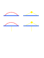
Figure 1: Top: Self energy corrections. Dashed line, Coulomb interaction. Dotted line, ph external disorder. Bottom: Renormalization of the vertex for the external disorder.

Averaging over disorder. As it was discussed in Ref. González et al., 1994, there is no wave function renormalization $Z_{\Psi}$ to leading order in $g$. Including self energy corrections due to averaging over an ensemble of various realizations of the gauge field $A(\vec{x})$, the wave function gets renormalizedGonzález et al. (2001). The self energy due to disorder is shown at the top right of Fig. [1] and reads

$$\Sigma_{\Gamma}(\omega)=\Delta\frac{v_{\Gamma}^{2}}{16}\int\frac{d^{2}p}{(2\pi)^{2}}\Gamma G_{0}(\omega,\vec{p})\Gamma\quad.$$ (6)

The wave function renormalization is independent of the vertex type and yields $Z_{\Psi}=1-\Delta v_{\Gamma}^{2}/(32\pi v_{F}^{2}\varepsilon)$, where again we use dimensional regularization with $\varepsilon\to 0$.

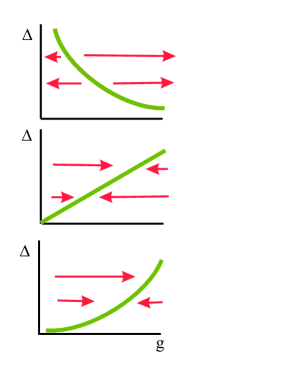
Figure 2: One-loop phase diagram for two-dimensional massless Dirac spinors including long-ranged electron-electron interaction $g$ and disorder $\Delta$. Top: Random chemical potential ($\Gamma=\gamma_{0}$). Center: Random gauge potential ($\Gamma=i\gamma_{1},i\gamma_{2}$). Bottom: Random mass term ($\Gamma={\bf{1}}_{4\times 4}$), topological disorder ($\Gamma=i\gamma_{5}$), and $\Gamma=i\tilde{\gamma}_{5}$.

The wave function renormalization $Z_{\Psi}$ also changes the renormalization factor of the Fermi velocity as we keep $G_{0,Z}^{-1}-\Sigma$ invariant with

$$G_{0,Z}^{-1}(\omega,\vec{p})\equiv-Z_{\Psi}(\gamma_{0}\omega-Z_{v_{F}}v_{F}\vec{\gamma}\cdot\vec{p})\quad.$$ (7)

We also need to discuss the vertex corrections due to averaging over the disorder. The diagram which renormalizes the vertex of the external gauge field is shown at the bottom of Fig. [1]. Also the vertex of the Coulomb interaction is being renormalized (not shown). The vertex correction to $\Gamma$ due to averaging over the disorder type $\Gamma^{\prime}$ is given by

$$V_{\Gamma}(\omega,\vec{k})=\Delta\frac{v_{\Gamma^{\prime}}^{2}}{16}\int\frac{d^{2}p}{(2\pi)^{2}}\Gamma^{\prime}G_{0}(\omega,\vec{p})\Gamma G_{0}(\omega,\vec{p}+\vec{k})\Gamma^{\prime}.$$ (8)

This expression depends on the given combination of vertices, but does not result in a renormalization of the electric charge ($\Gamma=\gamma_{0}$). In the case, where there is only one type of disorder, the vertex correction exactly compensates the effect of $Z_{\psi}$ on $Z_{v_{F}}$ such that the relation between $v_{\Gamma}$ and $v_{F}$ remains valid, i.e., i) $v_{\Gamma}=v_{1}$, ii) $v_{\Gamma}=v_{F}$, and iii) $v_{\Gamma}=v_{F}^{2}/v_{3}$ with $v_{1},v_{3}$ constant.

Phase diagrams. Disorder thus only changes the flow of the Fermi velocity due to wave function renormalization, i.e., $Z_{v_{F}}\to Z_{v_{F}}/Z_{\Psi}$. From the beta-function $\beta_{v_{F}}=\Lambda\partial_{\Lambda}Z_{v_{F}}\tilde{v}_{F}$, we obtain the following flow equation for the effective Fermi velocity $v_{F}^{eff}$ ($\ell=\ln\Lambda/\Lambda_{0}\sim 1/\varepsilon$):

$$\frac{d}{d\ell}\frac{v_{F}^{eff}}{\tilde{v}_{F}}=\frac{1}{16\pi}\left[\frac{e^{2}}{v_{F}^{eff}}-\frac{\Delta}{2}\left(\frac{v_{\Gamma}^{eff}}{v_{F}^{eff}}\right)^{2}\right]$$ (9)

We can now discuss the phase diagram for the various types of disorder: i) For a random chemical potential $(\Gamma=\gamma_{0})$, $v_{\Gamma}=v_{1}$ remains constant under renormalization group transformation. There is thus an unstable fixed line at $v_{F}^{*}=v_{1}^{2}\Delta/(2e^{2})$. In the $(g,\Delta)$-plane, the strong-coupling and the weak-coupling phases are separated by a hyperbola, with the critical electron interaction $g^{*}=e^{2}/v_{F}^{*}=2e^{4}/(v_{1}^{2}\Delta)$. ii) A random gauge potential involves the vertices $\Gamma=i\gamma_{1},i\gamma_{2}$. The vertex strength renormalizes as $v_{\Gamma}=v_{F}$. There is thus an attractive Luttinger-like fixed point for each disorder correlation strength $\Delta$ given by $v_{F}^{*}=2e^{2}/\Delta$ or $g^{*}=\Delta/2$. iii) For a random mass term $\Gamma={\bf{1}}_{4\times 4}$, topological disorder $\Gamma=i\gamma_{5}$, and $\Gamma=i\tilde{\gamma}_{5}$, we have $v_{\Gamma}=v_{F}^{2}/v_{3}$. There is thus again an attractive Luttinger-like fixed point for each disorder correlation strength $\Delta$ given by $v_{F}^{*}=\root 3 \of{2v_{3}^{2}e^{2}/\Delta}$ or $g^{*}=\root 3 \of{\Delta e^{4}/(2v_{3}^{2})}$.

To make connection to previous workYe (1999), we define $\widetilde{\Delta}\equiv\frac{\Delta}{2}(v_{\Gamma}^{eff}/v_{F}^{eff})^{2}$. This yields the linear fixed line $g^{*}=\widetilde{\Delta}$ with i) $\widetilde{\Delta}\propto g^{2}$, ii) $\widetilde{\Delta}\propto\text{const.}$, and iii) $\widetilde{\Delta}\propto g^{-2}$. For one disorder type, our results thus agree with the ones by Ye.

Localized states. The tight binding model defined by the $\pi$ orbitals at the lattice sites can have edge states when the sites at the edge belong all to the same sublatticeWakayabashi and Sigrist (2000); Wakayabashi (2001); Yamashiro et al. (2003). These states lie at zero energy, which, for neutral graphene planes, correspond to the Fermi energy. The states at zero energy are localized in one of the two interpenetrating sublattices which can be defined in the honeycomb structure. In terms of each of the two component spinors, in the continuum approximation used here, a possible state localized in one edge can be written as $\Psi({\bf\vec{r}})\equiv A(e^{ikz},0)$, where $z=x+iy$, we assume that the edge lies at $y=0$, and that the graphene fills the upper half plane, $y\geq 0$.

In a strongly disordered sample, large defects made up of many vacancies can exist. These defects give rise to localized states, when the termination at the edges is locally similar to the surfaces discussed above. Note that, if the bonds at the edges are saturated by bonding to other elements, like hydrogen, the states at these sites are removed from the Fermi energy, but a similar boundary problem arises for the remaining $\pi$ orbitals. A particular simple example is given by the crack shown in Fig.[3]. The boundary conditions are such that $\Psi(z)\equiv[f(z),0]$ where $f(z)=0$ at the surface of the crack, because it has edges of the two sublattice types. Possible edge states are: $\Psi_{n}\equiv\left\{{\rm Re}\left[\frac{A}{z^{n}\sqrt{z^{2}-a^{2}}}\right],0\right\}$. A similar solution is obtained by exchanging the upper by the lower spinor component, and replacing $z\leftrightarrow\bar{z}$. Because of the discreteness of the lattice, the values of $n$ should be smaller than the number of lattice units spanned by the crack.

These states are half filled in a neutral graphene plane. In the absence of electron interactions, this leads to a large degeneracy in the ground state. A finite local repulsion will tend to induce a ferromagnetic alignment of the electrons occupying these states, as in similar cases with degenerate bandsVollhardt et al. (1999). Hence, we can assume that the presence of these states leads to magnetic moments localized near the defects.

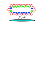
Figure 3: Top: example of a crack in a graphene plane. The atoms at the upper edge and those at the lower edge belong to different sublattices. Bottom: approximate cut in the complex plane which can be used to represent this crack at long distances. See text for details.

We now have to analyze the influence of these magnetic moments in conduction band described in the previous sections. The hopping between the states involved in the formation of these moments and the delocalized states in the conduction band vanishes when the localized states lie at zero energy. Hence, an antiferromagnetic Kondo coupling will not be induced. The localized and conduction band states, on the other hand, coexist at the same lattice sites. The presence of a finite local repulsion, $U$, will lead to a ferromagnetic coupling. The local coupling, at site $i$, between the localized states and the conduction band is proportional to $U\sum_{j}\rho_{i,j}$, where $\rho_{i,j}$ is charge of state $j$ at site $i$. The conduction electrons will mediate an RKKY interaction between the localized moments:

$$J_{RKKY}({\bf\vec{r}})\sim U^{2}\int d^{2}{\bf k}e^{i{\bf\vec{k}}{\bf\vec{r}}}\chi({\bf\vec{k}})\sim U^{2}\frac{a^{4}}{v_{F}|{\bf\vec{r}}|^{3}}$$ (10)

Where the static susceptibility is $\chi({\bf\vec{k}})\propto|{\bf\vec{k}}|$González et al. (1997), and $a$ is the lattice constant. It is interesting to note that, due to the absence of a finite Fermi surface, the RKKY interaction in eq.(10) does not have oscillations. Hence, there are no competing ferro- and antiferromagnetic couplings, and the magnetic moments will tend to be ferromagnetically aligned. Asuming $U\sim\hbar v_{F}/a\sim 1-3$eV, this argument leads to a Curie temperature $T_{C}\sim U\langle a^{3}/d^{3}\rangle$, where $d$ is the distance between defects.

Conclusions. In this work, we estimated the effect of disorder in graphene sheets in the presence of long-ranged electron-electron interaction. The disorder term can be characterized by five different vertices which lead - within a one-loop level - to three distinct phase diagrams. A random chemical potential divides the phase diagram into a strong-coupling and weak-coupling regime by an unstable fixed line. A random gauge potential as well as a random mass term and topological disorder alter the electronic structure of two-dimensional graphene sheets as it drives the system towards a stable, Luttinger-like fixed point. As extensively analyzed previously (see, for instanceGonzález et al. (1999)) the dimensionless Coulomb coupling, for graphene planes is $g=e^{2}/(\epsilon_{0}v_{F})\sim 1$. Randomness in the chemical potential, due to local defects, like impurities or vacancies, lead to $\Delta\sim(V/\hbar v_{F})^{2}c$, where $V$ is the strength of the local potential and $c$ is the concentration ($\Delta\sim ca^{2}$ for vacancies, where $a$ is the lattice constant). Lattice defects, such as inclinations or disclinations, induce an effective gauge potential, whose strength, for dislocations, can be expressed as $\Delta\sim cb^{2}$González et al. (2001), where $b$ is the Burgers vector of the dislocation. The actual strength of the disorder, however, can be much larger for experiments performed on irradiated samplesh. Han et al. (2003). Hence, it is likely that graphene sheets are in the intermediate range coupling, and we can expect a qualitative behavior like that reported here. Note that the presence of disorder at intermediate scales will suppress the chiral symmetry breaking transition expected for pure grapheneKhveshchenko (2001a, b).

Acknowledgments. T.S. is supported by the DAAD-Postdoctoral program. Funding from MCyT (Spain) through grant MAT2002-0495-C02-01 is also acknowledged. M.A.H.V. thanks A. Ludwig and C. Mudry for very useful conversations on disordered systems. We also thank P. Esquinazi for many illuminating discussions.

References

- Kopelevich et al. (2000) Y. Kopelevich, P. Esquinazi, J. H. S. Torres, and S. Moehlecke, J. Low Temp. Phys. 119, 691 (2000).
- P. Esquinazi et al. (2002) A. S. P. Esquinazi, R. Höhne, C. Semmelhack, Y. Kopelevich, D. Spemann, T. Butz, B. Kohlstrunk, and M. Lösche, Phys. Rev. B 66, 024429 (2002).
- Kempa et al. (2002) H. Kempa, P. Esquinazi, and Y. Kopelevich, Phys. Rev. B 65, 241101 (2002).
- Kopelevich et al. (2002) Y. Kopelevich, P. Esquinazi, J. H. S. Torres, R. R. da Silva, H. Kempa, F. Mrowka, and R. Ocana (2002), eprint cond-mat/0209442.
- Moehlecke et al. (2002) S. Moehlecke, P.-C. Ho, and M. B. Maple, Phil. Mag. Lett (2002).
- Coey et al. (20021) J. M. D. Coey, M. Venkatesan, C. B. Fitzgerald, A. P. Douvalis, and I. S. Sanders, Nature 420, 156 (20021).
- Kopelevich et al. (2003) Y. Kopelevich, J. H. S. Torres, R. R. da Silva, F. Mrowka, H. Kempa, , and P. Esquinazi, Phys. Rev. Lett. 90, 156402 (2003).
- Kempa et al. (2003) H. Kempa, H. C. Semmelhack, P. Esquinazi, and Y. Kopelevich, Solid State Commun. 125, 1 (2003).
- Slonczewski and Weiss (1958) J. C. Slonczewski and P. R. Weiss, Phys. Rev. 109, 272 (1958).
- González et al. (1993a) J. González, F. Guinea, and M. A. H. Vozmediano, Mod. Phys. Lett. B7, 1593 (1993a).
- González et al. (1994) J. González, F. Guinea, and M. A. H. Vozmediano, Nucl. Phys. B 424 [FS], 595 (1994).
- González et al. (1999) J. González, F. Guinea, and M. A. H. Vozmediano, Phys. Rev. B 59, R2474 (1999).
- Khveshchenko (2001a) D. V. Khveshchenko, Phys. Rev. Lett. 87, 246802 (2001a).
- Khveshchenko (2001b) D. V. Khveshchenko, Phys. Rev. Lett. 87, 206401 (2001b).
- de C. Chamon et al. (1996) C. de C. Chamon, C. Mudry, and X.-G. Wen, Phys. Rev. B 53, R7638 (1996).
- Castillo et al. (1997) H. E. Castillo, C. de C. Chamon, E. Fradkin, P. M. Goldbart, and C. Mudry, Phys. Rev. B 56, 10668 (1997).
- Horovitz and Doussal (2002) B. Horovitz and P. L. Doussal, Phys. Rev. B 65, 125323 (2002).
- González et al. (1993b) J. González, F. Guinea, and M. A. H. Vozmediano, Nucl. Phys. B 406 [FS], 771 (1993b).
- González et al. (2001) J. González, F. Guinea, and M. A. H. Vozmediano, Phys. Rev. B 63, 134421 (2001).
- Wakayabashi and Sigrist (2000) K. Wakayabashi and M. Sigrist, Phys. Rev. Lett. 84, 3390 (2000).
- Wakayabashi (2001) K. Wakayabashi, Phys. Rev. B 64, 125428 (2001).
- Ovchinnikov and Shamovsky (1991) A. A. Ovchinnikov and I. L. Shamovsky, Journ. of. Mol. Struc. (Theochem) 251, 133 (1991).
- Ye and Sachdev (1998) J. Ye and S. Sachdev, Phys. Rev.Lett. 80, 5409 (1998).
- Ye (1999) J. Ye, Phys. Rev. B. 60, 8290 (1999).
- Yamashiro et al. (2003) A. Yamashiro, Y. Shimoi, K. Harigaya, and K. Wakabayashi (2003), eprint cond-mat/0309363.
- Vollhardt et al. (1999) D. Vollhardt, N. Blümer, K. Held, M. Kollar, J. Schlipf, M. Ulmke, and J. Wahle, in Advances in Solid State Physics (Wieweg, 1999).
- González et al. (1997) J. González, F. Guinea, and M. A. H. Vozmediano, Phys. Rev. Lett. 77, 3589 (1997).
- h. Han et al. (2003) K. h. Han, D. Spemann, P. Esquinazi, R. Höhne, R. Riede, and T. Butz, Adv. Mat. (2003).