Vortex nucleation and flux front propagation in type II superconductors

Abstract

We study flux penetration in a disordered type II superconductor by simulations of interacting vortices, using a Monte Carlo method for vortex nucleation. Our results show that a detailed description of the nucleation process yields a correction to the scaling laws usually associated with flux front invasion. We propose a simple model to account for these corrections.

1 Introduction

The magnetization of type II is traditionally described in terms of the Bean model bean : magnetic flux enters into the sample from the boundaries, forming a flux gradient that is pinned by disorder. At the microscopic level, the process takes place through the nucleation of vortex lines carrying each a flux quantum Blatter . The Bean model provides a phenomenological picture of average magnetization properties, such as hysteresis and thermal relaxation kim , but it is inadequate to describe fluctuations, which turn out to be quite important. As it has been shown experimentally using magnetoptical methods, flux fronts are typically rough or even fractal rough ; fractal ; fractal2 .

Recently, we have shown that the flux penetration in a disordered superconductor can be described by a disordered non-linear diffusion equation zms . The equation can be obtained performing a coarse-graining of the microscopic equation of motion of the vortices. In the absence of pinning, it reduces to the model introduced in Ref. dorog . This model has been solved analytically to provide expressions for the dynamics of the front for different boundary conditions dorog ; gilc and the results are in perfect agreement with vortex dynamics simulations MOR-02 . When quenched disorder is included in the diffusion equations, flux fronts are pinned in agreement with individual vortex simulations. Varying the parameters of the equation, we observe a crossover from flat to fractal flux fronts, consistent with experimental observations. The value of the fractal dimension suggests that the strong disorder limit is described by gradient percolation zms .

Here we reconsider the influence of boundary conditions in the front dynamics. In Ref. MOR-02 we have analyzed several types of boundary conditions determining the way vortices enter into the sample depending of the experimental setup one would like to model. For instance, a constant applied magnetic field can be approximated by a constant vortex density at the boundary of the sample dorog ; gilc . This assumption simplifies the real vortex nucleation process and allows for straightforward numerical and analytical approaches zms ; dorog ; gilc ; MOR-02 . A more accurate description of vortex nucleation can be obtained combining the vortex dynamics simulations with the Monte Carlo method SHU-97 . Using this method we find that the simple widely employed approximations for the boundary conditions are only asymptotically true. At short times the details of the nucleation process affects the expected scaling behavior for the front dynamics. We are able to quantitatively estimate the corrections to scaling, using a simple front dynamics model in the spirit of Washburn approach to fluid imbibition dube

2 Simulations

We use here the model introduced in Ref. SHU-97 , which combines a typical vortex dynamics simulation scheme with a Monte Carlo method for vortex nucleation. In a very large sample with a constant magnetic field $H$ oriented along the $z$ axis, vortices are modeled as a set of interacting particles performing an overdamped motion in the $xy$ plane.

The Gibbs potential associated to $N$ vortices of coordinates $\vec{r}_{i}$ can be written as

$$G=\sum_{ij}E_{12}(\vec{r}_{i}-{r}_{j})+\sum_{i}\tau_{i}(x_{i})-\frac{H}{4\pi}\sum_{i}\phi_{i}(x_{i}),$$ (1)

where in an infinite system $E_{12}(\vec{r})=[\Phi_{0}^{2}/(8\pi^{2}\lambda^{2})]K_{0}(|\vec{r}|/\lambda)$ is the vortex-vortex interaction in the London-London theory, with flux quantum $\Phi_{0}$ and penetration length $\lambda$. Here we consider a semi-infinite system, bounded by the $y=0$ line, and consequently we add to the vortex-vortex interaction a term accounting for the interaction between each vortex and the image of the others SHU-97 . The term $\tau_{i}(x_{i})$, where $x_{i}$ is the distance between the vortex $i$ and the sample surface, represents the interaction between each vortex and its own image SHU-97 . Finally the external magnetic field gives rise to a sort of chemical potential with $\phi(x)\equiv\Phi_{0}(1-\exp(-x/\lambda)$. In Ref. SHU-97 the interaction energy with random pinning centers is also included to Eq. 1, while here we restrict our attention to a clean system.

The vortices evolve according to an overdamped equation of motion $\Gamma\partial_{t}\vec{r}_{i}=-\partial_{r_{i}}G$, where $\Gamma$ is a damping constant. The equation of motion is integrated numerically and after each integration step a zero temperature Monte Carlo step is performed: a new vortex is nucleated at a random position in a strip of length $\lambda$ close to the sample boundary if the Gibbs potential is reduced. In practice, we consider a system of size $L_{y}=20\lambda$ and $L_{x}=100\lambda$, with periodic boundary conditions along the $y$ direction. At the beginning of the simulation, we start with an empty lattice and vortices are nucleated close to the $x=0$ boundary. Since we are only interested in the transient behavior the boundary condition at $x=L_{x}$ is inessential.

As the vortices are nucleated, they are pushed toward the interior of the sample giving rise to a density profile. The evolution of the profile is reported in Fig. 1. The results are in slight disagreement with the simplified boundary condition used in Refs. dorog ; gilc ; MOR-02 : a constant boundary vortex density. Fig. 1 clearly shows that the boundary density increases. In addition, Fig. 2 shows that the front position does not evolves as a power law, $x_{p}\sim t^{1/2}$, as predicted by the theory dorog ; gilc ; MOR-02 .

Figure 1: The density profile at different times $t$ obtained from numerical simulations.

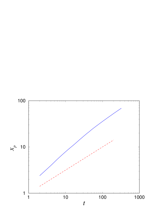
Figure 2: The position of the front at different times $t$ obtained from numerical simulations. The dashed line is the $t^{1/2}$ prediction

3 A simple model for front dynamics

In order to account for the behavior observed in numerical simulations, we consider a simple model for the front dynamics MOR-02 . The front is driven by the density gradient which can be can be estimated simply as $\nabla\rho\simeq\rho_{0}/x_{p}$, where $x_{p}$ is the front position and $\rho_{0}=\rho(0,t)$ is the boundary density. Thus the equation of motion of the front can be written as $\Gamma dx_{p}/dt=a\rho_{0}/x_{p}$, where $a$ is the interaction parameter computed in Ref. MOR-02 . In order to solve this equation, we have to specify the dynamics of the boundary density, which to a first approximation can be written as $\tau d\rho_{0}/dt=\rho_{H}-\rho_{0}$ where $\rho_{H}\propto H$ is the asymptotic value of the vortex density, and $\tau$ a characteristic time.

Solving the two differential equations, we obtain

$$\rho_{0} = \rho_{H}(1-\exp(-t/\tau))$$ (2)

$$x_{p}(t) = \left(\frac{2a\rho_{H}}{\Gamma}\right)^{1/2}(t+\tau(1-\exp(-t/\tau)))^{1/2}.$$ (3)

In order to compare this result with numerical simulations, we plot on the same graph the numerically calculated $\rho_{0}$ and $dx_{p}^{2}/dt$ together with the theoretical prediction from Eq. 2. The numerical result can be well fit by the model with $\tau\simeq 10$.

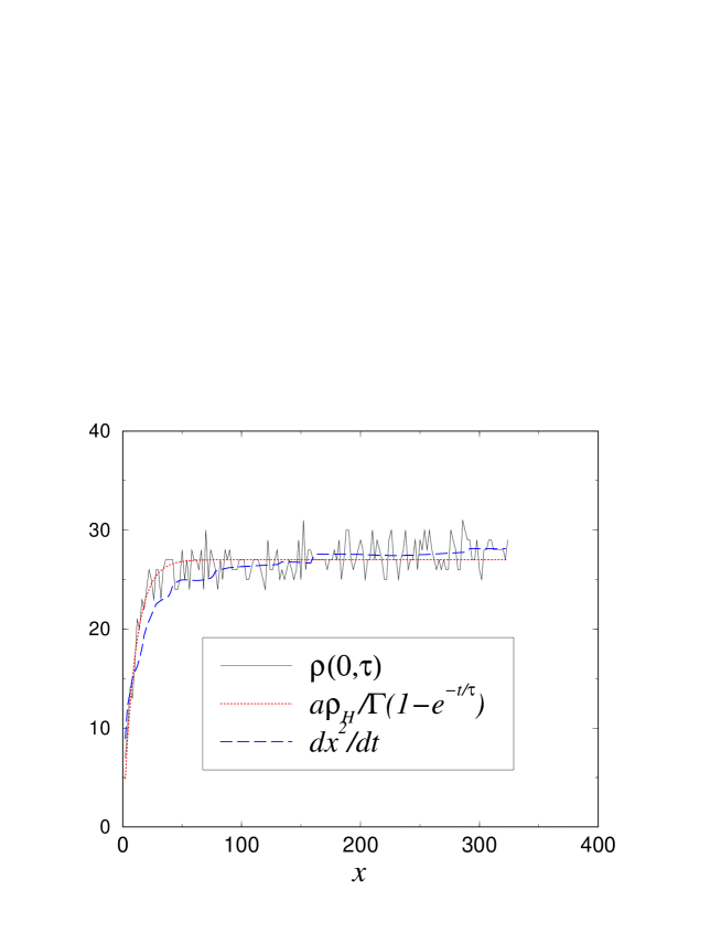
Figure 3: A comparison between the front dynamics model and the numerical simulations.

4 Conclusions

In this paper we have considered the effect of vortex nucleation on flux front propagation in type II superconductors. We have studied the case of a constant applied magnetic field and compared the results of numerical simulations with previous approaches to the problem dorog ; gilc ; MOR-02 . While asymptotically we recover previous results, a more accurate account of the vortex nucleation process leads to important corrections for the scaling laws. This fact should be considered in the interpretation of experimental results.

References

- (1) C. P. Bean, Rev. Mod. Phys. 36, 31 (1964).
- (2) G. Blatter, M.V. Feigel’man, V.B. Geshkenbein, A.I. Larkin, and V.M. Vinokur, Rev. Mod. Phys. 66, 1125 (1994).
- (3) Y. B. Kim, C. F. Hempstead and A. R. Strnad, Phys. Rev. 129, 528 (1963).
- (4) R. Surdeanu, R. J. Wijngaarden, E. Visser, J. M. Huijbregtse, J. H. Rector, B. Dam, and R. Griessen Phys. Rev. Lett. 83, 2054 (1999).
- (5) R. Surdeanu, R. J. Wijngaarden, B. Dam, J. Rector, R. Griessen, C. Rossel, Z. F. Ren, and J. H. Wang, Phys. Rev. B 58, 12467 (1998).
- (6) S. S. James, S. B. Field, J. Seigel and H. Shtrikman, Physica C 332, 445 (2000).
- (7) S. Zapperi, A. A. Moreira, J. S. Andrade Jr., Phys. Rev. Lett. 86, 3622 (2001).
- (8) A. A. Moreira, J. S. Andrade Jr., J. Mendes Filho and S. Zapperi Phys. Rev. B 66, 174507 (2002).
- (9) V. V. Bryskin and S. N. Dorogotsev, JEPT 77, 791 (1993); Physica C 215, 173 (1993).
- (10) J. Gilchrist and C. J. van der Beek, Physica C 231, 147 (1994).
- (11) J. Shumway and S. Satpathy, Phys. Rev. B 56, 103 (1997).
- (12) E. Washburn, Phys. Rev. 17, 273 (1921). For a review see M. Dube, M. Rost and M. Alava, Eur. Phys. J. B 15, 691 (2000).