Scaling of star polymers: high order results

Abstract

We extend existing renormalization group calculations for the exponents describing scaling of star polymers and polymer networks constituted by chains of different species (the so-called copolymer star exponents). Our four loop results find application in the description of various phenomena involving self-avoiding and random walks that interact.

1 Introduction

Star polymers, i.e. structures of polymer chains that are chemically linked with one end to a common core attain recently much attention both in theory, experiment, and technical applications [2]. On the experimental side this is due to their effective interaction properties that interpolate between those of colloidal particles and single chain polymers. For theory and simulation they present the most simple albeit non-trivial examples of polymeric networks which, as shown by theory, provide all information to derive the scaling properties of general polymer networks. For this reason the scaling properties of stars of long flexible polymer chains in a good solvent are of central interest [3, 4]. The scaling of single long flexible polymer chains is perfectly described by a model of self-avoiding walks resulting in universal scaling exponents that only depend on the space dimension $d$ [5]. However, the corresponding scaling exponents for star polymers will also depend on the number of arms $f$ constituting the star [3]. Building a polymer star from chains of different species one finds an even richer scaling behavior [6, 7]. The partition function of such a so-called copolymer star consisting of $f_{1}$ chains of species 1 and $f_{2}$ chains of species 2 (each of the same size $R$) will show power law scaling in $R$ according to [7]:

$${\mathcal{Z}}^{(*f_{1}f_{2})}\sim(R/\ell)^{\eta_{f_{1}f_{2}}-f_{1}\eta_{20}-f_{2}\eta_{02}},$$ (1)

with a family of copolymer star exponents $\eta_{f_{1}f_{2}}$ for $f_{1},f_{2}=0,1,2,\ldots$. In (1) $\ell$ is a microscopic scale and a fugacity factor is omitted. We consider a species A of self- and mutually avoiding chains (SAW), species B and B^′ of both self and mutually transparent chains (RW) and a species C of self-transparent but mutually avoiding chains (MAW). Copolymer stars are built from one or more of these species with mutual avoidance between any two species. Of special interest are the exponents of (a) homogeneous polymer stars $\eta^{S}_{f_{A}}$, (b) symmetric and unsymmetric copolymer stars $\eta^{G}_{f_{B}f_{B^{\prime}}}$ and $\eta^{U}_{f_{A}f_{B}}$, and (c) of stars of mutually avoiding walks $\eta^{MAW}_{f_{C}}$. These exponents naturally arise when describing e.g. the scaling properties of the effective interaction of star polymers, the correlations of the vertices of a branched polymeric structure, the diffusion of particles near an absorbing polymer, and the transition of double stranded to single stranded DNA [2, 8, 9]. Moreover, the star exponents $\eta_{f_{A}f_{B}}$ uniquely define the scaling of copolymer networks of arbitrary but fixed topology [3, 4, 7]. The above mentioned facts together with theoretical reasons (e.g. the copolymer star exponents are related to the composite operators of polymer field theory and possess multifractal properties [10] which seemingly is in contradiction with stability conditions [11]) explain the high interest in their analysis.

Currently, the field theoretical renormalization group (RG) [12] is recognized as the most reliable analytic tool to calculate numerical values of scaling exponents in a systematic perturbative way. For the universality class of $O(m)$-symmetric $\phi^{4}$ theory exponents are known up to high orders of perturbation theory: to the 5th order in $\varepsilon=4-d$ expansion [13] and to the 6th/7th order when calculated directly at fixed space dimension $d=3$ [14]. However, the star exponents are known so far only to the 3rd order of perturbation theory [4, 7]. A principal reason for this gap is that copolymer star exponents were introduced only recently [7] and that these exponents have no direct counterparts in the theory of magnets.

Our main message is given by the analytic expressions for the copolymer star exponents that we obtained by state-of-the-art RG methods to $\varepsilon^{4}$ accuracy in an $\varepsilon$-expansion. This is merely one order below the best known $\varepsilon$-expansion for the critical exponents of the $m$-vector model [13]. When evaluated numerically [15, 16] by appropriate resummation techniques [12] the expansions for the exponents lead to results in nice correspondence with the available exact (2D) and MC data. This paper is organized as follows: the next, 2nd section introduces the main expressions relating the copolymer star exponents to polymer field theory, section 3 presents the $\varepsilon$-expansions for the three cases discussed above: $\eta^{G}_{f_{B}f_{B^{\prime}}}$, $\eta^{U}_{f_{A}f_{B}}$ and $\eta^{MAW}_{f_{C}}$. In the last section we conclude and discuss our results presenting a numerical estimate drawn from our expansions. Details of our calculations along with numerical estimates of different quantities involving star exponents are the subject of a separate publication [15].

2 The renormalization group relations

Here, we sketch the framework of polymer field theory suited to describe copolymer stars. The starting point is the Edwards model [5] generalized to describe a set of $f_{1}+f_{2}$ polymer chains in solution with self- and mutual- avoiding interactions $u_{ab}$. Within this model, the configuration of each chain $a=1,\dots,f_{1}+f_{2}$ is given by a path $r^{a}(s)$ in $d$-dimensional space, $0\leq s\leq S_{a}$, $S_{a}$ is the so-called Gaussian surface of the path $r^{a}(s)$. The Hamiltonian ${\mathcal{H}}_{f_{1}f_{2}}$ of the model reads [4, 7]:

$$\frac{1}{k_{\rm B}T}{\mathcal{H}}_{f_{1}f_{2}}({\bf r}^{a},\{S_{a}\})=\sum_{a=1}^{f_{1}+f_{2}}\int_{0}^{S_{a}}{\rm d}s(\frac{{\rm d}{\bf r}^{a}(s)}{2{\rm d}s})^{2}+\frac{1}{6}\sum_{a,b=1}^{f_{1}+f_{2}}u_{ab}\int{\rm d}{\bf r}\rho_{a}({\bf r})\rho_{b}({\bf r}),$$ (2)

with densities $\rho_{a}({\bf r})=\int_{0}^{S_{a}}{\rm d}s\delta({\bf r}-{\bf r}^{a}(s))$. In Eq. (2), the first term describes the chain connectivity whereas the second one stands for the excluded volume interaction. The partition function of a star of $f_{1}+f_{2}$ polymer chains ${\mathcal{Z}}^{(*f_{1}f_{2})}$ is calculated as a functional integral ($\int{\mathcal{D}}[{\bf r}_{a}]$) of the Boltzmann distribution with the Hamiltonian (2) over all possible configurations of the paths $r^{a}(s)$. A product of $\delta$-functions serves as a constraint ensuring all polymer chains to have a common endpoint:

$${\mathcal{Z}}^{(*f_{1}f_{2})}\{S_{a}\}=\int{\mathcal{D}}[{\bf r}_{a}]\exp\{-\frac{1}{k_{\rm B}T}{\mathcal{H}}_{f_{1}f_{2}}({\bf r}_{a},\{S_{a}\})\}\prod_{a=2}^{f_{1}+f_{2}}\delta({\bf r}_{a}(0)-{\bf r}_{1}(0)).$$ (3)

The mapping of the Edwards model to a $\phi^{4}$ field theory with one coupling of $O(m)$-symmetry in the limit $m=0$ is well established [5]. The polymer system we are currently interested in is the so-called ternary polymer solution, where polymer chains of two species (1 and 2) are present. It is described by an Edwards model (2) with three couplings [17]:

$$u_{ab}=\{u_{11},u_{22},u_{12}=u_{21}\}.$$ (4)

The partition function of the copolymer star (3) corresponds in the field theory to a vertex function with the insertion of a composite operator $\Pi_{a}\phi_{a}$ of a special symmetry [7]. Ultraviolet divergences occur when the bare vertex functions are evaluated naively [12]. We apply the field theoretical RG approach [7] to remove the divergences and to study the scaling properties of the vertex functions of copolymer stars. Since the theory is renormalizable one can collect all divergences in the so-called renormalization factors $Z$ and define a finite theory with renormalized parameters preserving the structure of the original one. The renormalized couplings $g_{ab}$ and the renormalization factors $Z$ depend on the parameter $\kappa$ which gives the scale of the external momenta in the renormalization procedure. This dependence is expressed by RG functions defined by the following relations:

$$\kappa\frac{\rm d}{{\rm d}\kappa}{g}_{aa} = {\beta}_{aa}(g_{aa}),\hskip 30.00005pta=1,2,$$ (5)

$$\kappa\frac{\rm d}{{\rm d}\kappa}{g}_{12} = {\beta}_{12}(g_{11},g_{22},g_{12}),$$ (6)

$$\kappa\frac{\rm d}{{\rm d}\kappa}\ln Z_{*f_{1}f_{2}} = \eta_{f_{1}f_{2}}(g_{11},g_{22},g_{12}).$$ (7)

In Eq. (7), $Z_{*f_{1}f_{2}}$ stands for the $Z$-factor renormalizing the vertex function of a composite operator, which corresponds to the copolymer star partition function (3). In the fixed points of the RG transformation, given by a common zero of the $\beta$-functions (5), (6) the anomalous dimensions $\eta_{f_{1}f_{2}}$ of the composite operators define the set of exponents for copolymer stars. Explicit expressions for the star exponents will be given in the next section.

3 $\varepsilon^{4}$-expansions for the exponents

The zeros of the $\beta$-functions (5), (6) correspond to the fixed points of the theory. To clarify their physical significance we here refer to the three classes of species A, B, and C introduced above and denote nontrivial values by $g^{*}_{S}$, $g^{*}_{G}$, and $g^{*}_{U}$. The fixed points of (5) are $\beta_{11}(g^{*}_{S})=0$ for species A, $\beta_{aa}(0)=0$ for species B and C. The non-trivial fixed points of (6) are $\beta_{12}(0,0,g^{*}_{G})=0$ for the combination of species B, B^′ and for the interchain interaction of species C and finally $\beta_{12}(g^{*}_{S},0,g^{*}_{U})=0$ for the combination of species A and B [17]. Analyzing the fixed point structure, one is led basically to the following physically different situations: in the first case we combine species B and B^′ i.e. both sets of $f_{1}$ polymer chains of species B and of $f_{2}$ polymer chains of species B^′ are non-selfinteracting RWs, but mutually avoid each other (we refer to this as to the case “$G$”). In the second case, “$U$”, the species A selfinteract ($f_{1}$ SAWs) and the species B do not ($f_{2}$ RWs). In the third case, “$MAW$”, only species C of $f_{C}$ mutually avoiding RWs is present. In our calculations we use the dimensional regularization and minimal subtraction scheme [12]. Most of the star graphs could be derived from the four-point diagrams of the $\phi^{4}$ theory. At the four loop level, however, we encountered a number of independent star graphs, which we evaluated following the R^∗-operation scheme [12]. Details of our calculations will be presented elsewhere [15]. We do not display the expressions for the $\beta$-functions here although they are of special interest e.g. to study the crossover behaviour of the ternary polymer solution [17]. Our results for the copolymer star exponents (1) read:

$$\eta^{G}_{f_{1}f_{2}} = -f_{1}f_{2}\frac{\varepsilon}{2}+f_{1}f_{2}(f_{1}+f_{2}-3)\frac{\varepsilon^{2}}{8}-f_{1}f_{2}(f_{1}+f_{2}-3)\Big{[}3\zeta(3)+f_{1}$$ (8)

$$+f_{2}-3\Big{]}\frac{\varepsilon^{3}}{16}-f_{1}\,f_{2}\,\Big{[}70\,\zeta(5)-54\,\zeta(4)-56\,\zeta(3)-132\,f_{1}$$

$$-132\,f_{2}+60\,\zeta(3)\,f_{1}+60\,\zeta(3)\,f_{2}+18\,\zeta(4)\,f_{1}+18\,\zeta(4)\,f_{2}$$

$$+30\,\zeta(5)\,f_{1}+30\,\zeta(5)\,f_{2}+44\,f_{1}^{2}-5\,f_{1}^{3}+44\,f_{2}^{2}-5\,f_{2}^{3}+96\,f_{1}\,f_{2}$$

$$-8\,\zeta(3)\,f_{1}^{2}-8\,\zeta(3)\,f_{2}^{2}-20\,\zeta(5)\,f_{1}^{2}-20\,\zeta(5)\,f_{2}^{2}-42\,\zeta(3)\,f_{1}\,f_{2}$$

$$-30\,\zeta(5)\,f_{1}\,f_{2}-16\,f_{1}\,f_{2}^{2}-16\,f_{1}^{2}\,f_{2}+125\Big{]}\frac{\varepsilon^{4}}{128},$$

$$\eta^{U}_{f_{1}f_{2}} = f_{1}(1-f_{1}-3f_{2})\frac{\varepsilon}{8}+f_{1}(8f_{1}^{2}-91f_{2}-33f_{1}+18f_{2}^{2}+42f_{1}f_{2}$$ (9)

$$+42\,\zeta(3)\,f_{1}\,f_{2}+25)\frac{\varepsilon^{2}}{256}-f_{1}\Big{[}712\zeta(3)+969f_{1}+2463f_{2}$$

$$-936\zeta(3)f_{1}-2652\zeta(3)f_{2}-456f_{1}^{2}+64f_{1}^{3}-1050f_{2}^{2}+108f_{2}^{3}$$

$$-2290f_{1}f_{2}+224\zeta(3)f_{1}^{2}+540\zeta(3)f_{2}^{2}+1188\zeta(3)f_{1}f_{2}+504f_{1}f_{2}^{2}$$

$$+492f_{1}^{2}f_{2}-577\Big{]}\frac{\varepsilon^{3}}{4096}+f_{1}\,\Big{[}99200\,\zeta(5)-34176\,\zeta(4)-77136\,\zeta(3)$$

$$-136137\,f_{1}-321075\,f_{2}+128528\,\zeta(3)\,f_{1}+286200\,\zeta(3)\,f_{2}$$

$$+44928\,\zeta(4)\,f_{1}+127296\,\zeta(4)\,f_{2}-99840\,\zeta(5)\,f_{1}-311280\,\zeta(5)\,f_{2}$$

$$+94376\,f_{1}^{2}-26752\,f_{1}^{3}+216098\,f_{2}^{2}+2688\,f_{1}^{4}-46872\,f_{2}^{3}$$

$$+3240\,f_{2}^{4}+456730\,f_{1}\,f_{2}-59712\,\zeta(3)\,f_{1}^{2}+8320\,\zeta(3)\,f_{1}^{3}$$

$$-122904\,\zeta(3)\,f_{2}^{2}-10752\,\zeta(4)\,f_{1}^{2}+10368\,\zeta(3)\,f_{2}^{3}-25920\,\zeta(4)\,f_{2}^{2}$$

$$-8960\,\zeta(5)\,f_{1}^{2}+9600\,\zeta(5)\,f_{1}^{3}-36720\,\zeta(5)\,f_{2}^{2}+21600\,\zeta(5)\,f_{2}^{3}$$

$$-282504\,\zeta(3)\,f_{1}\,f_{2}-57024\,\zeta(4)\,f_{1}\,f_{2}-47280\,\zeta(5)\,f_{1}\,f_{2}$$

$$-212496\,f_{1}\,f_{2}^{2}-199768\,f_{1}^{2}\,f_{2}+24192\,f_{1}\,f_{2}^{3}+27624\,f_{1}^{3}\,f_{2}$$

$$+72144\,\zeta(3)\,f_{1}\,f_{2}^{2}+59328\,\zeta(3)\,f_{1}^{2}\,f_{2}+79920\,\zeta(5)\,f_{1}\,f_{2}^{2}$$

$$+80160\,\zeta(5)\,f_{1}^{2}\,f_{2}+47808\,f_{1}^{2}\,f_{2}^{2}+65825\Big{]}\frac{\varepsilon^{4}}{262144},$$

$$\eta^{{\rm MAW}}_{f} = -f(f-1)\frac{\varepsilon}{4}+f(f-1)(2f-5)\frac{\varepsilon^{2}}{16}-f(f-1)\Big{[}8\zeta(3)f-20f$$ (10)

$$-19\zeta(3)+4f^{2}+25\Big{]}\frac{\varepsilon^{3}}{32}+f\,(f-1)\,\Big{[}782\,f+222\,\zeta(3)$$

$$+114\,\zeta(4)+120\,\zeta(5)-230\,f\,\zeta(3)-48\,f\,\zeta(4)-310\,f\,\zeta(5)$$

$$-314\,f^{2}+42\,f^{3}+58\,f^{2}\,\zeta(3)+110\,f^{2}\,\zeta(5)-647\Big{]}\frac{\varepsilon^{4}}{256}.$$

In (8)-(10), $\zeta(x)$ is the Riemann zeta-function. The above expressions recover the $\varepsilon^{3}$ results of Ref. [7] and describe the scaling of star-like combinations of different species: two sets of RWs B, B^′ (8); $f_{1}$ SAWs and $f_{2}$ RWs, A and B (9); $f$ MAWs, C (10). The case of the homogeneous star exponent is included via $\eta^{S}_{f_{A}}=\eta^{U}_{f_{A}0}$.

4 Conclusions and outlook

The expansions (8)-(10) are the starting point for the construction of analytic expressions for a number of physical quantities describing various phenomena (we mention some of them in the section 1): the exponents govern the short distance interaction of star polymers in colloidal solutions [2, 16] as well as the reaction rate of diffusion controlled reactions with traps or reaction sites attached to polymer chains or to a star polymer [2, 6]. One more recent application concern scaling of distribution of denaturated loops and unzipped end segments for a model of DNA denaturation [9]. Moreover, due to the special convexity properties of the spectrum of copolymer star exponents [10, 11] they can be re-written in the multifractal formalism, in terms of a spectral function and Hölder exponents [6, 8, 10]. Such a program is well outside the scope of this Letter and is the subject of separate publications [15, 16]. We also hope that our study will motivate the analysis of these and similar problems by other tools.

As a final note, we want to emphasize another particular feature of the spectra of exponents (8)-(10) distinguishing them from the usual $\varepsilon$-expansions obtained within $\phi^{4}$ theory. The field theoretic perturbative expansions are known [12] to be asymptotic at best and one should apply a resummation procedure to calculate the numerical estimates from these series. Such a resummation allows, in particular, to restore the convergence of the series in $\varepsilon$. However, the series (8)-(10) posses also a strong $f$-dependence. The standard resummation technique, leading to high-precision estimates in the field-theoretical scheme will give similar accuracy for low values of $f$ only. To show this and to give an idea of the numerical estimations, based on e.g. Borel resummation refined by a conformal mapping [12], we display one particular result in Fig. 1. Here, we plot our resummed $\varepsilon^{4}$ results for the star exponent $\gamma_{f}=1+\nu(\eta^{U}_{f0}-f\eta^{U}_{20})$ [7] with the Flory exponent $\nu=0.588$ in $d=3$. This exponent governs the scaling of the homogeneous star partition function ${\mathcal{Z}}^{(*f)}$ with respect to the number of monomers $N$ in the chain: ${\mathcal{Z}}^{(*f)}\sim N^{\gamma_{f}-1}$. We compare the resummed $\varepsilon^{4}$ data with the results of MC simulations [18, 19, 20, 21] and with the resummed three-loop pseudo-$\varepsilon$ expansion obtained within the massive RG scheme at fixed $d=3$ [22]. One observes a nice correlation within successive perturbative approximations and MC simulations for small $f$ and an expected growing discrepancy when increasing the number of chains. A recent MC simulation [21] has determined values for the exponents with high precision. One sees from the figure 1 that the usual resummation does not meet these values for high $f$. We believe that a more sophisticated technique should also include the known large-$f$ behaviour.

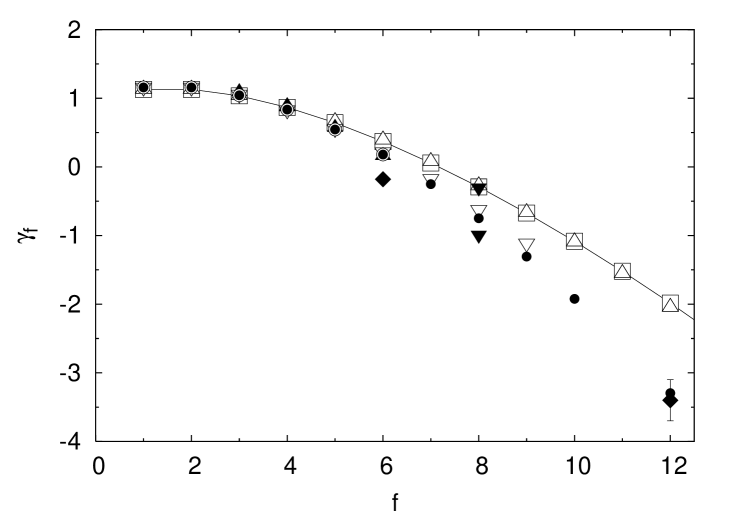
Figure 1: Homogeneous star exponent $\gamma_{f}$ at $d=3$. Open squares: forth order ($\varepsilon^{4}$), open triangles up: third order ($\varepsilon^{3}$), open triangles down [22]: third order RG calculated at fixed dimension ($d=3$). Results of MC simulations are shown by filled symbols, triangles up: [18], triangles down: [19], diamonds: [20], discs: [21].

References

- [1]
- [2] for recent reviews see: C. N. Likos, Phys. Rep. 348 (2001) 267 and in: C. von Ferber, Yu. Holovatch (Eds). Star Polymers, Cond. Matter Phys. 5 (2002) 1-306.
- [3] B. Duplantier, J. Stat. Phys. 54 (1989) 581.
- [4] L. Schäfer, C. von Ferber, U. Lehr, B. Duplantier, Nucl. Phys. B 374 (1992) 473.
- [5] P.-G. de Gennes, Scaling Concepts in Polymer Physics, Cornell University Press, Ithaca and London, 1979. J. des Cloizeaux, G. Jannink, Polymers in Solution, Clarendon Press, Oxford, 1990. L. Schäfer, Excluded Volume Effects in Polymer Solutions, Springer, Berlin, 1999.
- [6] M. E. Cates, T. A. Witten, Phys. Rev. A 35 (1987) 1809.
- [7] C. von Ferber, Yu. Holovatch, Europhys. Lett. 39 (1997) 31; Phys. Rev. E 56 (1997) 6370.
- [8] B. Duplantier, Phys. Rev. Lett. 82 (1999) 880.
- [9] M. Baiesi, E. Carlon, A. L. Stella, Phys. Rev. E 66 (2002) 021804.
- [10] C. von Ferber, Yu. Holovatch, Phys. Rev. E 59 (1999) 6914; Phys. Rev. E 65 (2002) 042801.
- [11] B. Duplantier, A. W. W. Ludwig, Phys. Rev. Lett. 66 (1991) 247.
- [12] see e.g. J. Zinn-Justin, Quantum Field Theory and Critical Phenomena, Clarendon Press, Oxford, 1989. H. Kleinert, V. Schulte-Frohlinde, Critical Properties of -Theories, World Scientific, Singapore, 2001.
- [13] H. Kleinert, J. Neu, V. Schulte-Frohlinde, K. G. Chetyrkin, S. A. Larin, Phys. Lett. B 272 (1991) 39; Phys. Lett. B 319 (1993) 545.
- [14] R. Guida, J. Zinn-Justin, J. Phys. A 31 (1998) 8103.
- [15] V. Schulte-Frohlinde, Yu. Holovatch, C. von Ferber, A. Blumen, to be published.
- [16] V. Schulte-Frohlinde, Yu. Holovatch, C. von Ferber, A. Blumen, Cond. Matter Phys. (2003) submitted.
- [17] L. Schäfer, C. Kappeler, Colloid Polym. Sci. 268 (1990) 995; L. Schäfer, U. Lehr, C. Kappeler, J. Phys. (Paris) I 1 (1991) 211.
- [18] J. Batoulis, K. Kremer, Macromolecules 22 (1989) 4277.
- [19] A. J. Barrett, D. L. Tremain, Macromolecules 20 (1987) 1687.
- [20] K. Ohno, Macromol. Symp. 81 (1994) 121; Cond. Matter Phys. 5 (2002) 15.
- [21] H.-P. Hsu, W. Nadler, P. Grassberger, preprint cond-mat/0310534 (2003).
- [22] C. von Ferber, Yu. Holovatch, Theor. Math. Physics 109 (1996) 1274.