The interplay between screening properties and colloid anisotropy: towards a reliable pair potential for disc-like charged particles

Abstract

The electrostatic potential of a highly charged disc (clay platelet) in an electrolyte is investigated in detail. The corresponding non-linear Poisson-Boltzmann (PB) equation is solved numerically, and we show that the far-field behaviour (relevant for colloidal interactions in dilute suspensions) is exactly that obtained within linearized PB theory, with the surface boundary condition of a uniform potential. The latter linear problem is solved by a new semi-analytical procedure and both the potential amplitude (quantified by an effective charge) and potential anisotropy coincide closely within PB and linearized PB, provided the disc bare charge is high enough. This anisotropy remains at all scales; it is encoded in a function that may vary over several orders of magnitude depending on the azimuthal angle under which the disc is seen. The results allow to construct a pair potential for discs interaction, that is strongly orientation dependent.

I Introduction

Clays, in the generic form of charged platelets, enjoy widespread use in applications ranging from drilling, rheology modification (for paints, cosmetics, cleansers…), catalysis etc. As a significant component of soils, clays are also of importance for crop production. The difficulty of synthesizing clays with well controlled properties (size, composition, charge…) has long hindered their fundamental study. The situation has considerably changed in the last ten years, with the increasing availability of customized synthetic clays, among which Laponite is a prominent example. Yet, our understanding of such systems is rudimentary (see e.g. Mourchid ; Bonn ; Nicolai ; JPCM ; Levitz ; Michot ; Rowan ; Beek and references therein).

A reasonable model for Laponite platelets is that of uniformly charged and infinitely thin discs Rque1 . In this paper, the focus will be on electrostatic interactions between identical charged discs, a crucial ingredient for understanding the phase behaviour and stability of clays in suspensions. The high anisotropy of these objects makes analytical progress difficult. In addition, these discs are typically highly charged, and the electrostatic coupling with their electrolytic environment (microscopic charged species) needs to be described by non-linear theories: the plain linear Debye-Hückel approach should fail. We will work here in the common framework of non-linear Poisson-Boltzmann (PB) theory, where the (dimensionless) electrostatic potential outside the charged macro-ions obeys an equation of the form $\nabla^{2}\phi=\kappa^{2}\sinh\phi$, assuming for simplicity monovalent microions only, the density of which governs the screening length $\kappa^{-1}$ (the Debye length).

In a solution, the typical distance between macroions is often larger than the Debye length (this condition requires a minimal but nevertheless small amount of salt). At these “large” scales, the potential created by a given disc is small enough –compared to thermal agitation– to allow for the linearization of PB equation: $\nabla^{2}\phi\simeq\kappa^{2}\phi$. Accordingly, the potentials within non-linear PB on the one hand, and linearized PB theory with a suitably chosen boundary condition on the other hand, coincide at large enough distance from the colloids, be they of discotic or other shapes. An analytical treatment within linearized PB (LPB) is of course considerably simpler than within PB, but the above remark may be of little practical help if one is not able to derive the relevant boundary condition on the colloid (effective potential), such that the corresponding LPB solution reproduces the PB one in the region of low enough potential. Close to the colloids, non-linear effects prevail (LPB and PB solutions strongly differ), and broadly speaking, microions –essentially counterions– suffer there a high electrostatic coupling and may be considered as “bound”. They decrease the bare charge of the colloid so that its electrostatic signature at large distance defines an effective charge which is usually smaller in absolute value than the bare one (close to the colloid, the effective potential is accordingly smaller than its non-linear counterpart).

For a unique charged sphere in an electrolyte, PB and LPB theories give rise to the same far-field behaviour, of Yukawa type [$\exp(-\kappa r)/r$, where is $r$ is the radial coordinate]; non-linear effects only affect the prefactor (from which the effective charge is defined), preserving the functional form of the potential Belloni ; Hansen ; Levin . The same remark equally applies to an infinite rod. The situation changes, however, for anisotropic objects such as discs or finite size rods Chapot , where non-linear screening phenomena generically affect the functional form of the potential and cannot be subsumed in an effective scalar quantity (effective potential or charge). In other words, whereas the symmetry of the effective colloid clearly remains spherical in the case of spheres, predicting the symmetry of the effective charge distribution and associated electrostatic potential for a highly charged disc is a non trivial question.

It is the purpose of the present work to study how non-linear screening effects and anisotropy conspire to affect the far-field behaviour in the case of discs. It has been shown in Presc that highly charged spheres and infinite rods may be considered as objects of constant effective potential $\phi_{\hbox{\scriptsize eff}}$ (in the sense that $\phi_{\hbox{\scriptsize eff}}$ becomes independent of physico-chemical parameters, provided that $\kappa a>1$ where $a$ is the colloid radius. The complementary results reported here indicate that the constant potential picture goes in fact beyond this analysis, and give the correct symmetry of the effective charge distribution onto the disc. Such a boundary condition (within LPB theory) produces the same electrostatic potential as a highly charged disc within PB. A physical argument allowing to anticipate this correspondence will be presented in section II. Since the exact LPB solution for a disc held at constant potential in an electrolyte is not known, we will introduce in section III a semi-analytical procedure to solve this problem. The characteristic features of the electrostatic potential relevant for clay discs will be obtained, and in order to assess the validity of the constant potential picture, the corresponding electrostatic potential will be compared in section IV to the solutions of the full non-linear PB theory. The latter will be obtained through an iterative numerical procedure. From these results, a pair potential will be constructed for charged discs, that has the same status as the celebrated Derjaguin-Landau-Verwey-Overbeek expression relevant for spheres Belloni ; Hansen ; Levin , and which includes charge renormalization. Concluding remarks will finally be presented in sections V and VI.

II The constant effective potential picture: why?

A disc of radius $a$ and uniform surface charge density $\sigma_{\hbox{\scriptsize bare}}=Z_{\hbox{\scriptsize bare}}\,e/(\pi a^{2})$ is immersed in an infinite sea of electrolyte with bulk density $n_{s}$. From the permittivity $\varepsilon$ of the solvent, the Bjerrum length is defined as $\ell_{B}=e^{2}/(\varepsilon kT)$, where $kT$ is the thermal energy and $e$ denotes the elementary charge. Within non-linear Poisson-Boltzmann theory, the dimensionless potential [$\phi=e\varphi/(kT)$, $\varphi$ being the original electrostatic potential] created by the disc obeys the following equation

$$\nabla^{2}\phi=\kappa^{2}\sinh(\phi)$$ (1)

where $\kappa$ is the inverse Debye length defined through $\kappa^{2}=8\pi\ell_{B}n_{s}$. For convenience, $\phi$ is chosen to vanish at infinity. Eq. (1) holds outside the disc.

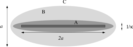
Figure 1: Schematic side view of the charged platelet

Considering a highly charged disc with furthermore $\kappa a>1$, one may partition space into three regions, as sketched in Fig. 1. In region A, the electrostatic coupling between the colloidal disc and the microions is most important and one has $\phi>1$. Outside A, in regions B and C, one has $\phi<1$ and PB equation (1) may be linearized: the corresponding Helmholtz-like LPB equation reads

$$\nabla^{2}\phi=\kappa^{2}\phi.$$ (2)

In addition, in region B, $\phi$ is of unidimensional character and well approximated by the potential created by an infinite charged plane. A contrario, in region C, $\phi$ regains its full 3D nature (2D here with the present azimuthal symmetry). The lateral extension of the “non-linear region” A is given by $\kappa^{-1}$ while $a$ measures the extension of region B. Since we assume $\kappa a>1$, we have A$\,\subset\,$B and moving away from the disc, non-linear effects disappear before the finite size of the disc becomes relevant. In other words, B is the non vanishing intersection between the “linear” region and its one-dimensional counterpart where the solution of Eq. (1) takes the form Andelman

$$\phi_{\text{1\sc D}} = 4\,\hbox{arctanh}\left(\gamma e^{-\kappa z}\right)$$ (3)

$$\simeq 4\gamma e^{-\kappa z}\quad\hbox{in region B.}$$ (4)

In these expressions, $z$ denotes the distance to the plane and, assuming without loss of generality a positive bare charge $\sigma_{\hbox{\scriptsize bare}}$, $\gamma$ is the positive root of the quadratic equation

$$\gamma^{2}-\frac{\kappa e}{\pi\sigma_{\hbox{\tiny bare}}\ell_{B}}\,\gamma+1=0.$$ (5)

In colloidal dispersions, the relevant range for the interactions is that of far-field (except for dense systems) and the behaviour in the non-linear region (A) is of little interest. From Eq. (4), it appears that the potential felt in the linear region B+C, when extrapolated to contact ($z=0$), reads $\phi_{\hbox{\scriptsize eff}}=4\gamma$. As a consequence, solving LPB equation (2) with this boundary condition should provide the same potential outside region A as the PB solution of equation (1).

The above remarks follow from the constraint $a>\kappa^{-1}$ and apply irrespective of the value of the bare charge. In particular, $\sigma_{\hbox{\scriptsize bare}}$ (hence $\phi_{\hbox{\scriptsize eff}}$ through $\gamma$) may be position dependent on the disc. However, we are interested here in highly charged discs for which the non-linear region A exists (for low $\sigma_{\hbox{\scriptsize bare}}$, region A disappears; PB and LPB solutions coincide at all distances and the issue of effective potentials becomes trivial: effective and bare charges are equal). From Eq. (5), it appears that $0<\gamma<1$ and that $\gamma\to 1$ when $\sigma_{\hbox{\scriptsize bare}}$ becomes large, so that $\phi_{\hbox{\scriptsize eff}}\to 4$, and the field created is independent of the bare charge. More details concerning the phenomenon of effective charge saturation may be found in Presc .

We conclude here that a highly charged disc should effectively behave as a constant potential object treated within a linear theory. The corresponding LPB problem will be addressed in the following section but we emphasize before that the argument developed here provides $\phi_{\hbox{\scriptsize eff}}$ to leading order in $\kappa a$. On the basis of the behaviour of charged spheres for which the curvature correction has been computed in JPA [leading to the result $\phi_{\hbox{\scriptsize eff}}=4+2/(1+\kappa a)+{\cal O}(\kappa a)^{-2}$], we anticipate that $\phi_{\hbox{\scriptsize eff}}$ may exceed the threshold 4. A similar behaviour is observed for cylinders of infinite length JPA .

III Semi-analytical solution of the Dirichlet linearized PB problem

III.1 Methodology

If the solution of LPB equation (2) with Dirichlet boundary condition $\phi=\phi_{0}$ was known analytically, the effective charge of highly charged discs Rque2 would follow immediately, enforcing $\phi_{0}=4$ on the disc surface. Unfortunately, such a solution only exists in vacuum (i.e. when $\kappa=0$ Jackson ). To our knowledge, the only solution known at finite $\kappa$ is that associated to Neumann boundary conditions (uniform surface charge) PRE97 . To solve the Dirichlet problem, we have therefore developed a semi-analytical procedure where the problem at hand is recast into a Fredholm integral equation (see below and appendix A).

The general solution of Eq. (2) may be written assuming both cylindrical symmetry around an axis $(Oz)$, and reflection symmetry $z\leftrightarrow-z$:

$$\phi(\rho,z)=\int_{0}^{\infty}A(k)\,J_{0}(k\rho)\,e^{-\sqrt{k^{2}+\kappa^{2}}|z|}\,dk.$$ (6)

In this relation, $(\rho,z)$ denote the cylindrical coordinates and $J_{0}$ is the Bessel function of order 0. The difficulty in the present situation is that the boundary conditions imply that the weight function $A(k)$ obeys the mixed system

$$\int_{0}^{\infty}A(k)\,J_{0}(k\rho)\,dk=\phi_{0}\quad\hbox{for }\rho<a$$ (7)

$$\int_{0}^{\infty}\sqrt{k^{2}+\kappa^{2}}\,A(k)\,J_{0}(k\rho)\,dk=0\quad\hbox{for }\rho>a$$ (8)

where the second equation follows from the vanishing of the normal electric field $\partial_{z}\phi$ on the symmetry plane $z=0$. Starting from Eqs. (7) and (8), the problem is rephrased in terms of an integral equation, solved numerically, from which the function $A(k)$ is computed (see Appendix A). The potential then follows from (6).

III.2 Properties of the solutions

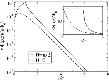
Figure 2: Solution of LPB equation (2) with Dirichlet boundary condition of a uniform potential $\phi=\phi_{0}$ on the disc surface. The quantity $r\phi$ is shown on a linear-log scale to emphasize the far-field behaviour. Here, $\kappa a=2$ and $r=\sqrt{\rho^{2}+z^{2}}$ denotes the distance to the disc center. The continuous curve shows the potential in the direction $\theta=\pi/2$ (as a function of $r/a=\rho/a$), whereas the dashed line shows the behaviour as a function of $r/a=z/a$ along normal axis $\rho=0$ ($\theta=0$). The inset shows $\phi/\phi_{0}$ on a linear scale, again in the two perpendicular directions $\theta=0$ and $\theta=\pi/2$.

A typical solution is shown in Fig. 2. In the remainder, the variable $\theta\in[0,\pi/2]$ denotes the angle between a given direction and the normal to the disc ($\theta=\pi/2$ in the symmetry plane $z=0$ and $\theta=0$ along the normal to the disc, i.e. when $\rho=0$). It may be observed that the potential is anisotropic at all distances, a generic feature of screened electrostatics JPCM ; Chapot : the behaviours for $\theta=0$ and $\theta=\pi/2$ strongly differ, at all scales. The anisotropy of the potential at large scales is encoded in a function $f(\kappa a,\theta)$, such that expression (6) may be written, for $\kappa r\gg 1$,

$$\phi(r,\theta)\,\sim\,Z\,\ell_{B}\,f(\kappa a,\theta)\,\frac{e^{-\kappa r}}{r}\,+\,{\cal O}\left(\frac{e^{-\kappa r}}{r^{2}}\right),$$ (9)

where $r=(\rho^{2}+z^{2})^{1/2}$ again denotes the distance to the disc center. In Eq. (9), the total charge $Z$ of the platelet appears. $Z$ is the integral over the disc surface of the surface charge density $\sigma(\rho)$ [$Ze=\int_{\hbox{\tiny disc}}\sigma({\bf s})d^{2}{\bf s}$]. This density turns out to be related to the anisotropy function through

$$f(\kappa a,\theta)=\int_{\hbox{\scriptsize disc}}\frac{\sigma({\bf s})}{Ze}\,\exp\left(-\kappa\,{\bf\hat{r}}\cdot{\bf s}\right)\,d^{2}{\bf s},$$ (10)

${\bf\hat{r}}$ being a unit vector pointing in the $\theta$ direction. As expected, without electrolyte, $\kappa$ vanishes so that $f=1$ and the potential in (9) takes the familiar form of an isotropic Yukawa expression.

The anisotropy function $f$ and the total charge $Z$, are the key quantities governing far-field behaviour. Note that $Z$ is not known a priori since only the surface potential is imposed. It may be shown that $f$ is related to the weight function $A(k)$ appearing in (6) through

$$\frac{Z\,e}{\varepsilon}f(\kappa a,\theta)\,=\,-i\,\frac{A(i\,\kappa\sin\theta)}{\tan\theta}.$$ (11)

For small arguments, one has $A(x)\propto x$ so that $f(\kappa a,0)=1$, which also means that the total charge is directly accessible through the behaviour along the $\theta=0$ axis :

$$\phi(r,0)\sim Z\,\ell_{B}\,\frac{e^{-\kappa r}}{r}.$$ (12)

Note also that $f(\kappa a,0)=1$ directly follows from (10) since ${\bf\hat{r}}\cdot{\bf s}=0$ when $\theta=0$.

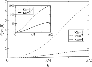
Figure 3: Anisotropy function for $\kappa a$=1, 2 and 4 as a function of azimuthal angle. The inset shows the results on a linear-log scale, for $\kappa a=5$ and $\kappa a=10$.

Figure 3 shows $f(\kappa a,\theta)$ for different salinity conditions. This function increases with $\theta$ and may take large values when $\kappa a$ exceeds a few units (see the inset where the $y$-axis is shown in log scale). On the other hand, for $\kappa a<1$, $f$ remains close to unity in all directions. The potential is strongest in the disc plane ($\theta=\pi/2$), and increasing screening ($\kappa$), one also strongly increases the anisotropy of the electrostatic potential. For a reasonable value $\kappa a=10$, $f(\theta)$ varies by almost 3 orders of magnitude (a factor 930). In figure 4, the complementary information concerning the total charge $Z$ is displayed. This quantity will be further discussed in section III.3. Note that $f(\kappa a,\theta)$ does not depend on $\phi_{0}$, since it probes the repartition of surface charge distribution, not its overall magnitude. On the other hand, $Z$ scales linearly with $\phi_{0}$.

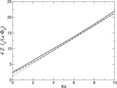
Figure 4: Charge $4Z\ell_{B}/(a\phi_{0})$ as a function of $\kappa a$ (continuous curve). The dashed line shows the result obtained within the simplified two parameter model [Eqs. (15) and (17)-(18), see text]. The dotted line corresponds to Eq. (20).

III.3 An approximate expression for the anisotropy function and charge

It is instructive and useful for practical purposes to have an approximate analytical expression for the function $f(\kappa a,\theta)$. From Eq. (10), that may rewritten

$$f(\kappa a,\theta)\,=\,\frac{2\pi}{Ze}\int_{0}^{a}I_{0}(\kappa\rho\sin\theta)\,\sigma(\rho)\,\rho\,d\rho,$$ (13)

this amounts to look for an approximate expression for the surface charge density $\sigma$. To this aim, we recall Landau that for an ideal conducting disc when $\kappa=0$, $\sigma$ diverges in the vicinity of the edge ($\rho\to a$) since

$$\sigma(\rho)\,=\,\frac{e\,\phi_{0}}{2\pi^{2}a\,\ell_{B}}\,\frac{1}{\sqrt{1-(\rho/a)^{2}}}.$$ (14)

Recall that $\phi_{0}$ denotes the dimensionless electrostatic potential $\phi=\varphi/(\varepsilon kT)$. The singularity of the electric field near sharp edges, which is the reason for the efficiency of lightning conductors, also pertains in presence of an electrolyte. We indeed show in appendix B that when $\kappa\neq 0$, the Dirichlet solution to Eq. (2) exhibits a similar divergence as that present in Eq. (14), namely $\sigma\propto(a-\rho)^{-1/2}$.

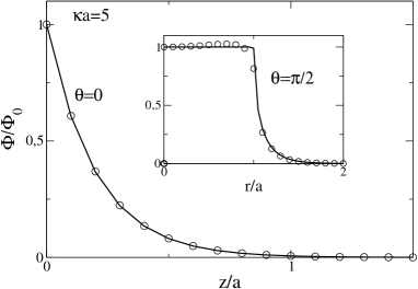
Figure 5: Electrostatic potential following from the two parameters approximation (circles) compared to the exact result (continuous curve, obtained following the method detailed in section III.1 and Appendix A). The main graph corresponds to $\theta=0$ and the inset to $\theta=\pi/2$.

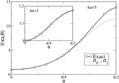
Figure 6: Anisotropy function resulting from the two parameters approximation (15) where $\sigma_{0}$ and $\sigma_{1}$ are determined from (17)-(18), compared to the exact result. The two above parameters are plotted in Fig. 7. Here, $\kappa a=5$ whereas $\kappa a=1$ in the inset.

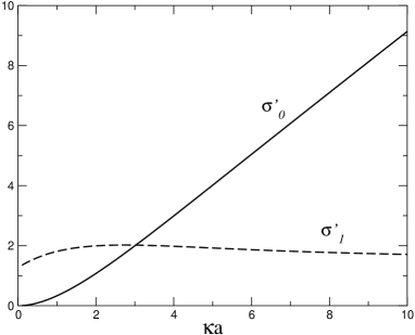
Figure 7: Dimensionless charges $\sigma^{\prime}_{0,1}=2\pi a\ell_{B}\,\sigma_{0,1}/(e\phi_{0})$ following from (15) supplemented with Eqs. (17)-(18), as a function of salinity conditions.

A very simple two parameter ansatz fulfilling this divergence requirement is

$$\sigma(\rho)\,=\,\sigma_{0}+\sigma_{1}\frac{1}{2\,\sqrt{1-(\rho/a)^{2}}}.$$ (15)

From this expression, the anisotropy function may be computed and takes the form

$$f(\kappa a,\theta)\,=\,\frac{\sigma_{0}}{\sigma_{0}+\sigma_{1}}\,\frac{2I_{1}(\kappa a\sin\theta)}{\kappa a\sin\theta}\,+\,\frac{\sigma_{1}}{\sigma_{0}+\sigma_{1}}\,\frac{\sinh(\kappa a\sin\theta)}{\kappa a\sin\theta}$$ (16)

In Eqs. (13) and (16), $I_{0}$ and $I_{1}$ denote modified Bessel functions of the first kind, of order 0 and 1. Expressions (15) and (16) are not exact and there are several ways to choose the two parameters $\sigma_{0}$ and $\sigma_{1}$, that will be determined by two constraints. The simplest possibility is to enforce $\phi(0,0)=\phi(a,0)=\phi_{0}$, but it turned that the choice (hereafter adopted)

$$\phi(0,0)\,=\,\phi_{0}$$ (17)

$$\langle\phi(\rho,0)\rangle\,=\,\phi_{0}$$ (18)

gave better results (the angular brackets denote average over the disc surface). In the limit $\kappa\to 0$, expressions (15) and (16) become exact (with $\sigma_{0}=0$), and we expect that the comparison with exact results at finite $\kappa$ will be all the better as $\kappa a$ is low. It is indeed the case, but when $\kappa a=5$, the approximation is still reasonable (see Figs. 5 and 6). By comparison with the exact solution Fig. 6 shows that the anisotropy of the potential is correctly captured. The corresponding values of partial surface charges $\sigma_{0}$ and $\sigma_{1}$ are shown in Fig. 7, where it may be observed that $\sigma_{0}$ vanishes at low salt, as expected. The associated total charge $Z$ is given by

$$Z\,=\,\frac{\pi a^{2}}{e}\,(\sigma_{0}+\sigma_{1})\,=\,\frac{a\phi_{0}}{2\ell_{B}}\,(\sigma^{\prime}_{0}+\sigma^{\prime}_{1}),$$ (19)

where $\sigma^{\prime}_{1}$ and $\sigma^{\prime}_{2}$ are the quantities plotted in Fig. 7. The charge $Z$ is displayed in Fig. 4, and compares favorably with its exact counterpart. In the above expression, however, $\sigma_{0}$ and $\sigma_{1}$ are functions of $\kappa a$ with unknown analytical expression. As it is desirable to have an analytical formula, we propose the following argument: in the limit of large $\kappa a$, the disc essentially behaves as a an infinite plane, from which we deduce $Z\ell_{B}/a\sim\phi_{0}\kappa a/2$. To estimate the next order correction [constant term $C$ in the expansion $Z\ell_{B}/(a\phi_{0})=(2\kappa a/+C)/4$] we may take the limit $\kappa a=0$ where the solution is given by (14), which imposes $Z\ell_{B}/a=\phi_{0}/\pi$. We therefore obtain

$$Z\,\frac{\ell_{B}}{a}\,\simeq\,\frac{\phi_{0}}{4}\,\left(2\,\kappa a\,+\,\frac{4}{\pi}\right).$$ (20)

Anticipating that the relevant values of $\phi_{0}$ are close to 4 (see sections II and IV), we have factorized the ratio $\phi_{0}/4$ in the previous relation. The quality of approximation (20) is assessed in Figure 4, which shows a good agreement. On the other hand, extracting the correction factor $C$ from the large $\kappa a$ behaviour of the exact $Z$ displayed in Fig. 4 gives $C\simeq 1.88$, to be compared with $C=4/\pi\simeq 1.27$ in Eq. (20).

IV Numerical resolution of the non-linear Poisson-Boltzmann theory

In section III, we have obtained the solution of linearized PB theory with uniform potential boundary condition on the disc. From the discussion developed in section II, we expect the properties described (with $\phi_{0}=4$) to characterize also the far-field created by a highly charged disc, treated within non-linear PB theory. In the following, we critically test this scenario. We first present the numerical procedure used to solve the non-linear PB problem.

IV.1 Green’s function formalism and numerical method

Introducing explictly the charge density $q_{d}({\bf r})$ borne by the disc, Eq. (1) is rewritten

$$\nabla^{2}\phi=\kappa^{2}\sinh(\phi)+4\pi\ell_{B}\,\frac{q_{d}({\bf r})}{e}.$$ (21)

In the subsequent analysis, we will consider the case of a uniformly charged disc for which one has, in cylindrical coordinates

$$q_{d}({\bf r})\,=\,\sigma_{\hbox{\scriptsize bare}}\,\delta(z)\Theta(a-\rho),$$ (22)

where $\Theta$ is the Heaviside step function and $\delta$ the Dirac distribution. However, it is important to emphasize that the results that will be derived are more general, and hold irrespective of the precise PB boundary condition on the disc, provided the bare disc charge is high enough (phenomenon of effective potential saturation).

In view of a numerical resolution, it is convenient to rewrite (21) in the form

$$(\nabla^{2}-\kappa_{0}^{2})\phi\,=\,\kappa^{2}\sinh(\phi)+4\pi\ell_{B}\,q_{d}({\bf r})/e-\kappa_{0}^{2}\phi,$$ (23)

where $\kappa_{0}$ is an arbitrary quantity that will be optimized in order to speed up the resulting procedure (see below). Introducing the Green’s function

$${\cal G}({\bf r},{\bf r}^{\prime})\,=\,-\frac{e^{-\kappa_{0}|{\bf r}-{\bf r}^{\prime}|}}{4\pi|{\bf r}-{\bf r}^{\prime}|},$$ (24)

solution of

$$(\nabla^{2}-\kappa_{0}^{2})\,{\cal G}({\bf r},{\bf r}^{\prime})\,=\,\delta({\bf r}-{\bf r}^{\prime}),$$ (25)

we may recast (23) into

$$\phi({\bf r})=\!\int\!{\cal G}({\bf r},{\bf r}^{\prime})\left[\kappa^{2}\sinh[\phi({\bf r}^{\prime})]+4\pi\ell_{B}\,\frac{q_{d}({\bf r}^{\prime})}{e}-\kappa_{0}^{2}\,\phi\right]d{\bf r}^{\prime}$$ (26)

The contribution arising from $q_{d}$ may be computed analytically:

$$\!\!\!\!\!\!\!\!\!\frac{4\pi l_{B}}{e}\int{\cal G}({\bf r},{\bf r}^{\prime})q_{d}({\bf r}^{\prime})\,d{\bf r}^{\prime}=$$

$$2\frac{Zl_{b}}{a}\int_{0}^{\infty}\,J_{1}(ak)J_{0}(k\rho)\frac{\exp(-|z|\sqrt{k^{2}+\kappa^{2}})}{\sqrt{k^{2}+\kappa^{2}}}dk\,\,$$ (27)

and Eq. (26) is solved iteratively. Starting from the initial guess $\phi_{0}=0$, the right hand side of (26), denoted $\phi_{0}^{\text{out}}$ is computed. This provides a new input potential $\phi_{1}=\alpha\phi_{0}^{\text{out}}+(1-\alpha)\phi_{0}$, which is itself inserted in the rhs of (26) to produce $\phi_{1}^{\text{out}}$ etc. The mixing parameter $\alpha$ is chosen in the range $[10^{-2};10^{-1}]$. Convergence $\phi_{n}\simeq\phi_{n}^{\text{out}}$ is generally achieved for typically 50 to 200 iterations. The procedure may be accelerated starting not from $\phi_{0}=0$ but from the solution of LPB theory [known in the present Neumann case, and given by Eq. (27)]. In addition, it seems that the optimal choice for the numerical screening parameter $\kappa_{0}$ is $\kappa_{0}\simeq\kappa$. We have checked that the solutions found were independent of $\kappa_{0}$ (as they should) by changing this parameter in the range $[\kappa/5;5\kappa]$. The previous procedure bears similarities with the one used in Ref. Raul , where a confined geometry was considered (whereas the situation is that of infinite dilution here).

IV.2 Results

From the method sketched in section IV.1, the numerical solution of the non-linear PB equation (1) may be obtained for arbitrary bare charges and salt content.

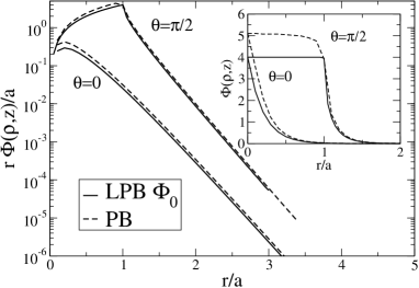
Figure 8: Dashed line: electrostatic potential solution of PB equation (1) for a highly charged disc with uniform bare surface charge (Neumann-like boundary condition, $Z_{\hbox{\scriptsize bare}}\,\ell_{B}/a=60$). Here $\kappa a=5$. The continuous line shows the solution of LPB theory with Dirichlet boundary condition $\phi_{0}=4$ (see section III). The behaviour is shown along the two perpendicular directions $\theta=0$ and $\theta=\pi/2$. The main graph shows $r\phi$ versus $r/a=(\rho^{2}+z^{2})^{1/2}/a$ on a linear-log scale. The inset shows the previous potentials vs $r$ on a linear scale.

To test the constant potential picture put forward in section II (which dwells on the fact that $\kappa a$ is “large enough”) we show in Fig. 8 the PB potential corresponding to a “large” bare charge. It appears that the PB and LPB potential are in excellent agreement except in the immediate vicinity of the disc, so that the constant effective potential prescription seems accurate.

From the PB potentials, we may also extract the effective charge $Z_{\hbox{\scriptsize eff}}$ and anisotropy function $f(\kappa a,\theta)$, that convey a more complete information than a plot like that of Fig. 8. $Z_{\hbox{\scriptsize eff}}$ follows from the far-field behaviour along the $\theta=0$ axis Rque3 [see Eq. (12)]:

$$\phi(r,0)\sim Z_{\hbox{\scriptsize eff}}\,\ell_{B}\,\frac{e^{-\kappa r}}{r}.$$ (28)

Once $Z_{\hbox{\scriptsize eff}}$ is known, $f$ is computed from Eq. (9).

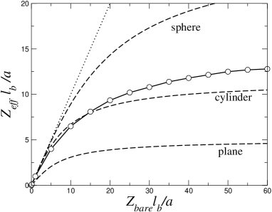
Figure 9: Effective charge as a function of the bare one, for $\kappa a=5$. The circles correspond to the PB solution, and the dotted line has slope one to show the regime of weak coupling where $Z_{\hbox{\scriptsize eff}}=Z_{\hbox{\scriptsize bare}}$. The analytical expressions for a plane, a cylinder and a sphere have also been plotted (see labels).

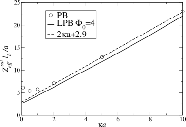
Figure 10: Saturated effective charge $Z_{\hbox{\scriptsize eff}}^{\hbox{\scriptsize sat}}$ as a function of salt (circles). The LPB charge $Z$ is also shown for $\phi_{0}=4$ (continuous line). The dashed line displays the empirical expression (29).

For fixed $\kappa a$, $Z_{\hbox{\scriptsize eff}}$ is a function of the bare charge, see Fig. 9, where the corresponding analytical predictions for planes, spheres and cylinders (of infinite length) have also been reported JPA . Not surprisingly, the behaviour is intermediate between that of infinite planes and spheres, and somehow resembles the results valid for charged cylinders. In addition, $Z_{\hbox{\scriptsize eff}}$ reaches a saturation plateau when $Z_{\hbox{\scriptsize bare}}$ becomes large Presc (see Fig. 9). This asymptotic plateau defines the effective charge at saturation $Z_{\hbox{\scriptsize eff}}^{\hbox{\scriptsize sat}}$, which is shown in Fig. 10. This quantity is an increasing function of salt content (except for $\kappa a<0.5$, see below), since an increase in salt density enhances the macroion/microion screening, which diminishes the amount of “counterion condensation” and consequently increases the effective charge Presc . Figure 10 shows that the constant potential prescription of section II with $\phi_{0}=4$ provides a satisfying description of highly charged platelets, as far as the (effective) charge is concerned. It also appears that the best linear interpolation reads

$$Z_{\hbox{\scriptsize eff}}^{\hbox{\scriptsize sat}}\ell_{B}/a\simeq 2\kappa a+2.9$$ (29)

which is rather close to approximation (20) with the choice $\phi_{0}=4$. It may be observed in Fig. 10 that for low $\kappa a$, the effective charge increases when $\kappa a$ decreases. This aspect will be discussed in section V.2

Computation of anisotropy functions confirms the relevance of the constant effective potential picture (see the comparison proposed in Fig. 11). As shown in the inset, the very high values $f\simeq 900$ predicted from the analysis of section III are indeed found within non-linear PB. Note that the agreement reported in Fig. 11 is only expected at high bare charges. For low bare charges, $f(\kappa a,\theta)$ depends –at variance with its large bare charge counterpart –on the details on the boundary conditions chosen on the disc to solve PB. In the present situation (uniform surface charge), $f$ may be computed analytically with the result JPCM

$$f(\kappa a,\theta)\,=\,2\,\frac{I_{1}(\kappa a\sin\theta)}{\kappa a\sin\theta}.$$ (30)

This functional form is observed from our numerical data, for $Z_{\hbox{\scriptsize bare}}\,\ell_{B}/a<1$ (see Fig. 12). It turns out to differ much from that reported in section III (shown with a dashed line in Fig. 12). We may also observe in Fig. 12 that the “Neumann” expression (30) is lower than the Dirichlet one. The reason is the following : $f$ is sensitive to the charges lying near the edge of the disc [see e.g. Eqs. (10) and (13)]. With Dirichlet boundary condition, the induced surface charge diverges (see appendix B), at variance with the situation of a uniform surface charge, which therefore exhibits a less anisotropic potential. The Dirichlet and Neumann expressions respectively provide upper and lower bounds for the anisotropy function.

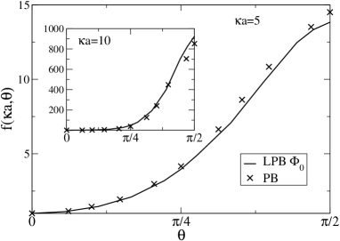
Figure 11: Anisotropy function $f(\kappa a,\theta)$ as a function of azimuthal angle, for $\kappa a=5$. The crosses correspond to the PB result with $Z_{\hbox{\scriptsize bare}}\,\ell_{B}/a=60$ (i.e. in the saturation regime) while the continuous curve shows the constant potential LPB result obtained in section III. Inset: same for $\kappa a=10$.

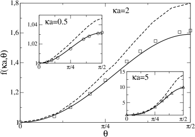
Figure 12: Same as Fig. 11, for a low bare charge $Z_{\hbox{\scriptsize bare}}\,\ell_{B}/a=10^{-2}$. The circles, squares and triangles correspond to $\kappa a=0.5$, 2 and 5. The prediction of Eq. (30) is shown by the continuous line. For the sake of comparison, we also plot with a dashed line the constant potential LPB result already displayed in Fig. 11, which is relevant at high bare charges.

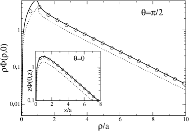
Figure 13: Plot of the PB potential (continuous line) versus distance from disc center in the $\theta=\pi/2$ direction (disc plane). Also displayed are the LPB results for $\phi_{0}=\phi_{0}^{\hbox{\scriptsize opt}}=5.7$ (circles) and for $\phi_{0}=4$ (dotted curve). Here, $\kappa a=0.5$ and $Z_{\hbox{\scriptsize bare}}\ell_{B}/a=15$ corresponding to the saturation plateau (the precise value of $Z_{\hbox{\scriptsize bare}}$ is therefore irrelevant). The inset shows the same quantities along the disc normal.

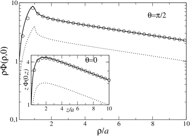
Figure 14: Same as Fig. 13 for $\kappa a=0.1$, with now $\phi_{0}=\phi_{0}^{\hbox{\scriptsize opt}}=9.0$.

In spite of the good agreement shown in Fig. 8, a slight difference may be observed between PB and LPB results. It may be concluded that a value $\phi_{0}$ slightly above 4 may give a better agreement between non-linear and linear profiles. As mentioned at the end of section II, finite $\kappa a$ corrections increase the value of the effective potential above 4 for spherical and rod-like macroions. Figure 13 and 14 show that a similar effect exists for discs : when the $\phi_{0}$ of LPB approach is considered as an adjustable parameter, the agreement between PB and LPB (again for highly charged discs) becomes excellent even at relatively low values of $\kappa a$, such as $\kappa a=0.5$ or even $\kappa a=0.1$. The salt dependence of the above optimal potential, denoted $\phi_{0}^{\hbox{\scriptsize opt}}$, is shown in Fig. 15. One observes that $\phi_{0}^{\hbox{\scriptsize opt}}$ is close to 4 for $\kappa a>5$, but may take significantly different values at lower $\kappa a$. This leads to reconsider the plot of Fig. 10 since the (relative) discrepancy PB/LPB may arise from discarding finite $\kappa a$ effects (i.e. enforcing $\phi_{0}=4$). Fig. 16 compares PB saturated effective charge to its LPB counterpart, with $\phi_{0}=\phi_{0}^{\hbox{\scriptsize opt}}$. Both quantities now agree very well. This latter comparison is a severe and successful test for the relevance of the constant potential prescription.

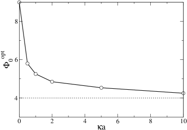
Figure 15: Circles: Values of the optimal surface potential $\phi_{0}^{\hbox{\scriptsize opt}}$ to be imposed within LPB theory to produce the same far-field behaviour as a highly charged disc treated within PB (saturation limit). The dashed line indicates the high salt limiting behaviour $\phi_{0}=4$.

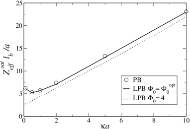
Figure 16: Same as Fig. 10 but with $\phi_{0}=\phi_{0}^{\hbox{\scriptsize opt}}$ (the latter quantity being plotted in Fig. 15) instead of $\phi_{0}=4$. For completeness, the results obtained with $\phi_{0}=4$ are shown by the dotted line.

V Discussion

V.1 Pair potential

From the properties of the one body electrostatic potential $\phi$ discussed previously, one may obtain the large distance behaviour for the pair potential $U_{12}$ in the situation of two discs (radii $a_{1}$ and $a_{2}$) in an electrolyte

$$U_{12}\,=\,Z_{\hbox{\scriptsize eff,1}}\,Z_{\hbox{\scriptsize eff,2}}\,\,\ell_{B}\,f(\kappa\,a_{1},\theta_{1})\,f(\kappa\,a_{2},\theta_{2})\,\,\frac{e^{-\kappa r}}{r}.$$ (31)

Here $\theta_{i}$ is the angle between the normal to disc $i$ and the center-to-center direction ${\bf r}_{12}$ (with $|{\bf r}_{12}|=r$). The validity of such an expression at intermediate or short distances (i.e. $\kappa r$ of order 1) is unclear, since polarization effects of disc $i$ on disc $j$ should at least perturb the symmetry of the effective charge distribution, and hence alter the one body expression for $f$ plotted in Fig. 11. We also note that the sub-leading terms in Eq. (31) that become more important as $\kappa r$ decreases, involve a more complex dependence on relative orientations (with all Euler angles becoming relevant, contrary to the far-field case where only $\theta_{1}$ and $\theta_{2}$ matter).

We may conclude here that at fixed center-to-center distance $r$, the favored configuration is that where the discs are parallel and perpendicular to their center-to-center vector ${\bf r}_{12}$. The T-shape configuration is intermediate and the most repulsive one corresponds to coplanar discs (parallel to ${\bf r}_{12}$, as coins lying on a table). However, the situation changes if one fixes the closest distance $\cal D$ between the two discs. Comparing the configuration $\theta_{1}=\theta_{2}=\pi/2$ where ${\cal D}=r-a_{1}-a_{2}$ to that with $\theta_{1}=\theta_{2}=0$ for which ${\cal D}=r$ requires to compare $\cal Q$ defined as

$${\cal Q}\,=\,f\left(\kappa\,a_{1},\frac{\pi}{2}\right)\,f\left(\kappa\,a_{2},\frac{\pi}{2}\right)\,\,e^{-\kappa(a_{1}+a_{2})}$$ (32)

with 1. From approximate expression (30), it appears that $\cal Q$ is always smaller than 1. Instead of (30), a more reliable expression for the anisotropy is provided by (16), which leads to the same conclusion. We therefore recover the intuitive result that the less repulsive configuration at fixed $\cal D$ is for $\theta_{1}=\theta_{2}=\pi/2$ (two coins on a table).

V.2 Behaviour at low $\kappa a$

In the present study, we have focused on the regime $\kappa a>1$ since according to the argument of section II, it corresponds to the situation where the effective potential may be predicted analytically. It appears that the Debye length acts as a local probe to reveal the anisotropy of the macroion under study. Hence, in the limit of small $\kappa a$ where this probe cannot resolve the disc dimension, we found that the anisotropy disappears: $f(\kappa a=0,\theta)=1,~{}\forall\,\theta$. We may then speculate that at small $\kappa a$, the precise form of the macroion becomes irrelevant so that we should recover the same results as for spheres Rque5 . From the analysis of Ramanathan Ramanathan , we may consequently expect in the saturation regime :

$$Z_{\hbox{\scriptsize eff}}^{\hbox{\scriptsize sat}}\,\frac{\ell_{B}}{a}~{}\stackrel{{\scriptstyle\kappa a\ll 1}}{{\sim}}~{}-2\ln(\kappa a)+2\ln[-\ln(\kappa a)]+4\ln 2$$ (33)

Such an expression diverges for $\kappa a\to 0$, indicating that potential (or charge) renormalization ultimately becomes irrelevant. However, with the lowest value of $\kappa a$ investigated in this work ($\kappa a=0.1$), we have measured $Z_{\hbox{\scriptsize eff}}^{\hbox{\scriptsize sat}}\simeq 6.1\,a/\ell_{B}$ (see Fig. 10), whereas Eq. (33) gives approximately a value 6.7. Whether this agreement is incidental or not is unclear. We also note that if the discs behave as spheres for very low $\kappa a$, their saturated effective potential should coincide with $Z_{\hbox{\scriptsize eff}}^{\hbox{\scriptsize sat}}\,\ell_{B}/a$. This is not the case for $\kappa a=0.1$ where we measured $\phi_{0}^{\hbox{\scriptsize opt}}\simeq 9$. This may indicate what a salinity condition $\kappa a=1/10$ is not low enough to enter the “spherical” regime.

V.3 Validity of the PB approach

We now discuss the validity of the Poisson-Boltzmann theory underlying the present analysis. Such an approach neglects microionic correlations (be they of electrostatic or other origin, such as excluded volume) while macroion/microion electrostatic correlations are correctly incorporated. In the vicinity of the charged discs where the counterion density may become large, the neglected correlations are most important, and may invalidate PB theory if the disc bare charge is too large (say $Z_{\hbox{\scriptsize bare}}>Z_{\hbox{\scriptsize bare}}^{\hbox{\scriptsize corr}}$). Since we have considered here the situation of high $Z_{\hbox{\scriptsize bare}}$ to explore the PB saturation plateau, we need to justify the relevance of such a plateau. In other words, this amounts to elucidating the circumstances under which $Z_{\hbox{\scriptsize sat}}<Z_{\hbox{\scriptsize bare}}^{\hbox{\scriptsize corr}}$, since for $Z_{\hbox{\scriptsize bare}}>Z_{\hbox{\scriptsize sat}}$, one has, roughly speaking, $Z_{\hbox{\scriptsize eff}}\simeq Z_{\hbox{\scriptsize sat}}$.

For a salt-free system, Netz has considered the validity of PB theory in planar, cylindrical and spherical geometries Netz . Since no general result exists, we present here a a simple argument concerning discs, which goes as follows (see Levin for the spherical case). Microionic correlations may be accounted for by the coupling parameter $\Gamma=\ell_{B}/d$ where $d$ is a typical distance between microions in the double-layer. This distance is bounded from below by that, denoted $d^{*}$, where all $Z$ monovalent counterions are artificially condensed onto the disc (as would happen in the low temperature limit). It may be estimated writing that the typical surface per microion $(d^{*})^{2}$ on the disc is the mean value $\pi a^{2}/Z$. Hence,

$$\Gamma\,\simeq\,\sqrt{\ell_{B}^{2}\,\sigma_{\hbox{\scriptsize bare}}}\simeq\sqrt{Z_{\hbox{\scriptsize bare}}\,\ell_{B}^{2}/(\pi a^{2})}.$$ (34)

For microions with valency $z$, one would obtain

$$\Gamma\simeq\sqrt{z^{3}\,Z_{\hbox{\scriptsize bare}}\,\ell_{B}^{2}/(\pi a^{2})}.$$ (35)

For the sake of the argument, the factor $\pi$ could be omitted. The important point here is that $Z_{\hbox{\scriptsize bare}}\,\ell_{B}/a$ may be large, which corresponds to the saturation regime of PB theory, with still $\Gamma<1$, which justifies the mean-field assumption underlying PB. With typical Laponite parameters Rque1 and monovalent microions, we have $\Gamma\simeq 0.7$ for $Z_{\hbox{\scriptsize bare}}\simeq 700$, a reasonable value for the charge. In addition, $Z_{\hbox{\scriptsize bare}}\,\ell_{B}/a\simeq 33$ which is well beyond the linear regime where effective and bare parameters coincide (see Fig. 9, or Fig. 17 corresponding to a lower salt concentration for which $Z_{\hbox{\scriptsize bare}}\,\ell_{B}/a\simeq 33$ lies in the saturated region). We finally note that the intersection between the PB saturation regime and the consistency condition $\Gamma<1$ is all the larger as $a/\ell_{B}$ is big Groot . But of course, when $Z_{\hbox{\scriptsize bare}}$ strictly diverges, $\Gamma$ exceeds a few units and PB breaks down. Finally, to be specific, $Z_{\hbox{\scriptsize bare}}^{\hbox{\scriptsize corr}}$ would be defined as the value of $Z_{\hbox{\scriptsize bare}}$ such that the coupling parameter $\Gamma$ is of order unity. The case of Laponite seems somehow borderline, since $Z_{\hbox{\scriptsize bare}}$ does not differ much from $Z_{\hbox{\scriptsize bare}}^{\hbox{\scriptsize corr}}$ (on the order of a few thousands).

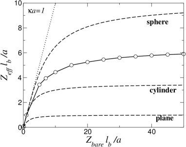
Figure 17: Same as Fig. 9 with $\kappa a=1$.

V.4 The case of asymmetric electrolytes

Bearing in mind the classical rule that increasing the valency of microions decreases the range of validity of PB theory [see Eq. (35)], we may extend previous results to 1:2 and 2:1 electrolytes. The key ingredient in the constant effective potential prescription is indeed the analytical solution of the planar (1D) PB equation. The latter problem has been solved by Gouy almost a century ago Gouy , and it turns out that the counterpart of the monovalent result $\phi_{0}=4$ reads $\phi_{0}\,=\,6$ for 2:1 electrolytes (i.e monovalent counterions and divalent coions, or more precisely when the ratio of coion to counterion valency equals 2). In the reverse 1:2 situation, we have

$$\phi_{0}\,=\,6(2-\sqrt{3})\simeq 1.608.$$ (36)

The 1:2 effective potential is smaller that the 2:1 potential since screening by monovalent counterions is less efficient than with divalent ones (hence a higher effective potential, and a higher effective charge Tellez ).

By simply plugging the above expressions for $\phi_{0}$ into the expressions derived in the previous sections for symmetric electrolytes, one may describe 1:2 and 2:1 situations as well. We finally note that the electrolyte asymmetry does not affect the anisotropy function $f(\kappa a,\theta)$: LPB equation takes the same form (modulo a change in the numerical value of $\kappa$) and only $\phi_{0}$ is affected.

V.5 Comparison with existing results

In Ref JPCM , we have addressed a similar issue as in the present paper. However, neither the LPB at constant potential nor the PB theory were solved. The anisotropy function has been estimated there from the Neumann LPB result with a uniform surface charge. This leads to expression (30), which has been shown in Figure 12 be an underestimation of the Dirichlet result [and the agreement between PB and Eq. (30) is simply due to the low charge in Fig. 12, see Fig. 11].

Following similar lines, the saturated effective charge of discs have been estimated in JPCM from the Neumann LPB solution. When the resulting dimensionless potential is equated to 4 on the disc center, we obtain JPCM

$$Z_{\hbox{\scriptsize eff}}^{\hbox{\scriptsize sat}}\,=\,\frac{a}{\ell_{B}}\,\frac{2\,\kappa a}{1-\exp(-\kappa a)},$$ (37)

which is very close to $2\kappa a$ as soon as $\kappa a>2$. Such an expression only captures the leading order behaviour (the planar limit), but misses the offset correction (2.9) as appears in Eq. (29).

VI Conclusion

We have presented in this paper a detailed comparison between the electrostatic potentials obtained within Poisson-Boltzmann (PB) and Linearized PB approximations, for a charged disc in an electrolyte. We have proposed a new and efficient semi-analytical method to solve the LPB problem at constant surface potential $\phi_{0}$. The procedure used is not restricted to the specific problem considered here, and allows to solve more general situations of the form given by Eq. (40). On the other hand, the PB problem has been solved numerically following similar lines as in Ref Raul . We have shown that the far-field potential created by a highly charged disc within PB is remarkably close to its LPB counterpart with a suitably chosen value of $\phi_{0}$, which therefore defines the effective potential of the charged discs. As expected from the argument put forward in section II, the latter quantity is close to 4 (meaning that the effective surface potential is close to $4kT/e$) whenever $\kappa a$ is larger than a few units, say $\kappa a>3$. These results extend the conclusion of Ref. Presc . The argument of section II should in fact apply for any charged macro-ion for which the curvature is smaller than the inverse Debye length $\kappa$ of the surrounding electrolyte. Note also that in the limit of high bare charge, the details of the bare charge distribution onto the discs are irrelevant. In this respect, the results obtained here within PB with uniform surface charge are generic and would resist to charge modulation.

The scenario emerging is that due to non-linear screening phenomena, highly charged macroions may be considered as effective objects with a uniform surface potential and can be treated within a linear theory (provided short distance features are irrelevant) which considerably simplifies the analysis and opens simulation routes. In addition, this potential is constant provided there is enough salt in the solution, in the sense that it no longer depends on physico-chemical parameters. Such a viewpoint not only predicts satisfactorily their effective charge, but also reproduces accurately the anisotropy of their potential. The latter property, embodied in the function $f(\kappa a,\theta)$ is a key feature of screened electrostatic interactions and may have non negligible –and hitherto largely unexplored– consequences. It is responsible for the rich phase behaviour and orientational ordering of colloidal molecular crystals PRL . Its effects on the phase behaviour of clays, especially at moderately to high salt concentrations where large energy barriers $f(\theta=\pi/2)-f(\theta=0)$ are observed, will be the subject of future work.

The authors acknowledge fruitful discussions with J.J. Weis, B. Jancovici, F. van Wijland, M. Aubouy and H. Lekkerkerker.

Appendix A

Mixed boundary value problems are rather frequent in electrostatics but also in diffusion and elasticity problems Lowengrub ; Collins (conduction of heat, diffusion of thermal neutrons, punch or crack problems etc.). They may be encountered in hydrodynamics as well Lamb . They generally arise whenever a potential is prescribed over part of a boundary whereas its normal derivative is specified over the complementary part. The theory of dual integral equations turns out to be a powerful tool for such situations. In this appendix, we give more details about the problem of finding the solution $A(k)$ to equations (7) and (8). To begin with, it is convenient to recast them in the form

$$\left\{\begin{array}[]{lcrr}\displaystyle\int_{0}^{\infty}\frac{\displaystyle g(u)}{\sqrt{u^{2}+(\kappa a)^{2}}}\,J_{0}(xu)\,du&=&1&\quad\hbox{for}\,\,x<1\\ \displaystyle\int_{0}^{\infty}g(u)\,J_{0}(xu)\,du&=&0&\quad\hbox{for}\,\,x>1\end{array}\right.$$ (38)

where dimensionless quantities have been introduced: $u=k\,a$, $x=\rho/a$ and $g(u)=\sqrt{u^{2}+(\kappa a)^{2}}\,A(u)/\Phi_{0}$. Solutions of the previous equations for $\kappa=0$ (no salt case) have been derived by Titchmarsh Titchmarsh . The procedure, based on rephrasing the dual integral equations by means of some invertible linear operators gives the solution

$$A_{\kappa=0}(u)\,=\,\frac{2\Phi_{0}}{\pi}\,\frac{\sin u}{u}$$ (39)

and the corresponding potential is that which leads to equation (14) for the charge. A generalization of Titchmarsh’s method has been proposed by Sneddon Sneddon for dual integral equations of the type

$$\left\{\begin{array}[]{lcrr}\displaystyle\int_{0}^{\infty}u^{-2\alpha}\,(1+\omega(u))\,g(u)\,J_{\nu}(xu)\,du&=&1&\quad\hbox{for}\,\,x<1\\ \displaystyle\int_{0}^{\infty}g(u)J_{\nu}(xu)\,du&=&0&\quad\hbox{ for}\,\,x>1\end{array}\right.$$ (40)

where $\omega$ is an arbitrary function. Equations (40) and (38) can be made equivalent by taking

$$\omega(u)\,=\,\frac{u}{\sqrt{u^{2}+(\kappa a)^{2}}}-1$$ (41)

with $\alpha=1/2$ and $\nu=0$ (for $\omega(u)=0$, we recover the no salt case). The problem at hand –that fits into the general framework of Sneddon – may be reduced to that of solving a Fredholm equation of the second kind. Following Sneddon, we write equations (40) in the form:

$$\begin{array}[]{lcl}\hbox{S}_{-\frac{1}{2},1}[(1+\omega(u))g(u)/u,x]&=&2/x\quad\hbox{for}\,\,x<1\\ \hbox{S}_{0,0}[g(u)/u,x]&=&0\quad\hbox{ for}\,\,x>1\end{array}$$ (42)

where $\hbox{S}_{\alpha,\beta}$ is the modified Hankel operator defined by:

$$\hbox{S}_{\alpha,\beta}[\lambda(u),x] \equiv \hbox{S}_{\alpha,\beta}\lambda(x)$$

$$= 2^{\beta}\,x^{-\beta}\,\int_{0}^{\infty}u^{-\beta}\,\lambda(u)\,\hbox{J}_{2\alpha+\beta}(xu)\,du$$

We then introduce the function $h$ through

$$g(u)\,=\,u\,S_{0,\frac{1}{2}}h(u).$$ (43)

This function $h(u)$ is the central object in the present procedure. After some cumbersome algebra based on the properties of the modified Hankel operators (for details, see Sneddon ), we find that the function $h_{2}=u\,h(u)$ defined on $[1;\infty]$ vanishes while its counterpart $h_{1}$ defined on $[0;1]$ is the solution of the following Fredholm equation of the second kind:

$$h_{1}(x)+\int_{0}^{1}h_{1}(u)K(x,u)du\,=\,2/\sqrt{\pi}.$$ (44)

The kernel $K(x,u)$ is defined in the whole $xu$-plane by:

$$K(x,u)\,=\,\sqrt{\frac{\pi}{2}}\kappa a(I_{1}(\kappa a|x-u|)-L_{1}(\kappa a(x+u)))$$ (45)

and $I_{1}$ and $L_{1}$ denote respectively the modified Bessel function and Struve function of the first kind, of order one. The weight function $g(u)$ appearing in equation (38) is recovered by means of the integral:

$$g(u) = \sqrt{u^{2}+(\kappa a)^{2}}\,A(u)/\Phi_{0}$$ (46)

$$= \frac{u}{\sqrt{\pi}}\,\int_{0}^{1}\cos{(ut)}\,h_{1}(t)\,dt.$$ (47)

The potential finally follows from equation (6). The Fredholm equation (44) is solved numerically by an iterative procedure, starting by an constant initial guess for $h_{1}$.

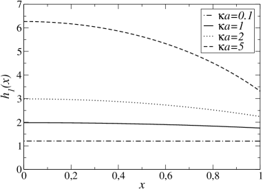
Figure 18: Plots of $h_{1}(x)$ [solution of the integral equation (44)] versus rescaled distance $x$ for different values of $\kappa a$. For $\kappa a=0.1$, $h_{1}$ is very close to its no salt limit $2/\sqrt{\pi}\simeq 1.13$.

In the limit $\kappa=0$, $K(x,u)=0$ so that, from Eq. (44), $h_{1}=2/\sqrt{\pi}$. The function $g(u)$ in (47) follows immediately: $g(u)\,=\,(2/\pi)\sin u$, which is fully consistent with (39). Finally note that the functions $h_{1}(x)$, plotted in Fig. 18 for different values of $\kappa a$, are related to the surface charge density of the disk $\sigma(x)$ through the equation:

$$\sigma(x)\,=\,\frac{h_{1}(x)}{\sqrt{\pi}\,\sqrt{1-x^{2}}}.$$ (48)

The function $h_{1}$ can be well approximated by a quadratic polynomial. The corresponding charge $\sigma(x)$ may then be used to compute analytically approximated effective charges, anisotropy functions and weigh functions $A(u)$. This procedure is an alternative to the ansatz proposed in equation (15), the latter being more suited for an analytical treatment. We finally note that from Eq. (48) and the regular behaviour of $h_{1}$ observed on Fig. 18 for $x\to 1$, the surface charge diverges near the edge of the disc like $(1-x)^{-1/2}$, see appendix B.

Appendix B

We show here that the LPB surface charge distribution $\sigma(\rho)$ –arising from the condition of constant surface potential on the disc– exhibits in an electrolyte the same edge effect as in vacuum, where it diverges as $(a-\rho)^{-1/2}$ when $\rho\to a^{-}$ Landau .

Figure 19: The wedge geometry. The conductor is represented as the shadowed part and its boundaries by the thick line.

We consider the more general problem of a wedged-shape conductor with angle $\beta$ (see Fig. 19). The imposed potential is denoted $\phi_{0}$. Being interested in the behaviour near the sharp edge where the situation is of cylindrical symmetry, we introduce the cylindrical coordinates ($r$, $\psi$) in a plane perpendicular to the apex of the wedge. With rescaled distance $\widetilde{r}=\kappa r$, we look for solutions of LPB equation (2)

$$\widetilde{r}\,\frac{\partial}{\partial\widetilde{r}}\left(\widetilde{r}\,\frac{\partial\phi}{\partial\widetilde{r}}\right)\,+\,\frac{\partial^{2}\phi}{\partial\psi^{2}}\,=\,\widetilde{r}^{2}\phi$$ (49)

in a form with separated variables

$$\phi(\widetilde{r},\psi)\,=\,R(\widetilde{r})\,\Psi(\psi).$$ (50)

With the boundary condition $\phi(\widetilde{r},\psi=0)=\phi(\widetilde{r},\psi=\beta)=\phi_{0}$ for all $\widetilde{r}$ in the vicinity of the wedge (i.e. $\widetilde{r}$ close to 0), the solution reads:

$$R(\widetilde{r})=A_{\nu}I_{\nu}(\widetilde{r})$$ (51)

$$\Psi(\psi)=\alpha_{\nu}\sin(\nu\psi).$$ (52)

Here, $\nu=n\pi/\beta$ where $n\in\mathbb{N}$; $A_{\nu}$ and $\alpha_{\nu}$ are arbitrary constants. In the vicinity of the wedge, the potential therefore takes the form

$$\phi(\widetilde{r},\psi)\,=\,\phi_{0}\,+\,\sum_{n=1}^{\infty}A_{n}\sin\left(\frac{n\pi\psi}{\beta}\right)\,I_{n\pi/\beta}(\widetilde{r}).$$ (53)

The dominant term when $\widetilde{r}\to 0$ corresponds to $n=1$, and scales like $\widetilde{r}^{\,\pi/\beta}$. The associated surface charge behaves like $\sigma(\widetilde{r})\propto\widetilde{r}^{\,\pi/\beta-1}$, hence like $\widetilde{r}^{\,-1/2}$ near the edge of a disc $(\beta=2\pi)$. This result has been used to choose the functional form (15).

References

- (1) A. Mourchid, A. Delville, J. Lambard, E. Lécolier, and P. Levitz, Langmuir 11, 1942 (1995); A. Mourchid, E. Lécolier, H. van Damme and P. Levitz, Langmuir 14, 4718 (1998).
- (2) D. Bonn, H. Kellay, H. Tanaka, G. Wegdam and J. Meunier, Langmuir 15, 7534 (1999).
- (3) T. Nicolai and S. Coccard, J. Colloid Interface Sci. 244, 51 (2001).
- (4) E. Trizac, L. Bocquet, R. Agra, J.-J. Weis and M. Aubouy, J. Phys.: Condens. Matt. 14, 9339 (2002).
- (5) F. Cousin, V. Cabuil and P. Levitz, Langmuir 18, 1466 (2002).
- (6) L.J. Michot, J. Ghanbaja, V. Tirtaatmadja and P.J. Scales, Langmuir 17, 2100 (2001).
- (7) D. Rowan and J.-P. Hansen, Langmuir 18, 2063 (2002).
- (8) D. van der Beek and H.N.W. Lekkerkerker, Europhys. Lett. 61, 702 (2003).
- (9) These colloidal discs bear a negative bare charge. They have a radius of approximately 15 nm and a thickness smaller than 1nm, see e.g. Laponite technical report, Southern Clay Products Inc., Laporte plc. The results reported here correspond to a positive bare charge. They immediately transpose to the Laponite case by a change of sign.
- (10) L. Belloni, Colloids and Surfaces A: Physicochem. Eng. Aspects 140, 227 (1998); J. Phys.: Condens. Matter 12, R549 (2000).
- (11) J.-P. Hansen and H. Löwen, Annu. Rev. Phys. Chem. 51, 209 (2000).
- (12) Y. Levin, Rep. Prog. Phys. 65, 1577 (2002).
- (13) D. Chapot, L. Bocquet and E. Trizac, J. Chem. Phys 120, 3969 (2004).
- (14) E. Trizac, L. Bocquet and M. Aubouy, Phys. Rev. Lett. 89, 248301 (2002); L. Bocquet, E. Trizac and M. Aubouy, J. Chem. Phys. 117, 8138 (2002).
- (15) D. Andelman in Membranes, their Structure and Conformation, edited by R. Lipowsky and E. Sackmann (Elsevier, Amsterdam 1996).
- (16) M. Aubouy, E. Trizac and L. Bocquet, J. Phys. A: Math. Gen. 36, 5835 (2003).
- (17) From Eq. (5), highly charged means in practice .
- (18) J.D. Jackson, Classical Electrodynamics, John Wiley & Sons, New-York, (1975).
- (19) E. Trizac and J.P. Hansen, Physical Review E 56, 3137 (1997).
- (20) L.D. Landau and E.M. Lifschitz, Electrodynamics of continuous media (Pergamon Press, Oxford, 1984).
- (21) R.J.F. Leote de Carvalho, E. Trizac and J.-P. Hansen, Europhys. Lett. 43, 369 (1998).
- (22) The existence of a given direction along which the effective charge may be directly measured is a specific feature of macroions with vanishing internal volume. In general, as happens for a disc of finite thickness, the anisotropy function differs from unity in all directions. It is consequently more difficult –and to some extent arbitrary– to disentangle effective charge effects from those due to anisotropy.
- (23) We are interested here again in the far-field behaviour. For (no electrolyte), a disc and a sphere behave identically, as a usual monopole.
- (24) G.V. Ramanathan, J. Chem. Phys. 88, 3887 (1988).
- (25) R.R. Netz, Eur. Phys. J. E 5, 557 (2001); Eur. Phys. J. E 13, 43 (2004).
- (26) A similar conclusion is reached in R.D. Groot, J. Chem. Phys. 95, 9191 (1991).
- (27) G.L. Gouy, J. Phys. 9, 457 (1910).
- (28) G. Téllez and E. Trizac, Phys. Rev. E (2004), in press.
- (29) R. Agra, F. van Wijland and E. Trizac, Phys. Rev. Lett. 93, 018304 (2004).
- (30) W.D. Collins, Mathematika, 6, 120-133 (1959).
- (31) I.N. Sneddon and M. Lowengrub, Crack problems in the classical theory of elasticity, John Wiley, NY, 1969.
- (32) H. Lamb, Hydrodynamics, 6th ed., Cambridge University Press, 1932.
- (33) E.C. Titchmarsh, Introduction to the theory of Fourier integrals, 2nd ed., Clarendon Press, Oxford (1948).
- (34) I.N. Sneddon, Mixed boundary value problems in potential theory, North Holland, 1966.