Dynamics of a trapped ultracold two-dimensional atomic gas

Dynamique d’un gaz d’atomes ultra froid piégé à deux dimensions

Abstract

This article is devoted to the study of two-dimensional Bose gases harmonically confined. We first summarize their equilibrium properties. For such a gas above the critical temperature, we also derive the frequencies and the damping of the collective oscillations and we investigate its expansion after releasing of the trap. The method is well suited to study the collisional effects taking place in the system and in particular to discuss the crossover between the hydrodynamic and the collisionless regimes. We establish the link between the relaxation times relevant for the damping of the collective oscillations and for the time-of-flight expansion. We also evaluate the collision rate and its relationship with the relaxation time.

Mots-clés : Gaz en basse dimension ; Oscillations collectives ;Temps de vol

Version française abrégée

Cet article est consacré l’étude des gaz de Bose à deux dimensions en présence d’un confinement harmonique. Nous abordons tout d’abord les propriétés d’équilibre de ce système. Nous dérivons ensuite, au-dessus de la température critique, l’expression des fréquences et de l’amortissement des modes collectifs de basse énergie et nous étudions avec le même formalisme l’évolution du nuage d’atomes lorsque le confinement est brutalement supprimé. La méthode utilisée permet de décrire le gaz dans tous les régimes collisionels, du régime sans collision au régime hydrodynamique. Nous établissons le lien entre les temps de relaxation qui décrivent les modes d’oscillation et l’expansion du nuage après coupure du piège. Nous évaluons également l’expression du taux de collision et sa relation avec le taux de relaxation des modes de basse énergie.

1 Introduction

Quantum gases in reduced dimensionality are now experimentally available. Two-dimensional Bose gases have been realized by trapping atomic hydrogen at the surface of liquid helium [1, 2]. Such a gas, confined into a box, undergoes at sufficiently low temperature a superfluid transition known to be of the Berezinskii-Kosterlitz-Thouless type [3, 4, 5].

Recently, a few experiments with laser-cooled atoms have approached the two-dimensional regime. The method used consists in realizing very anisotropic confinement in such a way that one degree of freedom is frozen to zero motion oscillations. The crossover to two-dimensions occurs when the thermal energy is below the vibrational energy in the tightly confined direction. Such a regime has been reached in standing-wave dipole traps [6]. Alternatively, an elliptically focused laser beam has been fed by a Bose-Einstein condensate leading to a two-dimensional configuration [7]. Evaporative cooling of an atomic gas has also been performed at the crossover to two dimensions in an optical surface trap [8]. A two-dimensional Bose-Einstein condensate has been achieved with ultracold cesium atoms trapped in a gravito-optical surface trap [9]. Notice that two-dimensional trapping by means of a field-induced adiabatic potential has been recently proposed [10] and realized experimentally in the group of H. Perrin and V. Lorent [11]. In all those systems the two-dimensional confinement can be considered as harmonic.

The harmonic confinement introduces very different features from the physics one would obtain in a box. As explained below, for an ideal Bose gas, Bose-Einstein condensation occurs at finite temperature in the presence of a harmonic potential in contrast to the homogeneous case [12].

The paper is devoted to the physics of two-dimensional Bose gases harmonically trapped above the critical temperature. First, we discuss the thermodynamic properties and the shift of the critical temperature of an ideal gas at fixed number of particles due to the finite size of the sample. We discuss briefly the role of interactions. Second, we study the dynamics of the gas through low-lying collective modes and time of flight expansion by including dissipative and mean-field effects.

2 Thermodynamical properties

2.1 Ideal gas

We consider $N$ bosons confined by a two-dimensional harmonic trap of angular frequencies $\omega_{x}$ and $\omega_{y}$. By contrast with a non-confined Bose gas, Bose-Einstein condensation is expected to occur since the number of atoms in the excited states saturates to an upper value $N^{\prime}_{\rm max}$:

$$N^{\prime}_{\rm max}=\sum_{(n_{x},n_{y})\neq(0,0)}\frac{1}{\exp[\hbar(n_{x}\omega_{x}+n_{y}\omega_{y})/(k_{B}T)]-1}\simeq\frac{\pi^{2}}{6}\frac{k_{B}T}{\hbar\omega_{x}}\frac{k_{B}T}{\hbar\omega_{y}}.$$ (1)

The critical temperature for an ideal Bose-Einstein condensation $T_{c}^{0}$ is readily obtained from this formula by setting $N^{\prime}_{\rm max}=N$:

$$k_{B}T_{c}^{0}=\frac{\hbar\bar{\omega}\sqrt{6N}}{\pi},$$ (2)

with $\bar{\omega}=(\omega_{x}\omega_{y})^{1/2}$. Strictly speaking, this value for the critical temperature is valid only in the thermodynamic limit ($\bar{\omega}\rightarrow 0,\,N\rightarrow\infty$ with the product $\bar{\omega}^{2}N$ keeping a constant value). We stress that due to the confining potential,“true condensation” occurs in the sense that the first excited states have a probability of occupation which tends to zero in the thermodynamical limit.

We find worthwhile to examine the finite-size correction [13] to the critical temperature as real experiments are more likely carried out with a small number of particles. The scaling of the expected correction has been investigated in [14], we provide in the following a more quantitative estimate. For a finite number $N$ of particles, the “critical temperature” $T_{c}$, still defined as the temperature for which $N^{\prime}_{\rm max}=N$, is shifted downwards. One can calculate analytically, for an isotropic harmonic confinement, the leading term correction for large but finite $N$ by evaluating the sum (1) more accurately (see appendix A):

$$T_{c}=T_{c}^{0}\left(1-\frac{0.195\ln N-0.066}{\sqrt{N}}\right)\,.$$ (3)

The prediction of Eq. (3) is compared, on Fig. 1, to the exact value of $T_{c}$ obtained by solving numerically the equation $N^{\prime}_{\rm max}(T)=N$. We notice that the shift in $T_{c}$ is quite small by contrast with its three-dimensional counterpart, even for $N$ as low as a few hundred.

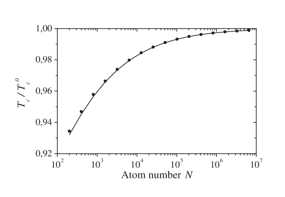
Figure 1: Critical temperature $T_{c}$ (normalized to $T_{c}^{0}$) for a finite number $N$ of atoms. The solid line is the analytical result given by (3), while the circles are given by numerically solving for $T$ the equation $N^{\prime}_{\rm max}(T)=N$. The agreement is excellent even for low values of $N$.

2.2 Interactions

The interatomic collisions in a tightly confined Bose gas have been studied in detail in [15]. We summarize in this section their main results. Similarly to the three-dimensional scattering problem, the scattering properties in two dimensions can be formulated by means of a single length $d^{*}$. This characteristic length depends on the detailed shape of the interatomic potential. For realistic momenta $q$ of particles in ultracold gases we always have the inequality $qd^{*}\ll 1$. The expression for the two-dimensional differential cross section for identical bosons reads: $d\sigma/d\theta(q)=|h(q)|^{2}/(4\pi q)$, where $q=m({\bf v}_{2}-{\bf v}_{1})/(2\hbar)$ is the relative wavevector of the colliding particles and the dimensionless function $h(q)$ depends logarithmically on $q$. The mean field potential in the non degenerate regime is $U({\bf r})=2gn({\bf r})$ with $n$ the density, $g=\hbar^{2}h(\bar{q})/m$ and $\bar{q}=(mk_{B}T)^{1/2}/\hbar$ the mean thermal wave vector.

The departure from the ideal gas behavior is measured through the ratio between the mean field energy and the level spacing. For weak interactions, namely $gn\ll\hbar\bar{\omega}$, interactions can be taken into account perturbatively and the physics of the ideal gas is valid. In the opposite limit $gn\gg\hbar\bar{\omega}$, interactions brings about major differences. One enters a regime of quasi-condensate [16]. From thermodynamics, one readily establishes the implicit equation for the density:

$$n({\bf r})=-\frac{1}{\lambda^{2}}\mbox{log}(1-\mbox{e}^{-\beta(U_{\rm trap}({\bf r})+2gn({\bf r})-\mu)}),$$ (4)

where $\lambda=h(2\pi mk_{B}T)^{-1/2}$ is the thermal de Broglie wavelength, $\beta=1/k_{B}T$ and $U_{\rm trap}$ is the trapping potential energy. Actually, in the non-perturbative interactions regime, the local density approximation is valid. Repulsive interactions tend to push the gas towards the external region, thereby reducing the density of the gas. One expects that this effect causes a natural decrease of the critical temperature. This is indeed the case and in contrast with its three dimensional counterpart, Eq. (4) is soluble at all temperatures [17]. To discriminate which state with or without condensate the system will prefer, the authors of Ref. [18] compare the free energy in both situations and predict that low-energy phonons destabilize the two-dimensional condensate. The nature of the phase in the degenerate regime remains somewhat an open question [19, 16, 18]. One may wonder if this state involves superfluidity at sufficently low temperature.

2.3 Expansion of the density

In on-going experiments on Bose-Einstein condensates of alkali atoms, the density profile is readily obtained by in situ images of the cloud. We give in this section the corrections to the density up to the second order due to the mean field contribution. However, this expansion is valid not too close to degeneracy. We expect that the repulsive mean field contributes to the decrease of the density. We capture this effect perturbatively by performing an expansion of the density profile with $\xi=2g\beta\lambda^{-2}$ as the small parameter. $\xi$ is the ratio between the mean field energy close to degeneracy and the temperature. By denoting $n^{(0)}_{0}$ the equilibrium density in absence of mean field, we work out the expansion:

$$n_{0}({\bf r})=n^{(0)}_{0}({\bf r})+\xi n^{(1)}_{0}({\bf r})+\xi^{2}n^{(2)}_{0}({\bf r})+...$$

$$n^{(0)}_{0}({\bf r})=-\lambda^{-2}\mbox{log}(1-\kappa)$$

$$n^{(1)}_{0}({\bf r})=-n^{(0)}_{0}\frac{\kappa}{1-\kappa}$$

$$n^{(2)}_{0}({\bf r})=-\frac{n^{(1)}_{0}}{1-\kappa}\bigg{(}\kappa-\frac{1}{2}\mbox{log}(1-\kappa)\bigg{)},$$ (5)

with $\kappa=\kappa({\bf r})=\exp(-\beta(U_{\rm trap}({\bf r})-\mu))$.

3 Dynamics

3.1 Quantum Boltzmann equation

The dynamics of the gas is described by a two-dimensional quantum Boltzmann equation:

$$\frac{\partial f}{\partial t}+{\bf v_{1}}\cdot\mbox{\boldmath$\nabla$}_{\bf r}f+\frac{{\bf F}}{m}\cdot\mbox{\boldmath$\nabla$}_{\bf v_{1}}f=I_{\rm coll}[f]$$ (6)

where $f$ is the phase space distribution function. The explicit form for the collision term is

$$I_{\rm coll}[f({\bf r},{\bf v_{1}})] \simeq \frac{m}{h}\frac{|h(\bar{q})|^{2}}{4\pi^{2}}\int d\theta\;d^{2}{v}_{2}\;\big{[}f({\bf r},{\bf v_{1^{\prime}}})f({\bf r},{\bf v_{2^{\prime}}})(1+f({\bf r},{\bf v_{1}}))(1+f({\bf r},{\bf v_{2}}))$$

$$-f({\bf r},{\bf v_{1}})f({\bf r},{\bf v_{2}})(1+f({\bf r},{\bf v_{1^{\prime}}}))(1+f({\bf r},{\bf v_{2^{\prime}}}))\big{]}$$

It accounts for elastic collisions between bosonic particles 1 and 2, with initial velocities ${\bf v_{1}}$ and ${\bf v_{2}}$, and final velocities ${\bf v_{1^{\prime}}}$ and ${\bf v_{2^{\prime}}}$, $\theta$ being the scattering angle in the center of mass frame. In the next sections, we first derive the expression for the collision rate with the interplay between statistics and mean field. Then, we investigate the role of collisions (mean field and relaxation) on the frequencies of the low-lying modes for a two-dimensional harmonic trap and we derive the equations for expansion after an abrupt switching off of the trap. The method used to solve those latter problems relies on a scaling ansatz. It is first introduced in the context of the collision-dominated hydrodynamic regime, and then adapted to the quantum Boltzmann equation [21].

3.2 Collision rate

The collision rate plays a crucial role for the relaxation dynamics, it permits to compare the mean free path to the size of the cloud and to characterize the collisional regime of the sample between collisionless and hydrodynamic. Well above the critical temperature, the mean field and the bosonic statistics can be neglected and the equilibrium distribution reads [20]:

$$f_{0}({\bf r},{\bf v})=N.\frac{\hbar\omega_{x}}{k_{B}T}.\frac{\hbar\omega_{y}}{k_{B}T}e^{-H_{0}({\bf r},{\bf v})/k_{B}T}$$ (7)

with

$$H_{0}({\bf r},{\bf v})=\frac{1}{2}m{\bf v}^{2}+\frac{1}{2}m\omega_{x}^{2}x^{2}+\frac{1}{2}m\omega_{y}^{2}y^{2}.$$ (8)

We readily obtain the expression for the collision rate $\gamma_{0}$ in this limit by integrating the first term of the collision integral of the classical Boltzmann equation for the equilibrium function $f_{0}$ and dividing by the number of particles:

$$\gamma_{0}=\frac{m^{3}}{h^{3}}\frac{|h(\bar{q})|^{2}}{2\pi N}\int d^{2}rd^{2}v_{1}\;d^{2}{v}_{2}\;f_{0}({\bf r},{\bf v}_{1})f_{0}({\bf r},{\bf v}_{2})=\frac{N\hbar\omega_{x}\omega_{y}}{4\pi k_{B}T}|h(\bar{q})|^{2}.$$ (9)

Closer to degeneracy but still above the critical temperature, one expects that the result is modified by two opposite effects. On the one hand, the mean field tends to decrease the density. On the other hand, the statistics tends to shrink the cloud. To evaluate the competition between those effects, we restrict ourselves in the following to the case of an isotropic harmonic confinement for sake of simplicity. We first expand the phase space distribution function: $f({\bf r},{\bf v})=f_{0}({\bf r},{\bf v})[1+f_{0}({\bf r},{\bf v})-2\beta gn_{0}({\bf r})]$. From the quantum Boltzmann equation, the collision rate can be expanded to the first order

$$\gamma = \frac{m^{3}}{h^{3}}\frac{|h(\bar{q})|^{2}}{4\pi^{2}N}\int d\theta\;d^{2}{v}_{2}\;d^{2}{v}_{1}\;d^{2}{r}\;f_{0}({\bf r},{\bf v_{1}})f_{0}({\bf r},{\bf v_{2}})\bigg{[}1+$$ (10)

$$f_{0}({\bf r},{\bf v_{1}})+f_{0}({\bf r},{\bf v_{2}})+f_{0}({\bf r},{\bf v_{1^{\prime}}})+f_{0}({\bf r},{\bf v_{1^{\prime}}})-4g\beta n_{0}({\bf r})\bigg{]}.$$

The signs in (10) clearly show the enhancement of the collision rate due to the statistics and its decrease due to the repulsive mean field. After a lengthy but straightforward calculation, we have worked out the explicit expression for the expansion of the collision rate with respect to statistics and mean field contribution:

$$\gamma=\gamma_{0}\bigg{[}1+\frac{2\pi^{2}}{9}\bigg{(}\frac{T_{c}^{0}}{T}\bigg{)}^{2}\bigg{(}1-\frac{gm}{\pi\hbar^{2}}\bigg{)}\bigg{]}.$$

Actually, the collision rate cannot be measured directly. However, all dissipative dynamics involve the collisions. We propose in the following to extract information on the collisional regime through the study of the collective oscillations or of the time-of-flight expansion, which can be both investigated experimentally.

3.3 Scaling ansatz for the hydrodynamic regime

In this section, we determine the frequencies of the collective oscillations of an harmonically trapped two-dimensional gas, and the equations for its time of flight when the confinement is switched off. For this purpose, we transpose the hydrodynamic approach developped in [22] for a three dimensional trapped Bose gas to a two-dimensional one. The scaling ansatz for the density reads: $n({\bf r},t)=n_{0}({\bf R}(t))/\Omega_{0}(t)$, where $n_{0}$ is the equilibrium density, ${\bf R}=A(t).{\bf r}$ with ${\bf r}$ the coordinate and $A(t)$ a diagonal matrix with time dependent scaling coefficient $A=\mbox{diag}(1/a_{x}(t),1/a_{y}(t))$. The parameter $a_{i}$ gives the dilation along the $i$th direction. One readily obtains $\Omega_{0}(t)=(\mbox{det}(A))^{-1}$ from the normalization $\int d^{2}rn({\bf r},t)=\int d^{2}rn_{0}({\bf r})$. Note that the scaling solution makes sense only if $A$ has non vanishing coefficients. The local hydrodynamic velocity field ${\bf v}^{\rm loc}$ is obtained from the ansatz for the density through the equation of continuity, which yields: ${\bf v}^{\rm loc}=-A^{-1}\dot{A}.{\bf r}$, where $\dot{A}=dA/dt$. The equations for the coefficients of the matrix $A$ are obtained from the Euler equation. For collective oscillations, we find the following set of nonlinear equations:

$$\ddot{a}_{x}+\omega_{x}^{2}a_{x}-\frac{\omega_{x}^{2}}{a_{x}^{2}a_{y}}=0\qquad\mbox{and}\qquad\ddot{a}_{y}+\omega_{y}^{2}a_{y}-\frac{\omega_{y}^{2}}{a_{y}^{2}a_{x}}=0.$$

For a small deviation from equilibrium, the linearization of the system leads to two hydrodynamic frequencies of oscillation:

$$\omega^{2}_{\pm}=\frac{\omega_{x}^{2}}{2}\bigg{[}3+3\beta^{2}\pm(9-14\beta^{2}+9\beta^{4})^{1/2}\bigg{]}$$

with $\beta=\omega_{y}/\omega_{x}$. For an isotropic trap ($\omega_{x}=\omega_{y}=\omega_{0}$), we find $\sqrt{2}\omega_{0}$ for the quadrupole mode and $2\omega_{0}$ for the monopole mode. For non isotropic trap, the two modes correspond to a superposition of the quadrupole and monopole modes. The equations for the time of flight in two dimensions are readily obtained in the same way:

$$\ddot{a}_{x}=\frac{\omega_{x}^{2}}{a_{x}^{2}a_{y}}\qquad\mbox{and}\qquad\ddot{a}_{y}=\frac{\omega_{y}^{2}}{a_{y}^{2}a_{x}}.$$

This set of equation shows that a high initial collision rate with respect to the trap frequencies (implicitly assumed for the validity of hydrodynamic equations) leads to an asymptotic anisotropic expansion [21].

3.4 Scaling ansatz for the Quantum Boltzmann Equation

In most cases the hydrodynamic formalism is not satisfactory for describing a Bose gas. Indeed, a time of flight expansion is accompanied by a dilution of the sample. As a result, the collision rate decreases. Hydrodynamic equations are mostly valid at the beginning of an expansion but certainly not after a long time [23]. We emphasize that the hydrodynamic regime is quite difficult to reach experimentally [24, 25] since a high collision rate means a high density for which the inelastic collision rate is magnified. However by exploiting Feshbach resonance, it has been possible recently to enter the hydrodynamic regime for fermionic gases in a three dimensional trap [26]. In order to take into account the evolution of the density one needs to solve at least approximately the Boltzmann equation. This equation permits us to describe the crossover between the collisionless and the hydrodynamic regime.

Following [21], we make the following ansatz for the distribution function: $f({\bf r},{\bf v},t)=f_{0}({\bf R},{\bf V})/\Omega(t)$ with $f_{0}$ the equilibrium distribution, ${\bf V}=B.({\bf v}-{\bf v}^{\rm loc})$, $B$ being a diagonal matrix $B=\mbox{diag}(1/b^{1/2}_{x}(t),1/b^{1/2}_{y}(t))$, and $\Omega(t)=\mbox{det}^{-1}(AB)$. The parameter $b_{i}$ gives the effective temperature in the $i$th direction and $f_{0}$ obeys the equilibrium Boltzmann equation:

$$\sum_{j}\bigg{(}V_{j}\frac{\partial f_{0}}{\partial R_{j}}-\omega_{j}^{2}R_{j}\frac{\partial f_{0}}{\partial V_{j}}-\frac{2g_{0}}{m}\frac{\partial n_{0}}{\partial R_{j}}\frac{\partial f_{0}}{\partial V_{j}}\bigg{)}=0,$$ (11)

where $n_{0}=(m^{2}/h^{2})\int d^{2}Vf_{0}$ is the equilibrium density and $g_{0}$ the strength of the interaction for the equilibrium temperature $T_{0}$. The scaling ansatz method does not provide an exact solution of the Boltzmann equation. However, it is in reasonable agreement with the numerical simulations based on molecular dynamics [21, 27] and with experiments [28]. By substituting the scaling ansatz for the distribution function in the Boltzmann equation and taking into account the properties of the equilibrium distribution Eq. (11) one obtains:

$$\frac{1}{\Omega}\sum_{i}\bigg{[}\bigg{(}\frac{b_{i}^{1/2}}{a_{i}}-\frac{g}{g_{0}}\frac{1}{a_{i}b_{i}^{1/2}}\frac{1}{\prod_{j}a_{j}}\bigg{)}V_{i}\frac{\partial f_{0}}{\partial R_{i}}-\bigg{(}\frac{\dot{b}_{i}}{2b_{i}}+\frac{\dot{a}_{i}}{a_{i}}\bigg{)}V_{i}\frac{\partial f_{0}}{\partial V_{i}}-$$

$$\bigg{(}\ddot{a}_{i}+\omega_{i}^{2}a_{i}-\frac{g}{g_{0}}\frac{\omega_{i}^{2}}{a_{i}}\frac{1}{\prod_{j}a_{j}}\bigg{)}\frac{R_{i}}{b^{1/2}_{i}}\frac{\partial f_{0}}{\partial V_{i}}\bigg{]}=I_{\rm coll}+\frac{\dot{\Omega}}{\Omega^{2}}f_{0}.$$ (12)

This way, we restrict further the solutions. Such an approach would fail for instance to take into account rotation in presence of the mean field. Eq. (12) gives constraints on the scaling coefficients $a_{i}$ and $b_{i}$. By denoting $\langle C\rangle_{0}=(m^{2}/h^{2})\int Cf_{0}({\bf R},{\bf V})d^{2}Rd^{2}V/N$, we readily derive the following set of equations by multiplying Eq. (12) respectively by $C=R_{i}V_{i}$ and $C=V_{i}^{2}$ and by performing the integration over the phase space:

$$\bigg{(}\frac{b_{i}}{a_{i}}-\frac{g}{g_{0}}\frac{1}{a_{i}}\frac{1}{\prod_{j}a_{j}}\bigg{)}\langle V_{i}^{2}\rangle_{0}+\bigg{(}\ddot{a}_{i}+\omega_{i}^{2}a_{i}-\frac{g}{g_{0}}\frac{\omega_{i}^{2}}{a_{i}}\frac{1}{\prod_{j}a_{j}}\bigg{)}\langle R_{i}^{2}\rangle_{0}=0$$

$$\frac{\dot{b}_{i}}{b_{i}}+2\frac{\dot{a}_{i}}{a_{i}}=\frac{m^{2}}{h^{2}}\frac{\Omega}{N\langle V_{i}^{2}\rangle_{0}}\int d^{2}Rd^{2}VV_{i}^{2}I_{\rm coll}.$$ (13)

In order to capture the physics of the collision integral, we treat this term within the relaxation approximation [21]. It allows us to recast the l.h.s of the last equation of (13) in the form:

$$\frac{m^{2}}{h^{2}}\frac{\Omega}{N\langle V_{i}^{2}\rangle_{0}}\int d^{2}Rd^{2}VV_{i}^{2}I_{\rm coll}=-\frac{1}{b_{i}}\bigg{(}\frac{b_{i}-b_{j}}{2\tau}\bigg{)}\qquad\mbox{with}\qquad i\neq j,$$

where $\tau$ is the relaxation time which corresponds to the average time between collisions. Using the properties of the equilibrium distribution, we finally obtain the following closed set of non linear equations for the scaling parameters:

$$\ddot{a}_{i}+\omega_{i}^{2}a_{i}-\omega_{i}^{2}\frac{b_{i}}{a_{i}}+\omega_{i}^{2}\xi\bigg{(}\frac{b_{i}}{a_{i}}-\frac{g}{g_{0}}\frac{1}{a_{i}}\frac{1}{\prod_{j}a_{j}}\bigg{)}=0$$

$$\dot{b}_{i}+2\frac{\dot{a}_{i}}{a_{i}}b_{i}=-\frac{1}{2\tau}(b_{i}-b_{j})\qquad\mbox{with}\qquad i\neq j,$$ (14)

with $\xi=g_{0}\langle n_{0}\rangle_{0}/(m\omega_{i}^{2}\langle R_{i}^{2}\rangle_{0})$. One recovers the collisionless regime by taking $\tau=\infty$. In this limit, we have a simple relation between $b_{i}$ and $a_{i}$: $b_{i}=a_{i}^{-2}$. In the opposite limit (hydrodynamic regime), local equilibrium is always ensured because of the high collision rate. As a consequence, the contribution of the collision integral vanishes because of local equilibrium and $b_{x}=b_{y}=1/(a_{x}a_{y})$. As the mean temperature is constant $g=g_{0}$, we recover in this limit the set of equations (3.3). In the next sections, we use this set of equations to derive the frequencies of the collective oscillations and we establish the equations for a time of flight expansion.

3.5 Collective oscillations

Low lying collective oscillations are reproduced by the time dependent dilatation parameters $a_{x}$ and $a_{y}$ of the trapped cloud around equilibrium. As a consequence, the temperature dependence of the interaction strength can be neglected $g=g_{0}$. To evaluate the relaxation time $\tau_{0}$, at least at equilibrium and in the high temperature limit, we perform a gaussian ansatz in the collision integral as explained in details in [27] for a three dimensional system. We find $\tau_{0}=2/\gamma_{0}$. Expanding Eqs. (14) around equilibrium ($a_{i}=b_{i}=1$) we get a linear closed set of equations which can be solved by searching for solutions of the type $e^{i\omega t}$. The associated determinant yields the dispersion law:

$$A[\omega]-\frac{i}{\tau_{0}}B[\omega]=0,$$ (15)

where $A[\omega]=\omega^{2}(\omega^{2}-\omega_{\rm cl+}^{2})(\omega^{2}-\omega_{\rm cl-}^{2})$, $B[\omega]=\omega(\omega^{2}-\omega_{\rm hd+}^{2})(\omega^{2}-\omega_{\rm hd-}^{2})$ and (cl) and (hd) refer to the collisionless and hydrodynamic regimes respectively. The values for $\omega^{2}_{\rm cl\pm}$ and $\omega^{2}_{\rm hd\pm}$ are given by

$$\omega^{2}_{\rm cl\pm} = \frac{\omega_{x}^{2}}{2}\bigg{[}(1+\beta^{2})(4-\xi)\pm\{(1+\beta^{2})^{2}(4-\xi)^{2}-32\beta^{2}(2-\xi)\}^{1/2}\bigg{]},$$

$$\omega^{2}_{\rm hd\pm} = \frac{\omega_{x}^{2}}{2}\bigg{[}3(1+\beta^{2})\pm\{9(1+\beta^{4})-14\beta^{2}\}^{1/2}\bigg{]},$$ (16)

with $\beta=\omega_{y}/\omega_{x}$.

The roots of $A$ that correspond to the collisionless regime in presence of mean field coincide with the one derived by [29]. The frequency of the monopole mode [29] for an isotropic trap ($\omega_{x}=\omega_{y}=\omega_{0}$) is found to be $2\omega_{0}$ whatever the collision regime. In two dimensions the collisions (mean field and relaxation) do not affect the frequency of this mode, this comes out from the fact that it is in the kernel of the integral of collision [27]. The symmetries of a two dimensional system for a contact interaction can explain this surprising result [30]. The hydrodynamic frequencies do not depend explicitly on the mean field, it is also a specific result of two dimensions low lying oscillations. As a consequence, the effect of the mean field upon collective oscillations is maximum in the crossover between collisionless and hydrodynamic regime.

3.6 Time of flight

In the following we investigate the evolution of the cloud in a time of flight. In this technique, the asymmetric trapping potential is switched off and the evolution of the spatial density is monitored. After a long time expansion, the aspect ratio gives information on the characteristics of the gas. Below the critical temperature, the anisotropic expansion is the favored signature of Bose-Einstein condensation. Actually, above the critical temperature and in the collisionless regime one expects an isotropic asymptotic expansion of the cloud reflecting the isotropy of the initial velocity distribution. However, anisotropic expansion also arises above the critical temperature, when the mean free path is small compared to the size of the cloud.

An analytic approach has been proposed in the full hydrodynamic regime [22] for a three dimensional Bose gas and has been adapted to a two dimensional gas in section 3.3. Alternatively, the expansion of an interacting Bose gas initially confined in a three dimensional trap above the critical temperature has been investigated by means of Monte Carlo simulations [31]. Two recent papers [21, 23] propose a way to provide an analytical interpolation between the two opposite collisionless and hydrodynamic regimes. The authors of Ref. [23] divide the expansion in two stages: the first one is considered as fully hydrodynamic and the second one as collisionless. The authors of Ref. [21] use a scaling ansatz to solve approximately the Boltzmann equation. We adapt in the following this latter method to a two dimensional gas.

The same procedure as the one used previously for the collective oscillations leads to the following set of equations:

$$\ddot{a}_{i}-\omega_{i}^{2}\frac{b_{i}}{a_{i}}+\omega_{i}^{2}\xi\bigg{(}\frac{b_{i}}{a_{i}}-\frac{g(\bar{b})}{g_{0}}\frac{1}{a_{i}}\frac{1}{\prod_{j}a_{j}}\bigg{)}=0$$

$$\dot{b}_{i}+2\frac{\dot{a}_{i}}{a_{i}}b_{i}=-\frac{1}{2\tau(a_{i})}(b_{i}-b_{j})\qquad\mbox{with}\qquad i\neq j,$$ (17)

where $\bar{b}=(b_{x}+b_{y})/2$. The confinement does not appear explicitly as in (14). The dependence with the parameters $a_{i}$ and $b_{i}$ of the collision term through the interaction strength $g$ and the time relaxation $\tau$ has to be taken into account. As recalled in section 2.2, $g$ depends logarithmically on the mean temperature $T=T_{0}\bar{b}$. Since the collision rate scales as the density, we deduce the scaling dependence of the relaxation time: $\tau=\tau_{0}\prod_{i}a_{i}$. During the expansion the scaling parameters $b_{i}$ decrease and as a consequence the gas cools down, revealing the isentropy of the expansion. By contrast with three-dimensional expansion, the mean field contribution is slightly magnified during the expansion through the dependence of $g$ upon the mean temperature. The persistence of the hydrodynamic expansion that may happen initially is more pronounced with respect to the three-dimensional case because of the more favorable dependence of the relaxation time on the scaling parameters.

4 Conclusion

In conclusion, our work shows that the coherent part of collisions included through a mean field term can manifest itself in various experimentally measurable ways already above the critical temperature: by modifying the frequencies of low-lying modes, or in competition with dissipative effects by producing an anisotropic expansion for an initially anisotropic trapping.

Appendix A Finite size effect on the critical temperature $T_{c}$

For $N$ bosons confined in a two-dimensional isotropic harmonic oscillator of angular frequency $\omega$, the critical temperature $T_{c}$ is the solution of the following equation

$$N=\sum_{n=1}^{\infty}\frac{n+1}{\exp[\hbar\omega n/(k_{B}T_{c})]-1}\,.$$ (18)

Since $T_{c}$ is close to $T_{c}^{0}=\hbar\omega\sqrt{6N}/(\pi k_{B})$, one has $\varepsilon\equiv\hbar\omega/(k_{B}T_{c})\sim N^{-1/2}\ll 1$.

We therefore expand Eq. (18) for $\varepsilon\ll 1$, retaining only the lowest order terms, up to $1/\varepsilon$. The sum can be replaced by an integral, provided we add a remainder $\mathcal{R}(\varepsilon)$ to keep an exact expression:

$$N=\int_{1}^{\infty}\frac{x+1}{\exp(\varepsilon x)-1}{\rm d}x+\mathcal{R}(\varepsilon)\,.$$ (19)

The expansion of the integral is straightforward

$$\int_{1}^{\infty}\frac{x+1}{\exp(\varepsilon x)-1}{\rm d}x=\frac{\pi^{2}}{6}\,\frac{1}{\varepsilon^{2}}-\frac{1}{\varepsilon}-\frac{\ln\varepsilon}{\varepsilon}+\mathcal{O}(1)\,$$ (20)

and the remainder can be evaluated with the Euler-McLaurin asymptotic formula [32]

$$\mathcal{R}(\varepsilon)=-\sum_{k=1}^{\infty}\frac{B_{k}}{k!}f^{(k-1)}(1)\,\,\,\,\,{\rm with}\,\,\,\,\,f(x)=\frac{x+1}{\exp(\varepsilon x)-1}$$ (21)

where $B_{k}$ is the $k$th Bernoulli number. One then expands the derivatives of $f$ up to order $1/\varepsilon$, and one finds:

$$\mathcal{R}(\varepsilon)=\frac{S}{\varepsilon}+\mathcal{O}(1),$$ (22)

where the coefficient $S$ is given by the following series:

$$S=1+1/12-1/120+1/252+\cdots$$ (23)

which turns out to be a diverging series. Nevertheless, retaining only a finite number of terms of this series actually gives a very good approximation [33] of the value of $S\simeq 1.079\pm 0.003$. Therefore,

$$N=\frac{\pi^{2}}{6}\,\frac{1}{\varepsilon^{2}}+\frac{0.079}{\varepsilon}-\frac{\ln\varepsilon}{\varepsilon}+\mathcal{O}(1)\,.$$ (24)

Substituting $\varepsilon$ by $\sqrt{\pi^{2}/6N}(1-\delta T_{c}/T_{c}^{0})$ in the previous equation, and expanding up to first order in $\delta T_{c}/T_{c}^{0}$ finally yields the shift of critical temperature:

$$\frac{\delta T_{c}}{T_{c}^{0}}\simeq-\frac{0.195\ln N-0.066}{\sqrt{N}}\,.$$ (25)

References

- [1] A.I. Safonov, S.A. Vasilyev, I.S. Yasnikov, I.I. Lukashevich, and S. Jaakkola, Phys. Rev. Lett. 81, 4545 (1998).
- [2] J.T.M. Walraven, in Fundamental Systems in Quantum Optics, Proceedings of the Les Houches Summer School, Session LIII, edited by J. Dalibard, J.M. Raimond, and J. Zinn-Justin (Elsevier Science Publishers, Amsterdam, 1992).
- [3] V.L. Berezinski, Sov. Phys. JETP 32, 493 (1971); V.L. Berezinski, Sov. Phys. JETP 34, 610 (1972).
- [4] J.M. Kosterlitz and D.J. Thouless, J. Phys. C 6, 1181 (1973); J.M. Kosterlitz, J. Phys. C 7, 1046 (1974).
- [5] N. Prokof ev, O. Ruebenacker, and B. Svistunov, Phys. Rev. Lett. 87, 270402 (2001).
- [6] V. Vuletić, C. Chin, A.J. Kerman, and S. Chu, Phys. Rev. Lett 81, 5768 (1998); I. Bouchoule, H. Perrin, A. Kuhn, M. Morinaga, and C. Salomon, Phys. Rev. A 59, 8(R) (1999); S. Burger, F. S. Cataliotti, C. Fort, P. Maddaloni, F. Minardi and M. Inguscio, Europhys. Lett. 57, 1 (2002); I. Bouchoule, M. Morinaga, C. Salomon, and D. Petrov Phys. Rev. A 65, 033402 (2002).
- [7] A. Görlitz, J.M. Vogels, A.E. Leanhardt, C. Raman, T.L. Gustavson, J.R. Abo-Shaeer, A.P. Chikkatur, S. Gupta, S. Inouye, T. Rosenband, and W. Ketterle, Phys. Rev. Lett. 87, 130402 (2001).
- [8] M. Hammes, D. Rychtarik, B. Engeser, H.-C. Nägerl, and R. Grimm, Phys. Rev. Lett. 90, 173001 (2003).
- [9] D. Rychtarik, B. Engeser, H.-C. N gerl and R. Grimm, cond-mat/0309536.
- [10] O. Zobay and B.M. Garraway, Phys. Rev. Lett. 86, 1195 (2001); O. Zobay and B.M. Garraway cond-mat:0306198.
- [11] to appear in the proceedings of the school Quantum gases in low dimensions at Les Houches 15-25 april 2003, Journal de Physique IV (EDP Sciences) 2003.
- [12] V. Bagnato and D. Kleppner, Phys. Rev. A 44, 7439 (1991).
- [13] W. Ketterle and N.J. van Druten, Phys. Rev. A 54, 656 (1996);
- [14] W.J. Mullin, J. Low. Temp. Phys. 106, 615 (1997).
- [15] D.S. Petrov and G.V. Shlyapnikov, Phys. Rev. A 64, 012706 (2001).
- [16] D.S. Petrov, M. Holzmann, and G.V. Shlyapnikov, Phys. Rev. Lett. 84, 2551 (2000).
- [17] R.K. Bhaduri, S.M. Reimann, S. Viefers, A. Ghose Choudhury, J. Phys. B 33, 3895 (2000).
- [18] J.P. Fernández and W.J. Mullin, J. Low. Temp. Phys. 128, 233 (2002).
- [19] W.J. Mullin, J. Low. Temp. Phys. 110, 167 (1998); W.J. Mullin, M. Holzmann and F. Laloë, ibid 121, 263 (2000); W.J. Mullin, M. Holzmann and F. Laloë, ibid 121, 269 (2000).
- [20] We choose the following normalization .
- [21] P. Pedri, D. Guéry-Odelin and S. Stringari, Phys. Rev. A. 68, 043608 (2003).
- [22] Yu. Kagan, E.L. Surkov and G.V. Shlyapnikov, Phys. Rev. A 55, R18 (1997).
- [23] I. Shvarchuck, Ch. Buggle, D.S. Petrov, M. Kemmann, W. von Klitzing, G.V. Shlyapnikov, and J.T.M. Walraven, arXiv:cond-mat/0308493.
- [24] D. M. Stamper-Kurn, H.-J. Miesner, S. Inouye, M. R. Andrews, W. Ketterle, Phys. Rev. Lett. 81, 500 (1998)
- [25] M. Leduc, J. Léonard, F. Pereira dos Santos, E. Jahier, S. Schwartz and C. Cohen-Tannoudji, Acta Physica Polonica B 33, 2213 (2002).
- [26] T. Bourdel, J. Cubizolles, L. Khaykovich, K.M.F. Magalhães, S.J.J.M.F. Kokkelmans, G.V. Shlyapnikov, and C. Salomon, Phys. Rev. Lett. 91 020402 (2003).
- [27] D. Guéry-Odelin, F. Zambelli, J. Dalibard and S. Stringari, Phys. Rev. A 60, 4851 (1999).
- [28] F. Gerbier, J.H. Thywissen, S. Richard, M. Hugbart, P. Bouyer and A. Aspect, arXiv:cond-mat/0307188.
- [29] D. Guéry-Odelin, Phys. Rev. A 66, 033613 (2002).
- [30] L.P. Pitaevskii and A. Rosch, Phys. Rev. A 55, R853 (1997).
- [31] H. Wu and E. Arimondo, Europhys. Lett. 43, 141 (1998).
- [32] W.H. Press, S.A. Teukolsky, W.T. Vetterling, B.P. Flannery, Numerical Recipes in C, (2nd Edition, Cambridge University Press, 1992).
- [33] As explained in [32], 4.2, the error is smaller than the first neglected term of the Euler-McLaurin series.