Level Statistics of XXZ Spin Chains with Discrete Symmetries: Analysis through Finite-size Effects

Abstract

Level statistics is discussed for XXZ spin chains with discrete symmetries for some values of the next-nearest-neighbor (NNN) coupling parameter. We show how the level statistics of the finite-size systems depends on the NNN coupling and the XXZ anisotropy, which should reflect competition among quantum chaos, integrability and finite-size effects. Here discrete symmetries play a central role in our analysis. Evaluating the level-spacing distribution, the spectral rigidity and the number variance, we confirm the correspondence between non-integrability and Wigner behavior in the spectrum. We also show that non-Wigner behavior appears due to mixed symmetries and finite-size effects in some nonintegrable cases.

1 Introduction

Statistical properties of energy levels have been studied for various physical systems in terms of the random matrix theory (RMT). For quantum systems, the RMT analysis has been applied to characterize quantum chaos and to investigating the integrability of a system. For quantum spin systems, we adopt a definition of integrability by the Bethe ansatz: an integrable model is exactly solvable by the Bethe ansatz. Since a pioneering work [1], the following conjecture has been widely accepted: If a given Hamiltonian is integrable by the Bethe ansatz, the level-spacing distribution should be described by the Poisson distribution:

$$P_{\rm Poi}(s)=\exp(-s).$$ (1)

If it is nonintegrable, the level-spacing distribution should be given by the Wigner distribution, i.e. the Wigner surmise for the Gaussian orthogonal ensemble (GOE):

$$P_{\rm Wig}(s)=\frac{\pi s}{2}\exp\left(-\frac{\pi s^{2}}{4}\right).$$ (2)

In principle, the conjecture is valid only for thermodynamically large systems. Furthermore, there is no theoretical support for the conjecture for quantum systems. However, we shall show that it is practically effective for finite-size quantum systems. In fact, the above conjecture has been numerically confirmed for many quantum spin systems such as correlated spin systems [1, 2, 3, 4, 5, 6, 7] and disordered spin systems [8, 9, 10, 11, 12]. In the Anderson model of disordered systems, $P_{\rm Poi}(s)$ and $P_{\rm Wig}(s)$ characterize the localized and the metallic phases, respectively. [13]

It is important to study statistical properties of energy levels for XXZ spin chains, which are related to various important quantum spin chains as well as classical lattice models in two dimensions. Let us consider a spin-$\frac{1}{2}$ XXZ spin chain on $L$ sites with next-nearest-neighbor (NNN) interaction

$$\mathcal{H}=J_{1}\sum^{L}_{j=1}(S^{x}_{j}S^{x}_{j+1}+S^{y}_{j}S^{y}_{j+1}+\Delta_{1}S^{z}_{j}S^{z}_{j+1})+J_{2}\sum^{L}_{j=1}(S^{x}_{j}S^{x}_{j+2}+S^{y}_{j}S^{y}_{j+2}+\Delta_{2}S^{z}_{j}S^{z}_{j+2}),$$ (3)

where $S^{\alpha}=(1/2)\sigma^{\alpha}$ and $(\sigma^{x},\sigma^{y},\sigma^{z})$ are the Pauli matrices; the periodic boundary conditions are imposed. The Hamiltonian (3) is nonintegrable when the NNN coupling $J_{2}$ is nonzero, while it is integrable when $J_{2}$ vanishes. Here we also note that it coincides with the NNN coupled Heisenberg chain when $\Delta_{1}=\Delta_{2}=1$. When $J_{2}$ vanishes the system becomes the integrable XXZ spin chain, which is one of the most important integrable quantum spin chains. Here, quantum integrability should lead to Poisson behavior as the characteristic behavior of level statistics. When $J_{2}$ is nonzero, the characteristic behavior of level statistics should be given by Wigner behavior. Here we note that the NNN interaction gives rise to frustration among nearest neighboring and next-nearest neighboring spins, which should lead to some chaotic behavior in the spectrum. [14] In a previous research, however, unexpected behavior of level-spacing distributions has been found for NNN coupled XXZ spin chains. [6] Robust non-Wigner behavior has been seen, although the NNN coupled chains are nonintegrable. The non-Wigner behavior of level-spacing distributions appears particularly when total $S^{z}$ ($S^{z}_{\rm tot}$)$=0$, and is roughly given by the average of $P_{\rm Poi}(s)$ and $P_{\rm Wig}(s)$. Similar non-Wigner behavior has been observed for a circular billiard when the angular momentum $L_{z}=0$, and for an interacting two-electron system with the Coulomb interaction in a quantum billiard when $L_{z}=0$. [15] Here we should note that Wigner behavior has been discussed in ref. rabson for some XXZ spin chains in sectors of $S^{z}_{\rm tot}\neq 0$.

In this paper we show that finite-size effects and discrete symmetries are important for analyzing the level statistics of XXZ spin chains. We show explicitly how the characteristic property of level statistics of the XXZ spin chains depends on the NNN coupling, the XXZ anisotropy and the system size. It is nontrivial to confirm the conjecture for finite XXZ spin chains which have the integrable line and some higher symmetrical points in the parameter space. Numerically we discuss that the characteristic behavior of level statistics is determined through competition among quantum chaos, integrability and finite-size effects. We confirm the correspondence between non-integrability and Wigner behavior in the spectrum. We also discuss why the unexpected non-Wigner behavior has appeared for $S^{z}_{\rm tot}=0$ in ref. NNN. We explicitly consider two aspects such as mixed symmetry and some finite-size effects. Furthermore, in various cases we show under what conditions non-Wigner behavior appears due to the two aspects. It seems to be rare that such various cases of non-Wigner behavior have been completely understood.

There is another motivation for the present research: another unexpected behavior of level-spacing distribution has been found for the integrable XXZ chain in ref. NNN. The level-spacing distribution $P(s)$ has shown a novel peak at $s=0$ for the anisotropy parameter $\Delta_{1}=0.5$. The appearance of the peak is consistent with the $sl_{2}$ loop algebra symmetry which appears only for special values of $\Delta_{1}$. Here we do not consider $\Delta_{2}$ since $J_{2}=0$. Let us introduce a parameter $q$ through the relation $\Delta_{1}=(q+1/q)/2$. When $q$ is a root of unity, the integrable XXZ Hamiltonian commutes with the $sl_{2}$ loop algebra. [16] Here the loop algebra is an infinite-dimensional Lie algebra, and the dimensions of some degenerate eigenspaces increase exponentially with respect to the system size. [17, 18] Thus the degenerate multiplicity of the non-Abelian symmetry can be extremely large. Furthermore, the $sl_{2}$ loop algebra is closely related to Onsager’s algebra [19] through which the Ising model was originally solved for the first time. The XXZ spin chains are thus closely related to the most important families of integrable systems through the integrable point, while they are also extended into nonintegrable systems quite naturally. We may therefore expect that the RMT analysis of the XXZ spin chains is important in discussing level statistics for other quantum systems that have some connection to an integrable system.

The organization of this paper is the following. In $\S$ 2, we recall some aspects of numerical procedure for level statistics. In particular, we explain desymmetrization of the XXZ Hamiltonian. We also remark that in the paper we consider only the XY-like region where $|\Delta|\leq 1$ for $\Delta=\Delta_{1}$ and $\Delta=\Delta_{2}$. In $\S$ 3, we show how competition among quantum chaos, quantum integrability and finite-size effects appears in the level statistics of the NNN coupled XXZ spin chains. We evaluate level-spacing distributions, spectral rigidities, and number variances, and confirm the RMT correspondence between non-integrability and Wigner behavior in the spectrum. We solve the non-Wigner behavior reported in ref. NNN and show how the behavior of level statistics changes due to mixed symmetry and finite-size effects. We also show that the characteristic behavior of level statistics does not depend on the energy range. This makes remarkable contrast to the level statistics of spinless fermions evaluated in the low energy spectrum at $1/3$ filling, [20] as well as to that of the Anderson model evaluated at edge regions of spectrum. In $\S$ 4 we discuss level statistics for a special case of the integrable XXZ spin chain where it has the $sl_{2}$ loop algebra symmetry. We observe that there remains many spectral degeneracies in the sector of $S^{z}_{\rm tot}=0$ even after desymmetrization with respect to spin reversal symmetry. Finally, we give conclusions in $\S$ 5.

2 Numerical Procedure

Let us discuss desymmetrization of the Hamiltonians of the XXZ spin chains. When performing calculation on level statistics, one has to separate the Hamiltonian matrices into some sectors; in each sector, the eigenstates have the same quantum numbers. The NNN coupled XXZ chains are invariant under spin rotation around the $z$-axis, translation, reflection, and spin reversal. Therefore we consider quantum numbers for the total $S^{z}$ ($S^{z}_{\rm tot}$), the total momentum $K_{\rm tot}$, the parity, and the spin reversal. However the total momentum $K_{\rm tot}$ is invariant under reflection only when $K_{\rm tot}=0$ or $\pi$. Thus the desymmetrization according to parity is performed only when $K_{\rm tot}=0$ or $\pi$. Similarly, $S^{z}_{\rm tot}$ is invariant under spin reversal only when $S^{z}_{\rm tot}=0$. Thus the desymmetrization according to spin reversal is performed only when $S^{z}_{\rm tot}=0$.

It is convenient to use a momentum-based form for the Hamiltonian when we calculate eigenvalues of the NNN coupled chains. To obtain the form, we perform the Jordan-Wigner and the Fourier transformations on the original spin Hamiltonian. Some details are explained in Appendix A. To calculate the eigenvalues, we use standard numerical methods, which are contained in the LAPACK library.

To find universal statistical properties of the Hamiltonians, one has to deal with unfolded eigenvalues instead of raw eigenvalues. The unfolding method is detailed in refs. NNN and random.

To analyze spectral properties, in this paper, we calculate three quantities: level-spacing distribution $P(s)$, spectral rigidity $\Delta_{3}(l)$, and number variance $\Sigma^{2}(l)$. The level-spacing distribution is the probability function $P(s)$ of nearest-neighbor level-spacing $s=x_{i+1}-x_{i}$, where $x_{i}$’s are unfolded eigenvalues. The level-spacing distribution is calculated over the whole spectrum of unfolded eigenvalues unless we specify the range. The spectral rigidity is given by

$$\Delta_{3}(l)=\left\langle\frac{1}{l}\min_{a,b}\int^{\varepsilon_{0}+l/2}_{\varepsilon_{0}-l/2}[N_{u}(\varepsilon)-a\varepsilon-b]^{2}d\varepsilon\right\rangle_{\varepsilon_{0}},$$ (4)

where $N_{u}(\varepsilon)=\Sigma_{i}\theta(\varepsilon-\varepsilon_{i})$ is the integrated density of unfolded eigenvalues and $\langle\rangle_{\varepsilon_{0}}$ denotes an average over $\varepsilon_{0}$. The average is done on the whole spectrum except about 15 levels on each side of the spectrum. The expression of $\Delta_{3}(l)$ gives the least square deviation of $N_{u}(\varepsilon)$ from the best fit straight line in an interval $l$. The number variance is given by

$$\Sigma^{2}(l)=\left\langle\left[N_{u}\left(\varepsilon_{0}+\frac{l}{2}\right)-N_{u}\left(\varepsilon_{0}-\frac{l}{2}\right)-l\right]^{2}\right\rangle_{\varepsilon_{0}},$$ (5)

where $\langle\rangle_{\varepsilon_{0}}$ denotes an average over $\varepsilon_{0}$. [21] The average is done on the whole spectrum except about 10 levels on each side of the spectrum.

We calculate the spectrum for the 18-site chains with NNN couplings. The matrix size is given by the following: $1387\times 1387$ for $S^{z}_{\rm tot}=0$ and $K_{\rm tot}=0$ (Here desymmetrization is performed except for spin reversal); $1364\times 1364$ for $S^{z}_{\rm tot}=0$ and $K_{\rm tot}=2\pi/L$, where $L$ is the number of sites (Here desymmetrization is performed also for spin reversal); $1282\times 1282$ for $S^{z}_{\rm tot}=1$ and $K_{\rm tot}=0$.

Numerical calculations are performed for the $XY$-like region, $|\Delta|<1$, where $\Delta$ is the anisotropic parameter $\Delta_{1}$ or $\Delta_{2}$. It may be interesting to study for the Ising-like region, $|\Delta|>1$, because there exist Ising-like magnets. For example, CsCoBr₃ and CsCoCl₃ are quasi-1D Ising-like antiferromagnets with $\Delta\sim 10$. [22] For $\Delta\gg 1$, however, level statistics is not reliable because energy spectra have some large gaps relative to $\Delta$ and the above unfolding method is invalid.

3 Next-Nearest-Neighbor Coupled XXZ Spin Chains

We now discuss numerically in the section that for the XXZ spin chains the characteristic behavior of level statistics is determined through competition among quantum chaos, quantum integrability and finite-size effects.

3.1 Spin reversal symmetry and Wigner behavior for $S_{tot}^{z}=0$

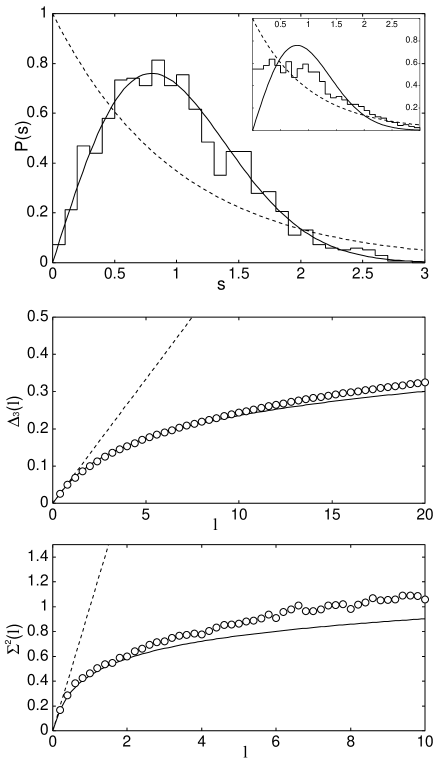
Figure 1: Level-spacing distribution $P(s)$, spectral rigidity $\Delta_{3}(l)$, and number variance $\Sigma^{2}(l)$ of the NNN coupled chain for $L=18$, $J_{2}/J_{1}=0.5$, $\Delta_{1}=\Delta_{2}=0.5$, $S^{z}_{\rm tot}=0$, $K_{\rm tot}=2\pi/L$ under complete desymmetrization. Broken lines correspond to Poisson behavior, and solid curves Wigner behavior. The inset shows $P(s)$ of the same system under incomplete desymmetrization. Namely, the desymmetrization with respect to spin reversal symmetry is not performed for the inset.

For a sector of $S^{z}_{\rm tot}=0$ we numerically discuss the characteristic behavior of level statistics on the XXZ spin chains. Here we note that spin reversal symmetry has not been considered explicitly in previous studies of level statistics for various quantum spin chains. In some sense, desymmetrizing the Hamiltonian with respect to spin reversal symmetry has been avoided due to some technical difficulty. Level statistics has been discussed only for sectors of $S^{z}_{\rm tot}\neq 0$, where there is no need of the desymmetrization with respect to spin reversal symmetry.

Let us show explicitly such a case that Wigner behavior appears for $S^{z}_{\rm tot}=0$ if we consider spin reversal symmetry. In Fig. 1 we have obtained the numerical results for level statistics such as the level-spacing distribution $P(s)$, the spectral rigidity $\Delta_{3}(l)$ and the number variance $\Sigma^{2}(l)$, for the sector of $K_{\rm tot}=2\pi/L$ and $S_{\rm tot}^{z}=0$. Here we note that in the sector parity invariance does not exist and we focus on spin reversal symmetry. The numerical results of level statistics shown in Fig. 1 clearly suggest Wigner behavior. The curve of the Wigner distribution fits well to the data of the level-spacing distribution $P(s)$ in the main panel. The plots of the spectral rigidity $\Delta_{3}(l)$ are consistent with the curve of Wigner behavior especially for small $l$ as shown in Fig. 1. It is also the case with the number variance $\Sigma^{2}(l)$. We see small deviations of $\Delta_{3}(l)$ and $\Sigma^{2}(l)$ for large $l$ because of some finite-size effects. We have thus confirmed that Wigner behavior appears also in the sector of $S_{\rm tot}^{z}=0$ for the XXZ spin chains with the NNN interaction.

In the inset of Fig. 1, we have shown the level-spacing distribution for which we do not perform the desymmetrization with respect to spin reversal. It shows non-Wigner behavior, which is similar to that of some other cases of mixed symmetry as we shall show in Fig. 4.

The spin reversal operation on the spin variable of the $j$th site is defined by

$$S^{\pm}_{j}\to S^{\mp}_{j},\quad S^{z}_{j}\to-S^{z}_{j}.$$ (6)

Here, $S^{\pm}_{j}=(S^{x}_{j}\pm{\rm i}S^{y}_{j})/2$. Let $M$ denote the number of down-spins in a given sector. The value of the total spin operator $S_{\rm tot}^{z}$ is given by $S_{\rm tot}^{z}=L/2-M$. Some details of spin reversal operation are given in Appendices B and C.

3.2 Finite-size effects on the level-spacing distribution

Let us explicitly discuss finite-size effects appearing in level statistics. They are important in the Poisson-like or non-Wigner behavior observed in level statistics for the completely desymmetrized XXZ Hamiltonians. There are two regions in which finite-size effects are prominent: A region where $J_{2}$ is close to zero and another region where $\Delta_{1}$ and $\Delta_{2}$ are close to 1. In the former region quantum integrability appears through finite-size effects, and the characteristic behavior of level statistics becomes close to Poisson-like behavior. In the latter region, Poisson-like behavior appears due to the symmetry enhancement at the point of $\Delta_{1}=\Delta_{2}=1$, where the $U(1)$ symmetry of the XXZ spin chain expands into the spin $SU(2)$ symmetry.

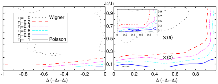
Figure 2: The diagram of contour lines of $\eta$ for the NNN coupled chain with $L=18$ (in the inset, $L=16$), in the sector of $S^{z}_{\rm tot}=1$ and $K_{\rm tot}=0$. Roughly speaking, the area above the thick long-dashed line, Wigner behavior; the area below the thick solid line, Poisson behavior. The points (a) and (b) correspond to Figs. 3(a) and 3(b), respectively.

Let us now discuss how the degree of non-Wigner behavior depends on the anisotropy parameters, $\Delta_{1}$ and $\Delta_{2}$, and the NNN coupling, $J_{2}$. For simplicity we set $\Delta_{1}=\Delta_{2}$ and denote it by $\Delta$, and we also consider the ratio of $J_{2}/J_{1}$. We express the degree of non-Wigner behavior by the following parameter:

$$\eta=\frac{\int^{s_{0}}_{0}[P(s)-P_{\rm Wig}(s)]ds}{\int^{s_{0}}_{0}[P_{\rm Poi}(s)-P_{\rm Wig}(s)]ds},$$ (7)

where $s_{0}=0.4729\cdots$ is the intersection point of $P_{\rm Poi}(s)$ and $P_{\rm Wig}(s)$. [9, 12] We have $\eta=0$ when $P(s)$ coincides with $P_{\rm Wig}(s)$, and $\eta=1$ when $P(s)$ coincides with $P_{\rm Poi}(s)$. The diagram of contour lines of $\eta$ is shown in Fig. 2. We have calculated them for the area $-0.98\leq\Delta\leq-0.02$, $0.02\leq\Delta\leq 0.98$, and $0.02\leq J_{2}/J_{1}\leq 1$, where $\Delta=\Delta_{1}=\Delta_{2}$.

The contour lines of $\eta$ show that a behavior close to Wigner one appears in a large region, while the Poisson-like behavior appears in a narrow region along the line of $J_{2}/J_{1}=0$ and that of $\Delta_{1}=\Delta_{2}=1$. The Poisson-like behavior is dominated by finite-size effects and hence should vanish when $L\to\infty$. This expectation is consistent with the suggestion in ref. rabson that an infinitesimal integrability-breaking term (the NNN term of eq. (3) in this paper) would lead to Wigner behavior. In fact, it is seen in the inset of Fig. 2 that the region of Wigner behavior shrinks for $L=16$. Here we remark that the phase diagrams of the ground state [23, 24] are totally different from the diagram of contour lines of $\eta$. It is due to the fact that level statistics reflects highly excited states rather than the ground state.

When $\Delta_{1}=\Delta_{2}=0.98$, Poisson-like behavior appears in level statistics due to some finite-size effects. It will be explicitly shown in Figs. 4 and 5. When $\Delta_{1}=\Delta_{2}=1$, eq. (3) coincides with the Heisenberg chain, which has the spin $SU(2)$ symmetry. Some degenerate energy levels at $\Delta_{1}=\Delta_{2}=1$ can become nondegenerate when $\Delta_{1}$ and $\Delta_{2}$ are not equal to 1. The difference among the nondegenerate energy levels should be smaller than the typical level spacing when $\Delta_{1}$ and $\Delta_{2}$ are close to 1. The typical level spacing, which is of the order of $1/L$, should become large when the system size $L$ is small. Thus, the Poisson-like behavior should practically appear in level statistics. We note that for the Heisenberg chain Wigner behavior appears in the level-spacing distribution when we desymmetrize the Hamiltonian with respect to the spin $SU(2)$ symmetry. [2, 3]

3.3 Homogeneity of the characteristic behavior of level statistics throughout the spectrum

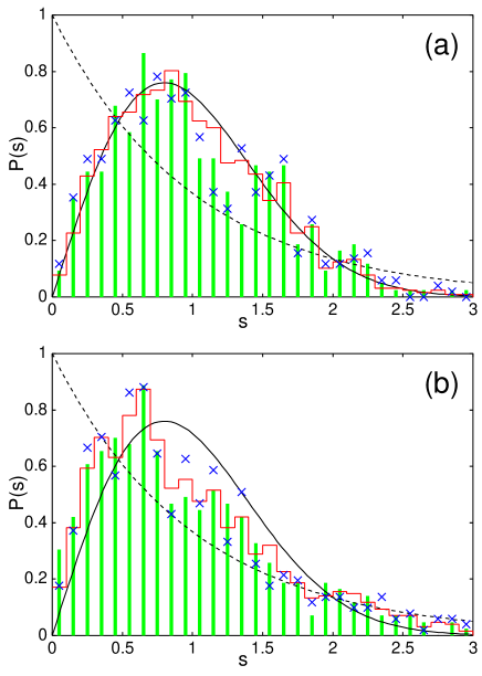
Figure 3: Level-spacing distribution of the NNN coupled chain for $L=18$, $\Delta_{1}=\Delta_{2}=0.5$, $S^{z}_{\rm tot}=1$, and (a) $J_{2}/J_{1}=0.5$; (b) $J_{2}/J_{1}=0.2$. Red histograms are for all levels; green bars, $1/3$ of all levels around the center; blue crosses, 10% of all levels from each of the two edges. Solid and broken lines show the Wigner and Poisson distributions, respectively.

Let us discuss that for the XXZ spin chains the characteristic behavior of level statistics does not depend on the energy range of the spectrum. In Fig. 3, we show level-spacing distributions evaluated at points (a) and (b) shown in the diagram of Fig. 2. They are evaluated for three different energy ranges. The distributions shown in Fig. 3(a) give Wigner behavior, while the distributions of Fig. 3(b) are close to Poisson behavior.

Let us explain the three different energy ranges shown in Fig. 3. Histograms show the level-spacing distributions evaluated for all levels, while bars show those evaluated only for the $1/3$ of all levels around the center, and crosses for the 10% of all levels located from each of the two spectral edges.

Quite interestingly, the distributions evaluated for the different energy ranges are quite similar to each other. It should be typical of frustrated quantum systems. In frustrated quantum systems, quantum chaotic behavior appears already in the low energy region near the ground state. [14] For non-frustrated cases, however, level statistics shows Poisson-like behavior in a low region. In ref. Zotos, for example, level statistics is Poisson-like for the low energy spectrum of one-dimensional spinless fermions with the nearest hopping, the nearest- and next-nearest-neighbor interactions in a $1/3$-filling case. The model is related to our model by a transformation, while, the $1/3$-filling case is not a frustrated case. Furthermore, there is another example of Poisson behavior. The level statistics of the Anderson model shows Poisson behavior even in the metallic phase, if we evaluate it in the edge regions of energy spectrum.

3.4 Two solutions to unexpected non-Wigner behavior: mixed symmetry and finite-size effects

Unexpected non-Wigner behavior has been reported in ref. NNN for level-spacing distributions of the NNN coupled XXZ chains. Let us discuss the reason why it was observed, considering both mixed symmetry and finite-size effects. Here we explain mixed symmetry in the following: Suppose that the Hamiltonian of a system is invariant under symmetry operations $T_{j}$ for $j=1,2,\ldots,m$, which are commuting each other. The eigenstates of the Hamiltonian are specified by the set of the eigenvalues of all $T_{j}$. If we desymmetrize the spectrum with respect to a partial set of symmetry operations, we say that the derived spectrum has mixed symmetry. For instance, if we only consider symmetry operations $T_{j}$ for $j=1,2,\ldots,m-1$, then the contributions of such eigenstates with different eigenvalues of $T_{m}$ can be mixed in the derived spectrum.

There are two types of non-Wigner profiles reported in ref. NNN for the nonintegrable systems: one is given by almost the numerical average of the Poisson and the Wigner distributions, and another one is rather close to the Poisson distribution. The profiles of the first type appear in various cases, [6] such as the case of $\Delta_{2}=0.5$. The profiles of the second type appear in particular for the case of $\Delta_{1}\simeq\Delta_{2}\simeq 1$. We may call the latter Poisson-like behavior rather than simple non-Wigner behavior. Both types of non-Wigner distributions have been observed in the subspace of $S^{z}_{\rm tot}=0$, which is the largest sector of the Hamiltonian matrix of eq. (3). Here we note that the observations in ref. NNN are obtained particularly for $S^{z}_{\rm tot}=0$, while in ref. rabson the Wigner behavior is observed for $S^{z}_{\rm tot}\neq 0$ in the level-spacing distributions of similar XXZ chains.

Figure 4: Level-spacing distribution $P(s)$ of the NNN coupled chain for $L=18$, $J_{2}/J_{1}=1$, $K_{\rm tot}=0$. Broken lines, the Poisson distribution; solid curves, the Wigner distribution.

We give level-spacing distributions in Fig. 4 for the four cases: $S^{z}_{\rm tot}=0$ or $1$ and $\Delta_{1}=\Delta_{2}=0.5$ or $0.98$. The numerical results suggest that the value of $S^{z}_{\rm tot}$ should be important as well as the anisotropy parameters, $\Delta_{1}$ and $\Delta_{2}$, in the observed non-Wigner behavior of the level-spacing distributions. When $\Delta_{1}=\Delta_{2}=0.5$, Wigner behavior appears for $S^{z}_{\rm tot}=1$, while the non-Wigner behavior was observed for $S^{z}_{\rm tot}=0$. We have also checked that Wigner behavior appears for $S^{z}_{\rm tot}=2$. Furthermore, we have confirmed that such $S^{z}_{\rm tot}$-dependence of the level-spacing distribution is valid for some values of $K_{\rm tot}$. Here we have desymmetrized the Hamiltonian according to $S^{z}_{\rm tot}$, $K_{\rm tot}$, and the parity when it exists, but not to the spin reversal. Here we note that the parity invariance exists only for sectors with $K_{\rm tot}=0$ or $\pi$ when $L$ is even.

The non-Wigner behavior observed for the case $S^{z}_{\rm tot}=0$ and $\Delta_{1}=\Delta_{2}=0.5$ shown in Fig. 4 is due to mixed symmetry. Let us recall that the system is invariant under spin rotation around the $z$-axis, translation and reflection (parity). For $S^{z}_{\rm tot}=0$, the system is also invariant under another operation, spin reversal. Here, the spectrum shown in Fig. 4 has not been desymmetrized with respect to the spin reversal symmetry due to some technical aspect. [26] However, we expect that Wigner behavior will appear for the case $S_{\rm tot}=0$ and $\Delta_{1}=\Delta_{2}=0.5$, if we further perform desymmetrization with respect to spin reversal symmetry. There are two reasons supporting it: First, for $K_{\rm tot}=2\pi/L$, Wigner behavior for $S^{z}_{\rm tot}=0$ has been shown in Fig. 1. Here the system is invariant under spin rotation around the $z$-axis, translation and spin reversal, but not for reflection. Secondly, the behavior of level statistics is independent of $K_{\rm tot}$ for a large number of cases we have investigated. For example, the non-Winger behavior for the case $S^{z}_{\rm tot}=0$ and $\Delta_{1}=\Delta_{2}=0.5$ is very similar to that of the inset of Fig. 1.

The Poisson-like behavior for the case $\Delta_{1}=\Delta_{2}=0.98$ is dominated by finite-size effects. In fact, for $S^{z}_{\rm tot}=1$ of Fig. 4, the Poisson-like behavior appears when $\Delta_{1}=\Delta_{2}=0.98$, while Wigner behavior appears when $\Delta_{1}=\Delta_{2}=0.5$. We have confirmed that such tendency does not depend on the value of $K_{\rm tot}$: we see it not only for $K_{\rm tot}=0$ but also for $K_{\rm tot}\neq 0$.

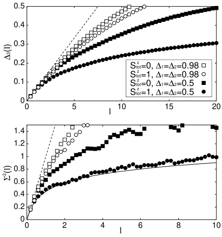
Figure 5: Spectral rigidity $\Delta_{3}(l)$ and number variance $\Sigma^{2}(l)$ of the NNN coupled chain for $L=18$, $J_{2}/J_{1}=1$, $K_{\rm tot}=0$. Broken lines, Poisson behavior; Solid lines, Wigner behavior. In each of the four distributions $P(s)$ vanishes at $s=0$: there is no degeneracy among energy levels.

The observations of the level-spacing distributions can also be confirmed by investigating spectral rigidity $\Delta_{3}(l)$ and number variance $\Sigma^{2}(l)$. In Fig. 5, $\Delta_{3}(l)$ and $\Sigma^{2}(l)$ are shown for the four cases corresponding to those of Fig. 4. For $S^{z}_{\rm tot}=1$ and $\Delta_{1}=\Delta_{2}=0.5$, Wigner behavior appears. For $S^{z}_{\rm tot}=0$ and $\Delta_{1}=\Delta_{2}=0.5$, an intermediate behavior appears, which is close to the average between Wigner and Poisson behaviors. For $\Delta_{1}=\Delta_{2}=0.98$, both for $S^{z}_{\rm tot}=0$ and $S^{z}_{\rm tot}=1$, Poisson-like behavior appears for $\Delta_{3}(l)$ and $\Sigma^{2}(l)$.

4 Integrable XXZ Spin Chain in a special case

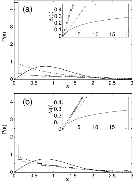
Figure 6: Level-spacing distribution $P(s)$ of the integrable chain ($J_{2}=0$) for $L=18$, $\Delta_{1}=0.5$, $S^{z}_{\rm tot}=0$, $K_{\rm tot}=2\pi/L$. (a) Desymmetrization with respect to spin reversal is not performed. (b) Desymmetrization with respect to spin reversal is performed. The inset is spectral rigidity for each case.

Let us discuss level statistics for the special case of the integrable XXZ spin chain that has the $sl_{2}$ loop algebra symmetry. Here we recall that the XXZ spin chain is integrable when the NNN coupling $J_{2}$ vanishes, and also that the $sl_{2}$ loop algebra symmetry exists when $q$ is a root of unity. Here the anisotropy $\Delta_{1}$ is related to $q$ through $\Delta_{1}=(q+q^{-1})/2$. For instance, when the parameter $q$ is given by $\exp({\rm i}\pi/3)$, we have $\Delta=0.5$.

The level spacing distribution $P(s)$ and the spectral rigidity $\Delta_{3}(l)$ of the integrable XXZ spin chain are shown for $\Delta_{1}=0.5$ in Fig. 6. In Fig. 6 (a) we do not perform the desymmetrization according to spin reversal, while in Fig. 6 (b) we plot the level-spacing distribution $P(s)$ and the spectral rigidity $\Delta_{3}(l)$ after we desymmetrize the Hamiltonian with respect to the spin reversal operation.

We observe that there still remain many degeneracies associated with the $sl_{2}$ loop algebra symmetry, even after desymmetrizing the Hamiltonian with respect to spin reversal symmetry. The level-spacing distribution $P(s)$ has a small peak at $s=0$ in Fig. 6 (b). Furthermore, the slopes of $\Delta_{3}(l)$ shown in the insets of Figs. 6 (a) and 6 (b) are larger than that of Poisson behavior. However, the numerical result does not necessarily give a counterexample to the conjecture of RMT. The level statistics might show Poisson behavior, if we completely desymmetrize the Hamiltonian matrix in terms of the $sl_{2}$ loop algebra symmetry.

5 Conclusions

For the finite spin-$\frac{1}{2}$ XXZ spin chains with the NNN interaction, we have evaluated characteristic quantities of level statistics such as the level-spacing distribution, the spectral rigidity and the number variance. Through the numerical results we have obtained the following conjecture: When the symmetry of a finite-size system enhances at some point of the parameter space, the characteristic behavior of level statistics should be given by Poisson-like behavior near some region close to the point. In particular, we have shown that finite-size effects play an important role in the characteristic quantities of level statistics for the XXZ spin chains. Here they are integrable for $J_{2}=0$, and their $U(1)$ symmetry extends into $SU(2)$ symmetry at the point of $\Delta_{1}=\Delta_{2}=1$. Furthermore, we have also shown that some unexpected non-Wigner behavior appears when an extra symmetry exists and is not considered for desymmetrization, such as the case of the spin reversal symmetry in the sector of $S^{z}_{\rm tot}=0$. Here we note that in some cases extra symmetries depend on some parameters or some quantum numbers. We have thus solved completely the observed non-Wigner behaviors of NNN coupled chain for $S^{z}_{\rm tot}=0$ in ref. NNN.

Appendix A Jordan-Wigner and Fourier Transformations

Let us rewrite eq. (3) by

$$\mathcal{H} =\mathcal{H}_{1}+\mathcal{H}_{2}$$ (8)

$$=J_{1}\sum^{L}_{l=1}(S^{x}_{l}S^{x}_{l+1}+S^{y}_{l}S^{y}_{l+1}+\Delta_{1}S^{z}_{l}S^{z}_{l+1})+J_{2}\sum^{L}_{l=1}(S^{x}_{l}S^{x}_{l+2}+S^{y}_{l}S^{y}_{l+2}+\Delta_{2}S^{z}_{l}S^{z}_{l+2}),$$

where $\mathcal{H}_{1}$ is the term containing nearest-neighbor couplings and $\mathcal{H}_{2}$ is the term containing next-nearest-neighbor couplings. We define the Jordan-Wigner transformation by

$$\sigma^{-}_{l} = \exp\left(-{\rm i}\pi\sum_{j=1}^{l-1}c_{j}^{\dagger}c_{j}\right)c_{l}^{\dagger},$$ (9)

$$\sigma^{+}_{l} = \exp\left({\rm i}\pi\sum_{j=1}^{l-1}c_{j}^{\dagger}c_{j}\right)c_{l},$$ (10)

$$\sigma^{z}_{l} = 2\sigma^{+}_{l}\sigma^{-}_{l}-1=1-2\sigma^{-}_{l}\sigma^{+}_{l},$$ (11)

where $c^{\dagger}_{j}$ and $c_{j}$ are the creation and annihilation operators of fermions on $j$th site. Under the Jordan-Wigner transformation, $\mathcal{H}_{1}$ is written by

$$\mathcal{H}_{1} = \frac{J_{1}}{4}\Delta_{1}\left(L-2\sum_{l=1}^{L}c_{l}^{\dagger}c_{l}\right)$$ (12)

$$+ \frac{J_{1}}{4}\sum_{l=1}^{L-1}[2(c_{l}^{\dagger}c_{l+1}+c_{l+1}^{\dagger}c_{l})+\Delta_{1}(4c_{l}^{\dagger}c_{l}c_{l+1}^{\dagger}c_{l+1}-2c_{l+1}^{\dagger}c_{l+1})]$$

$$+ \frac{J_{1}}{4}[2(c_{L}^{\dagger}c_{L+1}+c_{L+1}^{\dagger}c_{L})+\Delta_{1}(4c_{L}^{\dagger}c_{L}c_{L+1}^{\dagger}c_{L+1}-2c_{L+1}^{\dagger}c_{L+1})].$$

Here, we consider periodic boundary conditions ($\sigma_{L+1}^{\pm}=\sigma_{1}^{\pm}$):

$$c_{L+1} = \exp\left(-{\rm i}\pi\sum_{j=1}^{L}\sigma_{j}^{-}\sigma_{j}^{+}\right)\sigma_{L+1}^{+}=\exp\left(-\frac{{\rm i}\pi L}{2}+\frac{{\rm i}\pi}{2}\sum_{j=1}^{L}\sigma^{z}_{j}\right)\sigma_{1}^{+}$$

$$= \sigma_{1}^{+}\exp\left[{\rm i}\pi\left(-\frac{L}{2}+S^{z}_{\rm tot}+1\right)\right],$$

$$c_{L+1}^{\dagger} = \exp\left({\rm i}\pi\sum_{j=1}^{L}\sigma_{j}^{-}\sigma_{j}^{+}\right)\sigma_{L+1}^{-}=\exp\left(\frac{{\rm i}\pi L}{2}-\frac{{\rm i}\pi}{2}\sum_{j=1}^{L}\sigma^{z}_{j}\right)\sigma_{1}^{-}$$ (13)

$$= \sigma_{1}^{-}\exp\left[{\rm i}\pi\left(\frac{L}{2}-S^{z}_{\rm tot}+1\right)\right],$$

where we use ${\rm e}^{S_{1}^{z}}\sigma_{1}^{\pm}=\sigma_{1}^{\pm}{\rm e}^{S_{1}^{z}\pm 1}$. Since $\sigma_{1}^{+}=c_{1}$, $\sigma_{1}^{-}=c_{1}^{\dagger}$ , and $S^{z}_{\rm tot}=(L-M)/2-M/2=L/2-M$, where $M$ is the number of fermions, we have

$$c_{L+1}=-(-1)^{M}c_{1},\quad c_{L+1}^{\dagger}=-(-1)^{M}c_{1}^{\dagger}.$$ (14)

Therefore, $\mathcal{H}_{1}$ is rewritten as

$$\mathcal{H}_{1} = \frac{J_{1}}{4}\Delta_{1}\left[L+\sum_{l=1}^{L}+(4c_{l}^{\dagger}c_{l}c_{l+1}^{\dagger}c_{l+1}-4c_{l}^{\dagger}c_{l})\right]$$ (15)

$$+ \frac{J_{1}}{4}\cdot 2\left[\sum_{l=1}^{L-1}(c_{l}^{\dagger}c_{l+1}+c_{l+1}^{\dagger}c_{l})-(-1)^{M}(c_{L}^{\dagger}c_{1}+c_{1}^{\dagger}c_{L})\right].$$

Now, we define the Fourier transformation as

$$c_{l}={\frac{1}{\sqrt{L}}}\sum_{k}{\hat{c}}_{k}{\rm e}^{{\rm i}kl},$$ (16)

$$c_{l}^{\dagger}={\frac{1}{\sqrt{L}}}\sum_{k}{\hat{c}}_{k}^{\dagger}{\rm e}^{-{\rm i}kl}.$$ (17)

Here, $k$ takes $(2\pi/L)\times(\mbox{\rm an integer})$ for odd $M$ and $(2\pi/L)\times(\mbox{\rm a half-integer})$ for even $M$, and $0\leq k<2\pi$. After the Fourier transformation we have,

$$\mathcal{H}_{1} = \frac{J_{1}}{4}\Delta_{1}L+J_{1}\sum_{k}(\cos k-\Delta_{1}){\hat{c}}_{k}^{\dagger}{\hat{c}}_{k}$$ (18)

$$- \frac{J_{1}\Delta_{1}}{L}\sum_{k_{1},k_{2},k_{3},k_{4}}\delta_{k_{1}+k_{2},k_{3}+k_{4}}\exp\left[-{\rm i}(k_{2}-k_{4})\right]{\hat{c}}_{k_{1}}^{\dagger}{\hat{c}}_{k_{2}}^{\dagger}{\hat{c}}_{k_{3}}{\hat{c}}_{k_{4}},$$

where

$$\delta_{k_{1}+k_{2},k_{3}+k_{4}}=\left\{\begin{array}[]{ll}1&\quad\mbox{when $k_{1}+k_{2}$(mod $L$)=$k_{3}+k_{4}$(mod $L$)}.\\ 0&\quad\mbox{otherwise}.\end{array}\right.$$ (19)

Considering combination of $k$’s, we rewrite eq. (18) as

$$\mathcal{H}_{1} = J_{1}\Delta_{1}\left(\frac{L}{4}-M\right)+J_{1}\sum_{k}\cos k{\hat{c}}_{k}^{\dagger}{\hat{c}}_{k}$$ (20)

$$- \frac{2J_{1}\Delta_{1}}{L}\sum_{k_{1}<k_{2}\atop k_{3}>k_{4}}\delta_{k_{1}+k_{2},k_{3}+k_{4}}\left[\cos\left(k_{2}-k_{4}\right)-\cos\left(k_{2}-k_{3}\right)\right]{\hat{c}}_{k_{1}}^{\dagger}{\hat{c}}_{k_{2}}^{\dagger}{\hat{c}}_{k_{3}}{\hat{c}}_{k_{4}}.$$

In the same way, $\mathcal{H}_{2}$ is rewritten as

$$\mathcal{H}_{2} = J_{2}\Delta_{2}\left(\frac{L}{4}-M\right)+J_{2}\sum_{k}\cos 2k{\hat{c}}_{k}^{\dagger}{\hat{c}}_{k}$$ (21)

$$+ \frac{2J_{2}}{L}\sum_{k_{1}<k_{2}\atop k_{3}>k_{4}}\delta_{k_{1}+k_{2},k_{3}+k_{4}}\left[\cos(k_{1}+k_{3})+\cos(k_{2}+k_{4})-\cos(k_{1}+k_{4})-\cos(k_{2}+k_{3})\right]{\hat{c}}_{k_{1}}^{\dagger}{\hat{c}}_{k_{2}}^{\dagger}{\hat{c}}_{k_{3}}{\hat{c}}_{k_{4}}$$

$$- \frac{2J_{2}\Delta_{2}}{L}\sum_{k_{1}<k_{2}\atop k_{3}>k_{4}}\delta_{k_{1}+k_{2},k_{3}+k_{4}}\left\{\cos\left[2\left(k_{2}-k_{4}\right)\right]-\cos\left[2\left(k_{2}-k_{3}\right)\right]\right\}{\hat{c}}_{k_{1}}^{\dagger}{\hat{c}}_{k_{2}}^{\dagger}{\hat{c}}_{k_{3}}{\hat{c}}_{k_{4}}.$$

Appendix B Spin reversal symmetry on momentum-based fermions

Let us find the momentum-based expression of the mapping corresponding to the spin reversal transformation ($S_{j}^{\pm}\to S_{j}^{\mp}$, $S_{j}^{z}\to-S_{j}^{z}$). According to eqs. (9), (10), (16), and (17),

$${\hat{c}}_{k}=\frac{1}{\sqrt{L}}\sum_{l=1}^{L}\exp(-{\rm i}kl)\exp\left(-{\rm i}\pi\sum_{j=1}^{l-1}\sigma_{j}^{-}\sigma_{j}^{+}\right)\sigma_{l}^{+},$$ (22)

$${\hat{c}}_{k}^{\dagger}=\frac{1}{\sqrt{L}}\sum_{l=1}^{L}\exp({\rm i}kl)\exp\left({\rm i}\pi\sum_{j=1}^{l-1}\sigma_{j}^{-}\sigma_{j}^{+}\right)\sigma_{l}^{-}.$$ (23)

Under the transformation $\sigma_{l}^{\pm}\to\sigma_{l}^{\mp}$, eqs. (22) and (23) is transformed as follows.

$${\hat{c}}_{k} \to \frac{1}{\sqrt{L}}\sum_{l=1}^{L}\exp(-{\rm i}kl)\exp\left(-{\rm i}\pi\sum_{j=1}^{l-1}\sigma_{j}^{+}\sigma_{j}^{-}\right)\sigma_{l}^{-}$$ (24)

$$= \frac{1}{\sqrt{L}}\sum_{l=1}^{L}\exp(-{\rm i}kl)\exp\left[-{\rm i}\pi\sum_{j=1}^{l-1}(I_{j}-\sigma_{j}^{-}\sigma_{j}^{+})\right]\sigma_{l}^{-}$$

$$= \frac{1}{\sqrt{L}}\sum_{l=1}^{L}\exp[-{\rm i}kl-{\rm i}\pi(l-1)]\exp\left({\rm i}\pi\sum_{j=1}^{l-1}\sigma_{j}^{-}\sigma_{j}^{+}\right)\sigma_{l}^{-},$$

where $I_{j}$ is the unit matrix. Now, considering ${\rm e}^{2\pi{\rm i}l}=1$, where $l$ is an integer, we find that

$$\exp[-{\rm i}kl-{\rm i}\pi(l-1)] = \exp[-{\rm i}kl-{\rm i}\pi(l-1)+2\pi{\rm i}l]=\exp[{\rm i}(\pi-k)l+{\rm i}\pi]$$ (25)

$$= -\exp[{\rm i}(\pi-k)l].$$

Therefore, eq. (24) is rewritten as

$${\hat{c}}_{k}\to-\frac{1}{\sqrt{L}}\sum_{l=1}^{L}\exp[{\rm i}(\pi-k)l]\exp\left({\rm i}\pi\sum_{j=1}^{l-1}\sigma_{j}^{-}\sigma_{j}^{+}\right)\sigma_{l}^{-}=-{\hat{c}}_{\pi-k}^{\dagger}.$$ (26)

In the same way, we have

$${\hat{c}}_{k}^{\dagger}\to-{\hat{c}}_{\pi-k}.$$ (27)

It is sometimes convenient to use the following in stead of eqs. (26) and (27):

$${\hat{c}}_{k}^{\dagger}\to{\hat{c}}_{\pi-k},\quad{\hat{c}}_{k}\to c^{\dagger}_{\pi-k}.$$ (28)

The Hamiltonians are invariant not only for eqs. (26) and (27) but also for eq (28). The form (28) has an advantage that we do not need to consider the phase factor $-1$ that appears in eqs. (26) and (27).

Making use of the spin reversal operation expressed in terms of the fermion basis (28) we have desymmetrized the Hamiltonian matrix in the sector $S_{\rm tot}^{z}=0$ with respect to spin reversal symmetry. For a given vector with $S_{\rm tot}^{z}=0$ we calculate how it transforms under the operation (28). If it is not a singlet and transforms into a different vector, then we combine the pair into an eigenvector of the operation (28).

Similarly, when we desymmetrize the Hamiltonian with respect to parity, we use the parity operation expressed in terms of the fermion basis:

$${\hat{c}}_{k}^{\dagger}\to{\rm e}^{{\rm i}k}{\hat{c}}_{-k}^{\dagger}(-1)^{M-1+L/2-S^{z}_{\rm tot}}\,,\quad{\hat{c}}_{k}\to{\rm e}^{-{\rm i}k}{\hat{c}}_{-k}(-1)^{M+L/2-S^{z}_{\rm tot}}.$$ (29)

Here we recall that $M$ denotes the number of down-spins in the sector of $S_{\rm tot}^{z}=L/2-M$. Through the Jordan-Wigner transformation we easily derive the parity operation (29) from that on the spin variables: $\sigma_{l}^{\pm}\to\sigma_{L+1-l}^{\pm}\,,\quad\sigma_{l}^{z}\to\sigma_{L+1-l}^{z}\,$ for $l=1,2,\ldots,L$.

Appendix C Spin reversal operation on the vacuum state

When desymmetrizing the Hamiltonian with respect to spin reversal symmetry, it is useful to know how the vacuum state transforms under the spin reversal operation expressed in terms of the momentum-based fermion operators. Let us denote by $|0\rangle$ the vacuum state where there is no down-spin. Under the spin reversal operation it transforms up to a phase factor $A_{L}$ as follows

$$|0\rangle\to A_{L}\,{\hat{c}}_{q_{1}}^{\dagger}{\hat{c}}_{q_{2}}^{\dagger}\cdots{\hat{c}}_{q_{L}}^{\dagger}|0\rangle$$ (30)

Here $q_{j}$ denotes momentum $(2\pi/L)j$ for $j=1,2,\ldots,L$, when $M$ is odd, and $(2\pi/L)(j-1/2)$ for $j=1,2,\ldots,L$, when $M$ is even. The phase factor $A_{L}$ is given by

$$A_{L}={\frac{1}{L^{L/2}}}\sum_{P\in{\cal S}_{L}}\epsilon_{P}\exp(-{\rm i}\sum_{j=1}^{L}jk_{Pj})\,.$$ (31)

Here ${\cal S}_{L}$ denotes the set of permutations on $L$ elements, $\epsilon_{P}$ the sign of permutation $P$. Furthermore, we can calculate the phase factor $A_{L}$ as follows

$$A_{L}=\left\{\begin{array}[]{ccc}(-1)^{\ell}&{\rm for}&M=2\ell\\ (-1)^{\ell+1}&{\rm for}&M=2\ell+1\\ \end{array}\right.$$ (32)

The derivation is given in the following. Let us introduce the following matrix:

$$U_{s}=\prod_{j=1}^{L}\sigma_{j}^{x}\,.$$ (33)

We may express the spin reversal operation (6) as follows

$$U_{s}S^{\pm}_{j}U_{s}^{-1} = S^{\mp}_{j}\,,\quad U_{s}S^{z}_{j}U_{s}^{-1}=-S^{z}_{j}$$

$$U_{s}{\hat{c}}_{k}^{\dagger}U_{s}^{-1} = -{\hat{c}}_{\pi-k}\,,\quad U_{s}{\hat{c}}_{k}U_{s}^{-1}=-{\hat{c}}_{\pi-k}^{\dagger}.$$ (34)

We thus have

$$U_{s}\,|0\rangle=\prod_{j=1}^{L}\sigma_{j}^{x}\,|0\rangle=\sigma_{1}^{-}\sigma_{2}^{-}\cdots\sigma_{L}^{-}\,|0\rangle$$ (35)

Applying the Jordan-Wigner transformation and substituting $c_{\ell}^{\dagger}$s with ${\hat{c}}_{k}^{\dagger}$s through (17), we have

$$\sigma_{1}^{-}\sigma_{2}^{-}\cdots\sigma_{L}^{-}\,|0\rangle = c_{1}^{\dagger}c_{2}^{\dagger}\cdots c_{L}^{\dagger}|0\rangle$$ (36)

$$= {\frac{1}{L^{L/2}}}\sum_{k_{1}}\cdots\sum_{k_{L}}{\rm e}^{-{\rm i}(1k_{1}+2k_{2}+\cdots+Lk_{L})}\,{\hat{c}}_{k_{1}}^{\dagger}{\hat{c}}_{k_{2}}^{\dagger}\cdots{\hat{c}}_{k_{L}}^{\dagger}|0\rangle$$

$$= {\frac{1}{L^{L/2}}}\left(\sum_{P\in{\cal S}_{L}}{\rm e}^{(-{\rm i}\sum_{j=1}^{L}jk_{Pj})}\,\epsilon_{P}\right){\hat{c}}_{q_{1}}^{\dagger}{\hat{c}}_{q_{2}}^{\dagger}\cdots{\hat{c}}_{q_{L}}^{\dagger}|0\rangle$$

Thus we have the expression (31) of the phase factor $A_{L}$. Here we recall that $q_{j}=(2\pi/L)j$ for $j=1,2,\ldots,L$ for odd $M$, and $q_{j}=(2\pi/L)(j-1/2)$ for $j=1,2,\ldots,L$ for even $M$. We also recall that $M$ denotes the number of down-spins in the sector.

We now calculate the expression (32) for the phase factor $A_{L}$. We take a vector $|v\rangle$ with $S_{tot}^{z}=0$ as follows. When $M$ is odd, we introduce $\ell=(M-1)/2$ and we define $|v\rangle$ by

$$|v\rangle=\left({\hat{c}}_{1}^{\dagger}{\hat{c}}_{2}^{\dagger}\cdots{\hat{c}}_{\ell}^{\dagger}\right)\cdot\left({\hat{c}}_{-\ell}^{\dagger}\cdots{\hat{c}}_{-2}^{\dagger}{\hat{c}}_{-1}^{\dagger}\right)\cdot{\hat{c}}_{0}^{\dagger}|0\rangle$$

Here ${\hat{c}}_{j}^{\dagger}$ denotes ${\hat{c}}_{k}^{\dagger}$ with $k=(2\pi/L)j$. When $M$ is even, we take $\ell=M/2$, and we define $|v\rangle$ by

$$|v\rangle=\left({\hat{c}}_{1/2}^{\dagger}{\hat{c}}_{3/2}^{\dagger}\cdots{\hat{c}}_{\ell-1/2}^{\dagger}\right)\cdot\left({\hat{c}}_{-(\ell-1/2)}^{\dagger}\cdots{\hat{c}}_{-3/2}^{\dagger}{\hat{c}}_{-1/2}^{\dagger}\right)|0\rangle$$

Here ${\hat{c}}_{j+1/2}^{\dagger}$ denotes ${\hat{c}}_{k}^{\dagger}$ with $k=(2\pi/L)(j+1/2)$. Through the operation (26) we show that $U_{s}|v\rangle=(-1)^{\ell+1}A_{L}|v\rangle$ for $M$ odd and $U_{s}|v\rangle=(-1)^{\ell}A_{L}|v\rangle$ for $M$ even. Thus, we have at least $U_{s}|v\rangle=\pm|v\rangle$.

Let us show that $U_{s}|v\rangle=+|v\rangle$ for both odd $M$ and even $M$ cases. First we note that $U_{s}c_{1}^{\dagger}c_{2}^{\dagger}\cdots c_{L/2}^{\dagger}|0\rangle=c_{L/2+1}^{\dagger}c_{L/2+2}^{\dagger}\cdots c_{L}^{\dagger}|0\rangle$. Second, expanding the vector $|v\rangle$ in terms of $c_{j_{1}}^{\dagger}c_{j_{2}}^{\dagger}\cdots c_{j_{L/2}}^{\dagger}|0\rangle$ with $1\leq j_{1}<j_{2}<\cdots<j_{L/2}\leq L$, we show that the coefficient of $c_{1}^{\dagger}c_{2}^{\dagger}\cdots c_{L/2}^{\dagger}|0\rangle$ in the expansion is equal to that of $c_{L/2+1}^{\dagger}c_{L/2+2}^{\dagger}\cdots c_{L}^{\dagger}|0\rangle$. Therefore we have $U_{s}|v\rangle=+|v\rangle$.

Thus, we obtain the expression (32) for the phase factor $A_{L}$.

References

- [1] G. Montambaux, D. Poilblanc, J. Bellissard and C. Sire: Phys. Rev. Lett. 70 (1993) 497.
- [2] T. C. Hsu and J. C. Anglès d’Auriac: Phys. Rev. B 47 (1993) 14291.
- [3] D. Poilblanc, T. Ziman, J. Bellissard, F. Mila and G. Montambaux: Europhys. Lett. 22 (1993) 537.
- [4] P. van Ede van der Pals and P. Gaspard: Phys. Rev. E 49 (1994) 79.
- [5] J. C. Anglès d’Auriac and J. M. Maillard: Physica A 321 (2003) 325.
- [6] K. Kudo and T. Deguchi: Phys. Rev. B 68 (2003) 052510.
- [7] D. A. Rabson, B. N. Narozhny and A. J. Millis: Phys. Rev. B 69 (2004) 054403.
- [8] R. Berkovits and Y. Avishai: J. Phys. C 8 (1996) 389.
- [9] B. Georgeot and D. L. Shepelyansky: Phys. Rev. Lett. 81 (1998) 5129.
- [10] Y. Avishai, J. Richert and R. Berkovits: Phys. Rev. B 66 (2002) 052416.
- [11] L. F. Santos: J. Phys. A 37 (2004) 4723.
- [12] K. Kudo and T. Deguchi: Phys. Rev. B 69 (2004) 132404.
- [13] B. I. Shklovskii, B. Shapiro , B. R. Sears, P. Lambrianides and H. B. Shore: Phys. Rev. B 47 (1993) 11487.
- [14] K. Nakamura and A. R. Bishop: Phys. Rev. B 33 (1986) 1963.
-
[15]
N. Nakazono, T. Kato and K. Nakamura:
Prog. Theor. Phys. Supp. 150 (2003) 165;
S. Sawada, et al.: in preparation. - [16] T. Deguchi, K. Fabricius and B. M. McCoy: J. Stat. Phys. 102 (2001) 701.
- [17] K. Fabricius and B. M. McCoy: MathPhys Odyssey 2001, ed. M. Kashiwara and T. Miwa (Birkhäuser, Boston, 2002) p. 119.
- [18] T. Deguchi: J. Phys. A 35 (2002) 879.
- [19] D. B. Uglov and I. T. Ivanov: J. Stat. Phys. 82 (1996) 87.
- [20] M. Di Stasio and X. Zotos: Phys. Rev. Lett. 74 (1995) 2050.
- [21] H. Meyer and J. C. Anglès d’Auriac: Phys. Rev. E 55 (1997) 6608.
- [22] S. E. Nagler, W. J. L. Buyers, R. L. Armstrong and B. Briat: Phys. Rev. B 27 (1983) 1784.
- [23] S. Hirata and K. Nomura: Phys. Rev. B 61 (2000) 9453.
- [24] K. Nomura and K. Okamoto: J. Phys. A 27 (1994) 5773.
- [25] L. Urba and A. Rosengren: Phys. Rev. B 67 (2003) 104406.
- [26] It is technically difficult to desymmetrize the Hamiltonian with respect to both parity and spin reversal symmetries simultaneously.