A Study of Dynamic Finite Size Scaling Behavior of the Scaling Functions-Calculation of Dynamic Critical Index of Wolff Algorithm

SEMRA GÜNDÜÇ, MEHMET DİLAVER , MERAL AYDIN^† and YİĞİT GÜNDÜÇ

Hacettepe University, Physics Department,

06532 Beytepe, Ankara, Turkey

Abstract

In this work we have studied the dynamic scaling behavior of two scaling functions and we have shown that scaling functions obey the dynamic finite size scaling rules. Dynamic finite size scaling of scaling functions opens possibilities for a wide range of applications. As an application we have calculated the dynamic critical exponent ($z$) of Wolff’s cluster algorithm for $2$-, $3$- and $4$-dimensional Ising models. Configurations with vanishing initial magnetization are chosen in order to avoid complications due to initial magnetization. The observed dynamic finite size scaling behavior during early stages of the Monte Carlo simulation yields $z$ for Wolff’s cluster algorithm for $2$-, $3$- and $4$-dimensional Ising models with vanishing values which are consistent with the values obtained from the autocorrelations. Especially, the vanishing dynamic critical exponent we obtained for $d=3$ implies that the Wolff algorithm is more efficient in eliminating critical slowing down in Monte Carlo simulations than previously reported.

Keywords: Ising model, scaling functions, dynamic scaling, time evolution of the magnetization and the scaling functions, dynamic critical exponent.

1 Introduction

Finite size scaling and universality arguments have been used to study the critical parameters of spin systems over two decades [1]. Jansen, Schaub and Schmittmann [2] showed that for a dynamic relaxation process, in which a system is evolving according to a dynamics of Model A [3] and is quenched from a very high temperature to the critical temperature, a universal dynamic scaling behavior within the short-time regime exists [4, 5, 6]. The existence of finite size scaling even in the early stages of the Monte Carlo simulation has been tested for various spin systems [5, 6, 7, 8, 9, 10, 11, 12], the dynamic critical behavior is well-studied and it has been shown that the dynamic finite size scaling relation holds for the magnetization and for the moments of the magnetization. For the $k^{th}$ moment of the magnetization of a spin system, dynamic finite size scaling relation can be written as [2]

$$M^{(k)}(t,\epsilon,{m_{0},L})=L^{(-k{\beta}/{\nu})}{\cal{M}}^{(k)}(t/\tau,{\epsilon}L^{1/{\nu}},{m_{0}}L^{x_{0}})$$ (1)

where $L$ is the spatial size of the system, $\beta$ and $\nu$ are the well-known critical exponents, $t$ is the simulation time, ${\epsilon}=(T-{T_{c}})/{T_{c}}$ is the reduced temperature and $x_{0}$ is an independent exponent which is the anomalous dimension of the initial magnetization ($m_{0}$). In Eq.(1) $\tau$ is the autocorrelation time, $\tau\sim L^{z}$ and $z$ is the dynamic critical exponent.

 

The relation given in Eq.(1) can be used to study the known critical exponents as well as exponents $z$ and $x_{0}$. Moments of the magnetization have their own anomalous dimensions ($k{\beta}/{\nu}$) And using these quantities (in order to obtain dynamic exponents $z$ and $x_{0}$) one may expect some ambiguities due to correction to scaling and errors on determining the anomalous dimension of the given thermodynamic quantity. The ambiguities due to the anomalous dimension of the thermodynamic quantity can be avoided if one considers quantities which are themselves scaling functions. Moreover, scaling functions are extremely powerful to identify the order of the phase transition, as well as locating the transition point of statistical mechanical systems on finite lattices.

 

In this work we propose that the dynamic finite size scaling relation also holds for the scaling functions and the scaling relation can be written similarly to the moments of the magnetization,

$$O(t,\epsilon,{m_{0},L})={\cal{O}}^{(k)}(t/\tau,{\epsilon}L^{1/{\nu}},{m_{0}}L^{x_{0}})\;.$$ (2)

Our aim is to study dynamic finite size scaling behavior of the scaling functions by using Eq.(2).

 

In our calculations two different scaling functions are used. The first such quantity is Binder’s cumulant [13, 14, 15]. Binder’s cumulant is widely used in order to obtain the critical parameters as well as to determine the type of the phase transition. This quantity involves the ratio of the moments of the magnetization or energy. In this work we have used the definition of Binder’s cumulant which involves the ratio of the moments of the magnetization. Simplest such quantity can be given as

$$B_{n}=\frac{<S^{2n}>}{<S^{n}>^{2}}\;.$$ (3)

In the usual definition of Binder’s cumulant, $<S^{n}>$ is the thermal average of the $n^{\rm th}$ moment of the configuration average of the spin. In dynamic case, starting from a totally random configuration ($m_{0}=0$), runs are repeated until predetermined number of iterations are reached for each lattice size. The thermodynamic quantities are calculated as the configuration averages at each iteration. In order to calculate Binder’s cumulant iteration by iteration, the configuration averages of the magnetization and its higher moments are calculated. Various moments of the magnetization are divided iteration by iteration in order to obtain the required form of Binder’s cumulant,

$$B_{n}(t)=\frac{<S^{2n}>(t)}{<S^{n}>^{2}(t)}\;.$$ (4)

Here the averages are calculated over the configurations obtained at each iteration. In this work we use Binder’s cumulant for $n=2$ by using the the relation

$$B_{2}(t)=\frac{<S^{2}>(t)}{<|S|>^{2}(t)}\;.$$ (5)

 

The second quantity is the scaling function ($F$) based on the surface renormalization. This function is studied in detail for the Ising model [16, 17, 18] and $q$-state Potts model [19, 20, 21]. In order to calculate this function, one considers the direction of the majority of spins of two parallel surfaces which are $L/2$ distance away from each other. For Ising spins, $F$ can be written in the form [18],

$$F=<sign[{S}_{i}]sign[{S}_{i+L/2}]>$$ (6)

where $S_{i}$ is the sum of the spins in the $i^{\rm th}$ surface. Similar to the calculations of Binder’s cumulant, iteration-dependent calculation of $F$ requires the configuration averages which are obtained for each iteration yielding a Monte Carlo time dependent expression,

$$F(t)=<sign[{S}_{i}]sign[{S}_{i+L/2}]>(t)\;.$$ (7)

$F(t)$ can be used in calculating the dynamic finite size scaling relation given in Eq.(2).

 

In Wolff‘s algorithm [22], only spins belonging to a certain cluster around the seed spin are considered and updated at each Monte Carlo step. In equilibrium, the dynamic critical exponent of the Wolff’s algorithm can not be obtained directly from the observed autocorrelation times (${\tau_{W}}^{{}^{\prime}}$), instead the autocorrelation time (${\tau_{W}}$) is governed by the average size ($<C>$ of the clusters. $\tau_{W}$ can be obtained by the relation,

$$\tau_{W}\;=\;{\tau_{W}}^{{}^{\prime}}\frac{<C>}{L^{d}}\;.$$ (8)

  The dynamic critical exponents of cluster algorithms are calculated using the autocorrelation times of spin systems in thermal equilibrium [22, 23, 24, 25, 26, 27, 28]. In these studies the dynamic critical exponent is observed to be much less than the value obtained by use of local algorithms. For $2$-dimensional Ising model Wolff obtained $z\sim 0.25$ [25]. More recently, Heerman and Burkitt [26] suggested that data are consistent with a logarithmic divergence, but it is very difficult to distinguish between the logarithm and a small power [27]. For the $3$-dimensional case, Tamayo et al [28] calculated the dynamic critical exponent as $z\sim 0.44(10)$. Wolff calculated a smaller value of $z=0.28(2)$ [25] using energy autocorrelations. In $4$-dimensions, Tamayo et al [28] obtained $z$ with a vanishing value. This result is also consistent with the mean-field solution for the Ising model in four and higher dimensions. In a recent publication it has been shown that various alternative cluster algorithms posses similar dynamic behavior [29]

The efficiency of the Wolff‘s algorithm is directly related to the size of the updated clusters, hence the efficiency increases during the quenching process, as the number of iterations increases. Both the average cluster size and susceptibility have the same anomalous dimension, hence in obtaining $\tau$ from the observed behavior of the dynamic variable, one can replace $<S^{2}>$ by $<C>$. In our calculations both quantities have been used in order to scale time variable for quantities $B_{2}(t)$ and $F(t)$ considered.

2 Simulations and Results

We have studied dynamic scaling for scaling functions $B_{2}(t)$ and $F(t)$ for $2$-, $3$- and $4$-dimensional Ising models evolving in time by using Wolff’s algorithm. We have prepared lattices with vanishing initial magnetization and total random initial configurations are quenched at the corresponding infinite lattice critical temperature. We have used the lattices $L=256,384,512,640$, $L=32,48,64,80$ and $L=16,20,24$ for $2$-, $3$- and $4$-dimensional Ising models, respectively. For each lattice size, independent initial configurations are created. The number of initial configurations varies depending on the lattice size. On average, ten bins of one thousand runs, twenty bins of twenty thousand runs and ten bins of ten thousand runs have been performed for $2$- $3$-, and $4$- dimensional Ising models, respectively. Errors are calculated from the average values for each iteration obtained in different bins.

 

In the dynamic finite size scaling, for the algorithms in which all spins are checked for updating the Monte Carlo time, $t$ scales as $t/{L^{z}}$. In Wolff’s algorithm, one cluster is updated at each iteration, hence there is a need to use the average number of updated spins at each iteration. If the time is not scaled by the average cluster size, using only $L^{z}$ as a factor shifts the curves towards each other and curves cross at some point, but scaling can not be observed. In order to see a good scaling, there is a need to use a factor which is the average cluster size ($<C>(t)$) or alternatively $<S^{2}>(t)$. Dynamic scaling using $<C>(t)$ and $<S^{2}>(t)$ as the factor in time scaling results in the same value of the dynamic critical exponent $z$. The dynamic critical exponent $z$ is calculated using the relation

$$z=z^{\prime}-(2Y_{H}-d)$$ (9)

which is obtained from the relation

$$\tau=\tau{\prime}<C>$$ (10)

where $z^{\prime}$ and $\tau^{\prime}$ are the measured values of the dynamic critical exponent and the autocorrelation time. In these calculations, $Y_{H}$ is taken as $Y_{H}={15\over 8}$ (Onsager solution), $Y_{H}=2.4808$ [30, 31], $Y_{H}=3$ (mean-field solution) for the $2$-, $3$- and $4$- dimensional models, respectively. Since $<C>$ and $<S^{2}>$ scale in the same form, in our presentation we have scaled time axis with $t<S^{2}>/L^{z^{\prime}}$.

 

In Figure 1 we have presented Binder’s cumulant $(B_{2}(t))$ before and after the dynamic finite size scaling for $2$-dimensional Ising model for the lattice sizes considered. Figure 1 a) shows the time evolution of $B_{2}(t)$ during the relaxation of the system. During the relaxation process the correlation length tends to grow until it reaches the lattice size. When the correlation length approaches the lattice size, Binder’s cumulant exhibits an abrupt change and finally it settles to a new, long correlation length value. The position of this abrupt change along time axis depends on the linear size ($L$) of the lattice. But the initial and the final values are exactly the same for all lattice sizes. In Figure 1 b) the scaling of Binder’s cumulant ($B_{2}(t)$) can be seen. As it is seen from this figure, $B_{2}(t)$ scales with time as $t<S^{2}>(t)/L^{z^{\prime}}$. As a result of scaling, the value $z^{\prime}=1.725\pm 0.03$ is obtained from minimizing distances between $B_{2}(t)$ data for different lattice sizes.

 

Figure 2 shows the surface renormalization function $F(t)$ for the $2-$dimensional Ising model for the same lattice sizes given in Figure 1. Figure 2 a) shows the simulation data and Figure 2 b) shows the scaling by use of $<S^{2}>(t)$ as the factor in time scaling. This function also exhibits an abrupt change from initial vanishing value to a certain constant value as the correlation length reaches the size of the lattice. As it is seen from this figure, time to reach the plateau is proportional to the linear size $(L)$ of the system. The positions of the abrupt changes for both $F(t)$ and $B_{2}(t)$ are the same for each lattice size. As in the case of $B_{2}(t)$ given in Figure 1, a good scaling is observed for the same value of $z^{\prime}=1.725\pm 0.03$.

Figures 3 and 4 show the simulation data and the dynamic scaling for $B_{2}(t)$ and $F(t)$ for $3$- dimensional Ising model, respectively. In both figures a) shows the time evolution of the scaling functions and b) shows the functions after dynamic scaling. Scaling gives $z^{\prime}=1.95\pm 0.05$ for both $B_{2}(t)$ and $F(t)$ for the $3$-dimensional Ising model. Similarly, figures 5 and 6 show the simulation data and the dynamic scaling for $B_{2}(t)$ and $F(t)$ for $4$- dimensional Ising model, respectively. For this model scaling of data for $B_{2}(t)$ and $F(t)$ results in $z^{\prime}=2.0\pm 0.2$ and $z^{\prime}=2.1\pm 0.2$, respectively. In all these figures simulation data for functions $B_{2}(t)$ and $F(t)$ show the same behavior and scaling is very good. The errors in the values of $z^{\prime}$ are obtained from the largest fluctuations in the simulation data for $B_{2}(t)$ and $F(t)$. The values of the dynamic critical exponent $z$ are calculated using Eq.(9) for $2$-, $3$- and $4$- dimensional Ising models and these values are given in Table 1. The literature values are also given for comparison.

3 Conclusion

Wolff’s algorithm is one of the most difficult algorithms to calculate the dynamic critical exponent. Simply the difficulty arises from the comparison between the number of updated spins and the total number of spins. At each iteration only a single cluster is updated. In the literature, for $2$-, $3$- and $4$-dimensions, small dynamic critical exponents are obtained [22, 23, 24, 25, 26, 27, 28], but further studies of the data suggest that for all three dimensions the dynamic critical exponent of the Ising model can be considered as zero. The measurement of the dynamic critical exponent in thermal equilibrium is extremely difficult, since the correlation length around the phase transition point is as large as the size of the lattice. In dynamic finite size scaling, since the correlation length remains smaller than the lattice size, it is expected that statistically independent configurations lead to better statistics since there are no finite size effects.

 

In this work we have considered the dynamic scaling behavior of Binder’s cumulant ($B_{2}(t)$) and the renormalization function ($F(t)$) for $2$-, $3$- and $4$- dimensional Ising models. We have observed that these scaling functions can be used to identify the critical point and the critical exponents during the initial stages of the thermalization. In our calculations, we have observed that our results are consistent with vanishing dynamic critical exponent. Despite the fact that obtaining good statistics is extremely time consuming for large lattices, finite size effects do not play any role in obtaining the results. One can see from the results of dynamic scaling that scaling is very good and the errors are very small, hence this method is a good candidate to calculate the dynamic critical exponent for any spin model and for any algorithm. The most striking result of our calculations is that the dynamic critical exponent for $3$-dimensional Ising model is obtained as $z=0.02\pm 0.09$, instead of previously reported range of values $z=0.28-0.44$ [28, 25]. This is a clear indication that the efficiency of the Wolff’s algorithm is better than previously thought, especially in eliminating critical slowing down of Monte Carlo simulations. This means that using this algorithm, very large lattices at criticality can be considered, without unusually large statistical errors building up.

Table Captions

Table 1.

The values of calculated dynamic critical exponents ($z$) (using Eq.(9)) for $2$-, $3$- and $4$-dimensional Ising models. First two coulumns are the values obtained from scaling functions $B_{2}(t)$ and $F(t)$, respectively and the third column includes the literature values.

Figure Captions

Figure 1 a) Binder cumulant data ($B_{2}(t)$) for $2$-dimensional Ising Model for linear lattice sizes $L=256$, $384$, $512$, $640$ as a function of simulation time $t$, b) scaling of $B_{2}(t)$ data given in a) using $<S^{2}>(t)$ as the factor in time scaling,

 

Figure 2 a) Simulation data for the renormalization function ($F(t)$) as a function of simulation time $t$ for $2$-dimensional Ising model for linear lattice sizes $L=256$, $384$, $512$, $640$, b) scaling of $F(t)$ data given in a) using $<S^{2}>(t)$ as a factor in time scaling.

 

Figure 3. Simulation data for $B_{2}(t)$ as a function of simulation time $t$ for $3$-dimensional Ising model for linear lattice sizes $L=32$, $48$, $64$, $80$, b) scaling of $B_{2}(t)$ data given in a) using $<S^{2}>(t)$ as the factor in time scaling.

 

Figure 4. Simulation data for $F(t)$ as a function of simulation time $t$ for $3$-dimensional Ising model for linear lattice sizes $L=32$, $48$, $64$, $80$, b) scaling of $F(t)$ data given in a) using $<S^{2}>(t)$ as the factor in time scaling.

 

Figure 5. Simulation data for $B_{2}(t)$ as a function of simulation time $t$ for $4$-dimensional Ising model for linear lattice sizes $L=16$, $20$, $24$, b) scaling of $B_{2}(t)$ data given in a) using $<S^{2}>(t)$ as the factor in time scaling.

 

Figure 6. Simulation data for $F(t)$ as a function of simulation time $t$ for $4$-dimensional Ising model for linear lattice sizes $L=16$, $20$, $24$, b) scaling of $F(t)$ data given in a) using $<S^{2}>(t)$ as the factor in time scaling.

$~{}~{}~{}~{}~{}~{}d$	$z(B_{2})$	$z(F)$	$z(Literature)$
$~{}~{}~{}~{}~{}~{}2$	$0.0\pm 0.05$	$0.02\pm 0.05$	$0-0.4$       [25, 26, 27]
$~{}~{}~{}~{}~{}~{}3$	$0.0\pm 0.09$	$0.02\pm 0.09$	$0.28-0.44$ [28, 25]
$~{}~{}~{}~{}~{}~{}4$	$0.0\pm 0.19$	$-0.13\pm 0.19$	$0$              [28]

Table 1.

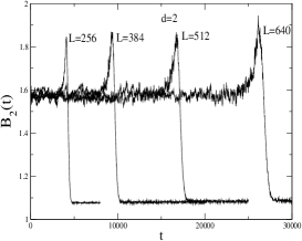
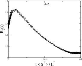
Figure 1:

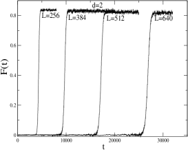
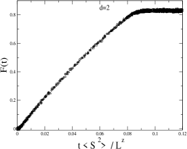
Figure 2:

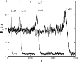
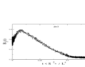
Figure 3:

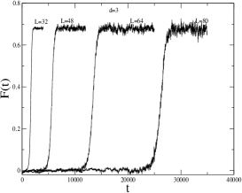
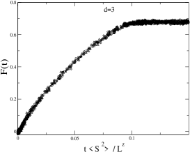
Figure 4:

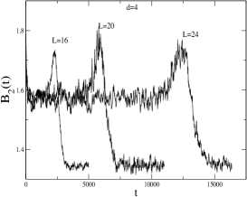
Figure 5:

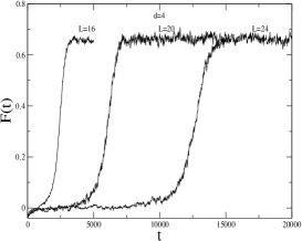
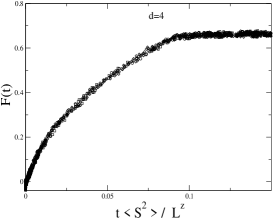
Figure 6:

References

- [1] M. N. Barber, in: Phase Transition and Critical Phenomena, eds. C. Domb and J. L. Lebowitz (Academic, New York, 1983), Vol. 8, p. 146.
- [2] H. K. Janssen, B. Schaub and B. Schmittmann, Z. Phys. B73, 539 (1989).
- [3] P. C. Hohenberg and B. I. Halperin, Rev. Mod. Phys. 49, 435 (1977).
- [4] F. G. Wang and C. K. Hu, Phys. Rev. E56, 2310 (1997).
- [5] B. Zheng, Int. J. Mod. Phys. B12, 1419 (1998).
- [6] B. Zheng, Physica A283, 80 (2000).
- [7] A. Jaster, J. Mainville, L. Schülke and B. Zheng, J. Phys. A: Math. Gen. 32, 1395 (1999).
- [8] H. J. Luo and B. Zheng, Mod. Phys. Lett. B11, 615 (1997).
- [9] H. P. Ying, B. Zheng, Y. Yu and S. Trimper, Phys. Rev. E63, R35101 (2001).
- [10] B. E. Özoğuz, Y. Gündüç and M. Aydın, Int J. Mod. Phys. C11, 553 (2000).
- [11] L. Schülke and B. Zheng, Phys. Rev. E62, 7482 (2000).
- [12] M. Dilaver, S. Gündüç, M. Aydın and Y. Gündüç, Int. J. Mod. Phys. C14, 945 (2003).
- [13] K. Binder, Phys. Rev. Lett 47, 639 (1981).
- [14] K. Binder and D. P. Landau, Phys. Rev. B30, 1477 (1984).
- [15] M. S. S. Challa, D. P. Landau and K. Binder, Phys. Rev. B34, 1841 (1986).
- [16] P. M. C. de Oliveira, Europhys. Lett. 20, (1992) 621.
- [17] P. M. C. de Oliveira, Physica A205, (1994) 101.
- [18] J. M. de F. Neto, S. M. de Oliveira, and P. M. C. de Oliveira, Physica A206, (1994) 463.
- [19] P. M. C. de Oliveira, S. M. de Oliveira, C. E. Cordeiro, and D. Stauffer, J. Stat. Phys. 80, (1995) 1433.
- [20] S. Demirtürk, N. Seferoğu, M. Aydın and Y. Gündüç, International Journal of Modern Physics C12, (2001) 403.
- [21] S. Demirtürk, Y. Gündüç, International Journal of Modern Physics C12, (2001) 1361.
- [22] U. Wolff, Phys. Rev. Lett. 62, 361 (1989).
- [23] R. H. Swendsen and J. S. Wang, Phys. Rev. Lett. 58, 86 (1987).
- [24] N. Ito and G. A. Koring, Int. J. Mod. Phys. C1, 91 (1990).
- [25] U. Wolff, Phys. Lett. B228, 379 (1989).
- [26] D. W. Heerman and A. N. Burkitt, Physica A162, 210 (1990).
- [27] C. F. Baillie and P. D. Coddington, Phys. Rev. B43, 10617 (1991).
- [28] P. Tamayo, R. C. Brower and W. Klein, J. Stat. Phys. 58, 1083 (1990).
- [29] J. -S. Wang, O. Kozan and R. H. Swendsen, Phys. Rev. E66, 057101 (2002).
- [30] H. W. J. Blöte, E. Luijten and J. R. Heringa, J. Phys. A: Math. Gen. 28, 6289 (1995).
- [31] A. L. Talapov and H. W. Blöte, J. Phys. A: Math. Gen. 29, 5727 (1996).