Domain wall effects in ferromagnet-superconductor structures.

Abstract

We investigate how domain structure of the ferromagnet in superconductor-ferromagnet heterostructures may change their transport properties. We calculate the distribution of current in the superconductor induced by magnetic field of Bloch domain walls, find the “lower critical” magnetization of the ferromagnet that provides vortices in the superconductor.

Superconductivity and ferromagnetism are two competing phenomena: while the first prefers antiparallel spin orientation of electrons in Cooper pairs, the second forces the spins to be aligned in parallel. Their coexistence in one and same material or their interaction in spatially separated materials leads to a number of new interesting phenomena, for example, $\pi$-state of superconductor (S) – ferromagnet (F) – superconductor (SFS) Josephson junctions, Ryazanov_new ; Bulaevskii ; Ryazanov ; Kontos ; Chtch_pi ; Barash ; Radovic ; Beenakker highly nonmonotonic dependence of the critical temperature $T_{c}$ of a SF bilayer as a function of the ferromagnet thickness Fominov_Ch_Golubov and so on. Recent investigations of SF bilayers showed that their transport properties often strongly depend on the interplay between magnetic structure of the ferromagnet and superconductivity. Bulaevskii_Chudnovsky ; Sonin ; Deutscher ; Kinsey ; Kadigrobov ; Pokrovsky ; Chtchelkatchev-Burmistrov ; Melin ; Ryazanov_vortices In particular, it was argued that due to ferromagnetic domains vortices may appear in the superconducting film of the SF bilayer and the domain configuration, in turn, may depend on the vortices. Pokrovsky Recently, generation of vortices by magnetic texture of the ferromagnet in SF junctions was demonstrated experimentally. Ryazanov_vortices In a number of experiments dealing with $T_{c}$ of SF bilayers, or Josephson effect in SFS structures Ryazanov_new the domain magnetizations were parallel to the SF interface. Ferromagnets used in the experiments were often dilute with the exchange field comparable to the superconducting gap and small domain size [smaller or comparable to the bulk superconductor screening length] and broad domain walls. Ryazanov_new

In this paper we try to put a step forward the answer to the question, how domain structure of the ferromagnet in SF heterostructures may change their transport properties. In the first part of the paper we discuss the junctions where S and F are weakly coupled (there is insulator layer in-between such that there is no proximity effect) and magnetizations of the domains are parallel to the SF interface. We find the distribution of current in the superconductor induced by magnetic field of the domain walls and the “lower critical” magnetization of the ferromagnet that provides vortices in the superconductor. In the end of the paper we estimate the critical temperature in strongly coupled SF bilayer when the proximity effect is strong. In this paper we do not consider the rearrangement of the domain configuration due to the superconductor Pokrovsky though we mention the superconductor induced transitions between Bloch and Neel domain wall types. The point is that the crystal structure of the ferromagnets in experiments Ryazanov_new was not perfect. Experimental data suggests that defects, dislocations in the lattice that appear during lithography process stick domain configuration.

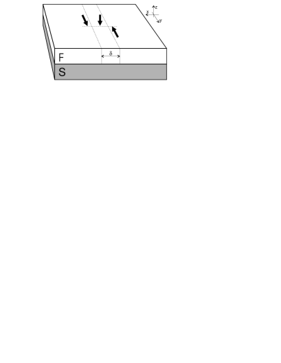
Figure 1: The SF junction. A sketch of a Bloch domain wall. The magnetization rotates according to Eq. (2). Magnetization in the center of the domain wall is perpendicular to the S film.

The domain texture of the F film is described by the following magnetization (see Fig. 1)

$$\mathbf{M}=M\theta\left(z\right)\theta\left(d_{F}-z\right)\sum\limits_{j=-\infty}^{\infty}(-1)^{j}\mathbf{m}(x-jL).$$ (1)

where vector $\mathbf{m}(x)$ rotates as follows Landau8

$$m_{x}=0,\quad m_{y}=\tanh(x/\delta),\quad m_{z}=-1/\cosh(x/\delta).$$ (2)

The vector potential $\mathbf{A}$ satisfies the Maxwell-Londons equation

$$\nabla\times(\nabla\times\mathbf{A})+\mathbf{A}\lambda_{L}^{-2}\theta\left(-z\right)\theta\left(z+d_{S}\right)=4\pi\nabla\times\mathbf{M}$$ (3)

that should be supplemented by the standard boundary conditions of continuity of $\mathbf{A}$ and $\partial\mathbf{A}/\partial z$. Landau8 By solving Eq. (3) with a help of the Fourier transformation we can find the distribution of the magnetic field $\mathbf{B}=\nabla\times\mathbf{A}$ in the entire space. BC In agreement with general expectations the $z$ component of the magnetization in the F film that collects at domain walls results in the current flow in the S film. It is convenient to define the current averaged over the thickness of the S film, $J_{y}(x)=-c/(4\pi\lambda_{L}^{2})\int_{-d_{S}}^{0}A_{y}dz$. Then we obtain

$$J_{y}(x)=-2\pi cM\frac{\delta}{\lambda_{L}^{2}L}\sum\limits_{n=0}^{\infty}\frac{\sin q_{n}x}{Q_{n}\cosh(\frac{\pi}{2}q_{n}\delta)}\frac{Q_{n}\sinh Q_{n}d_{S}+q_{n}(\cosh Q_{n}d_{S}-1)}{(Q_{n}^{2}+q^{2}_{n})\sinh Q_{n}d_{S}+2Q_{n}q_{n}\cosh Q_{n}d_{S}}\left[1-\exp(-q_{n}d_{F})\right],$$ (4)

where $c$ stands for the speed of light, $q_{n}=\pi(2n+1)/L$ and $Q_{n}=\sqrt{q_{n}^{2}+\lambda_{L}^{-2}}$. Eq. (4) constitutes one of the principal results of the present paper. It allows to compute the distribution of the current flow in the S film for a general set of parameters $d_{S}$, $d_{F}$, $\delta$, $L$ and $\lambda_{L}$. Below we shall analyze two the most interesting cases of thick ($d_{S},d_{F}\gg\lambda_{L}$) and thin ($d_{S},d_{F}\ll\lambda_{L}$) SF bilayer.

Thick SF bilayer. Eq. (4) can be drastically simplified provided $d_{S},d_{F}\gg\lambda_{L}$ such that the current $J_{y}(x)$ becomes independent on the widths $d_{S}$ and $d_{F}$ of the S and F films. It is given as

$$J_{y}(x)=-cM\frac{2\pi\delta}{\lambda_{L}^{2}L}\sum\limits_{n=0}^{\infty}\frac{\sin q_{n}x}{\cosh\frac{\pi}{2}q_{n}\delta}\frac{1}{Q_{n}(Q_{n}+q_{n})}.$$ (5)

In order to understand the distribution of the current $J_{y}(x)$ as determined by Eq. (5) we shall first analyze the case of a single domain wall. Taking the limit $L\to\infty$ in Eq. (5), we obtain the following result for the current in the presence of a single domain wall in the F film

$$\frac{J_{y}(x)}{cM}=-\frac{\delta}{\lambda_{L}}\int_{0}^{\infty}\frac{d\omega}{\sqrt{1+\omega^{2}}}\frac{\sin\frac{x}{\lambda_{L}}\omega}{\cosh\frac{\pi\omega\delta}{2\lambda_{L}}}\frac{1}{\omega+\sqrt{1+\omega^{2}}}.$$ (6)

The distribution of the current $J_{y}(x)$ is governed by the single parameter $\pi\delta/(2\lambda_{L})$ as it is shown in Fig. 2. If the width $\delta$ of the domain wall is small compared to the Londons penetration length $\lambda_{L}$, $\pi\delta/(2\lambda_{L})\ll 1$, we find the distribution of the current as

$$J_{y}(x)=cM\begin{cases}\frac{\delta}{x}\left[\frac{|x|}{\lambda_{L}}K_{1}\left(\frac{|x|}{\lambda_{L}}\right)-1\right],&|x|\gg\delta,\\ \frac{x\delta}{2\lambda_{L}^{2}}\ln\frac{\pi\delta}{2\lambda_{L}},&|x|\ll\delta,\end{cases}$$ (7)

where $K_{1}(x)$ is the modified Bessel function of the second kind. In the opposite case of the thick domain wall, $\pi\delta/(2\lambda_{L})\gg 1$, we obtain

$$\frac{J_{y}(x)}{cM}=\tanh\frac{x}{\delta}-\frac{2}{\pi}\mathop{\mathrm{missing}}{Im}\nolimits\psi\left(\frac{1}{4}+i\frac{x}{2\pi\delta}\right)+\frac{\lambda_{L}}{\delta}\frac{\tanh\frac{x}{\delta}}{\cosh\frac{x}{\delta}},$$ (8)

where $\psi(x)$ denotes the digamma function.

According to Eqs. (7) and (8) the current $J_{y}(x)$ behaves linearly with $x$ for $x\ll\delta$ and decays as a power law for large $x$. The current distribution $J_{y}(x)$ is spread on the length $L_{s}\propto\max\{\delta,\lambda_{L}\}$ from the origin whereas its maximal value $J_{y}^{m}\propto cM\delta/L_{s}=cM\min\{1,\delta/\lambda_{L}\}$.

Now we turn back to the general case of multi domain wall structure in the F film that corresponds to a finite size $L$ of domains. We have evaluated the sum in Eq. (5) numerically and present results for the current distribution in Fig. 3. While $\lambda_{L}$ remains small compared with $L$ the profile of $J_{y}(x)$ corresponds to almost independent current distributions near each domain wall that results in distinctive two maximum structure as shown in Fig. 3. When $\lambda_{L}$ becomes of the order of $L$ the two maximum structure transforms into sinusoidal profile with the maximum exactly in the middle of a domain.

Thin SF bilayer. In the case of the thin SF bilayer, $d_{S},d_{F}\ll\lambda_{L}$, by expanding the general expression (4) in powers of $d_{S}$ and $d_{F}$, we find

$$J_{y}(x)=-cMd_{F}\frac{2\pi\delta}{L}\sum\limits_{n=0}^{\infty}\frac{\sin q_{n}x}{\cosh\frac{\pi}{2}q_{n}\delta}\frac{q_{n}}{1+2q_{n}\lambda}.$$ (9)

Here $\lambda=\lambda_{L}^{2}/d_{S}$ usually referred as the effective penetration length. Pearl We shall first analyze the case of a single domain wall again. In the limit $L\to\infty$ we obtain from Eq. (9)

$$J_{y}(x)=-cM\frac{d_{F}\delta}{4\lambda^{2}}\int_{0}^{\infty}d\omega\frac{\omega}{1+\omega}\frac{\sin\frac{x}{2\lambda}\omega}{\cosh\frac{\pi\delta}{4\lambda}\omega}.$$ (10)

The distribution of the current $J_{y}(x)$ is presented in Fig. 4 for different values of the parameter $\pi\delta/(4\lambda)$.

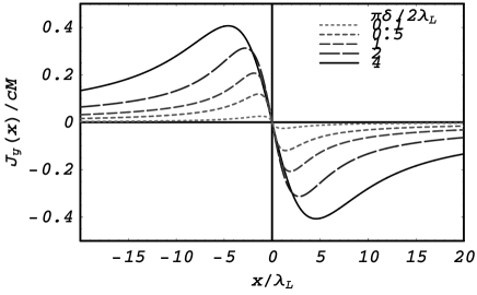
Figure 2: The case $d\gg\lambda_{L}$. The plot of $J_{y}(x)/(cM)$ as a function of $x/\lambda_{L}$ for $\pi\delta/(2\lambda_{L})=0.1,0.5,1,2,4$.

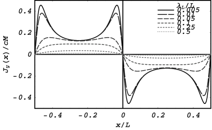
Figure 3: The case $d\gg\lambda_{L}$. The plot of $J_{y}(x)/(cM)$ as a function of $x/L$ for $\delta/L=0.02$ and $\lambda_{L}/L=0.005,0.01,0.05,0.1,0.25,0.5$.

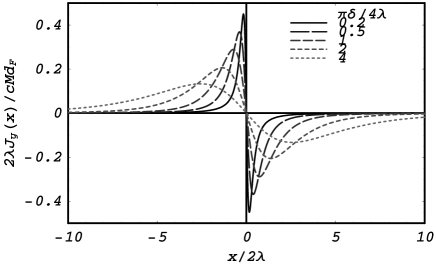
Figure 4: The case $d\ll\lambda_{L}$. The plot of $2\lambda J_{y}(x)/(cMd_{F})$ as a function of $x/(2\lambda)$ for $\pi\delta/(4\lambda)=0.2,0.5,1,2,4$.

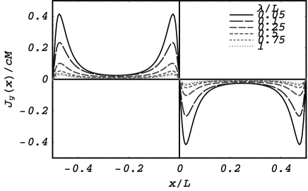
Figure 5: The case $d\ll\lambda_{L}$. The plot of $J_{y}(x)/(cM)$ as a function of $x/L$ for $\delta/L=0.02$, $d_{F}/L=0.1$ and $\lambda/L=0.05,0.1,0.25,0.5,0.75,1$.

If the domain wall is thin, $\pi\delta/(4\lambda)\ll 1$, Eq. (10) yields

$$\frac{J_{y}(x)}{cM}=\frac{d_{F}}{2\lambda}\Bigl{[}\tanh\frac{x}{\delta}-\frac{2}{\pi}\mathop{\mathrm{missing}}{Im}\nolimits\psi\left(\frac{1}{4}+i\frac{x}{2\pi\delta}\right)+\frac{\delta}{2\lambda}g(x)\Bigr{]},$$ (11)

where

$$g(x)=\begin{cases}\frac{\pi}{2}\operatorname{sign}x\cos\frac{x}{2\lambda}+f(\frac{x}{2\lambda}),&|x|\gg\delta,\\ \frac{x}{\delta},&|x|\ll\delta.\end{cases}$$ (12)

Here $f(x)=\sin x\mathop{\rm ci}\nolimits(x)-\cos x\mathop{\rm si}\nolimits(x)$ with $\mathop{\rm ci}\nolimits(x)$ and $\mathop{\rm si}\nolimits(x)$ being the cosine and sine integral functions. In the opposite case $\pi\delta/(4\lambda)\gg 1$ the current distribution $J_{y}(x)$ is given as

$$\frac{J_{y}(x)}{cM}=-\frac{d_{F}}{\delta}\frac{\tanh x/\delta}{\cosh x/\delta}.$$ (13)

Eqs. (11) and (13) proves that the $J_{y}(x)$ increases linearly with $x$ for $x\ll\delta$ and decreases algebraically for large $x$. The position of the maximum of $J_{y}(x)$ is situated at $L_{s}\propto\delta$ and the value at the maximum $J_{y}^{m}\propto(d_{F}/\delta)\min\{1,\delta/\lambda\}$. As one can see therefore the current distribution for the thin SF bilayer is qualitatively different from one for the thick SF bilayer.

In the case of multi domain wall structure in the F layer we have performed evaluation of the sum in Eq. (9) numerically and have obtained the results for the current distribution $J_{y}(x)$ presented in Fig. 5. We mention that the two maximum structure survives even for $\lambda$ of the order of $L$ for the thin SF bilayer.

As known the lower critical field for a thin S film is much smaller than for the bulk superconductor. Therefore it is possible that even small magnetization collects at domain walls can induce a vortex in the thin S film. Pokrovsky Let us assume that there is a single vortex in the the thin S film situated at $x=0$. The magnetic field becomes a sum of the magnetic field induced by the domain walls and the magnetic field of the vortex. The free energy can be written as

$$F=\int d^{3}\mathbf{r}\left(\frac{\mathbf{B}^{2}}{8\pi}+\frac{\lambda^{2}}{8\pi}|\nabla\times\mathbf{B}|^{2}-\mathbf{M}\mathbf{B}\right),$$ (14)

where $\mathbf{B}$ denotes the total magnetic field. The difference $\mathcal{F}$ of the free energy for the state with the vortex and the free energy for the state without vortex is given as follows BC

$$\mathcal{F}=\frac{\phi_{0}}{4\pi}H_{c_{1}}\lambda\left[1-\frac{M}{M_{c}}\right],\,\,\,M_{c}=\frac{H_{c_{1}}}{4\pi}\frac{\lambda}{d_{F}}\mathcal{G}(\delta,\lambda,L),$$ (15)

where $\phi_{0}=ch/(2e)$, $H_{c_{1}}=(\phi_{0}/4\pi\lambda^{2})\ln\lambda/\xi$ is the lower critical field in the thin S film without the F film and

$$\mathcal{G}(\delta,\lambda,L)=\left[\frac{2\pi}{L}\sum\limits_{n=0}^{\infty}\frac{1}{\cosh\frac{\pi q_{n}\delta}{2}}\frac{\delta}{(1+2q_{n}\lambda)^{2}}\right]^{-1}.$$ (16)

The $\mathcal{F}$ becomes negative if $M>M_{c}$ and vortices can proliferate in the S film until vortex-vortex interaction stops it or (that is more probable) the domain wall changes to Neel domain wall type to reduce the free energy. In the most interesting case of a single domain wall we find

$$M_{c}=\frac{H_{c_{1}}}{4\pi}\frac{\lambda}{d_{F}}\begin{cases}2\lambda/\delta,&\pi\delta/4\lambda\ll 1,\\ 1-32G\lambda/(\pi^{2}\delta),&\pi\delta/4\lambda\gg 1,\end{cases}$$ (17)

where $G\approx 0.916$ stands for the Catalan constant. (Note, that $M_{c}$ given by Eq.(17) differs from estimates of Ref.Pokrovsky, ).

In conclusion, domain wall effects in ferromaget-superconductor structures are investigated. We find the distribution of current in the superconductor induced by magnetic field of Bloch domain walls, calculate the “lower critical” magnetization of the ferromagnet that provides vortices in the superconductor.

We neglected above the proximity effect in SF structure assuming that the ferromagnet and the superconductor are weakly coupled. Below we discuss the case when S and F are strongly coupled. Consider a SF bilayer with a perfect SF boundary. When the superconductor and the ferromagnet are thin enough then the bilayer can be described as a “ferromagnetic superconductor” with effective parameters:Bergeret-Efetov the superconducting gap $\Delta_{\rm eff}$, the exchange field $E_{\rm ex}^{(\rm eff)}$… The superconductivity survives in this system until $E_{\rm ex}^{(\rm eff)}<\Delta_{\rm eff}^{(0)}$, where $\Delta_{\rm eff}^{(0)}$ is the gap at $E_{\rm ex}^{(\rm eff)}=0$.Bergeret-Efetov Domain wall structure of the ferromagnet makes the effective exchange field nonhomogeneous. We find that if $E_{\rm ex}^{(\rm eff)}$ changes its sign on scales of the order of $\xi_{0}$ or smaller then superconductivity in the bilayer survives at $\sqrt{\langle(E_{\rm ex}^{(\rm eff)})^{2}\rangle}>\Delta_{\rm eff}^{(0)}$, where $\langle(E_{\rm ex}^{(\rm eff)})^{2}\rangle$ is the average square of the effective exchange field over the sample.Chtchelkatchev-Burmistrov

We are grateful to V. Ryazanov for stimulating discussions and also thank RFBR  Project No. 03-02-16677, 04-02-08159 and 02-02-16622, the Russian Ministry of Science, the Netherlands Organization for Scientific Research  NWO, CRDF, Russian Science Support foundation and State Scientist Support foundation (Project No. 4611.2004.2).

References

- (1) For review see V. V. Ryazanov, V. A. Oboznov, A.S. Prokofiev et al, J. Of Low Temp. Phys. 136, 385 (2004).
- (2) L. N. Bulaevskii, V. V. Kuzii, and A. A. Sobyanin, JETP Lett. 25, 290 (1977); A. V. Andreev, A. I. Buzdin, and R. M. Osgood, Phys. Rev. B 43, 10124 (1991); A. I. Buzdin, B. Vujicic, and M. Yu. Kupriyanov, Zh. Eksp. Teor. Fiz. 101, 231 (1992) [Sov. Phys. JETP 74, 124 (1992)].
- (3) A. V. Veretennikov, V. V. Ryazanov, V. A. Oboznov et al., Physica B 284-288, 495 (2000); V. V. Ryazanov, V. A. Oboznov, A. Yu. Rusanov et al., Phys. Rev. Lett. 86, 2427 (2001).
- (4) T. Kontos, M. Aprili, J. Lesueur, et al, Phys. Rev. Lett. 89, 137007 (2002).
- (5) N.M. Chtchelkatchev, W. Belzig, Yu.V. Nazarov, and C. Bruder, JETP Lett. 74, 323 (2001); N.M. Chtchelkatchev, Pis’ma v ZhETF vol.80, iss.12, pp.875-879(2004).
- (6) Yu. S. Barash and I. V. Bobkova, Phys. Rev. B 65, 144502 (2002).
- (7) M. Bozovic, and Z. Radovic, Phys. Rev. B 66, 134524 (2002); Z. Radovic, N. Lazarides, and N. Flytzanis, Phys. Rev. B 68, 014501 (2003).
- (8) C.W.J. Beenakker, Phys. Rev. Lett. 67, 3836 (1991).
- (9) Ya.V. Fominov, N.M. Chtchelkatchev, and A.A. Golubov, JETP Lett. 74, 96 (2001).
- (10) L.N. Bulaevskii and E.M. Chudnovsky, Phys. Rev. B 63, 012502 (2000).
- (11) E.B. Sonin, Phys. Rev. B 66, R100504 (2002).
- (12) S. Erdin, A.F. Kayali, I. F. Lyuksyutov, and V. L.Pokrovsky, Phys. Rev. B 66, 014414 (2002); V.L. Pokrovsky and H. Wei, Phys.Rev. B 69, 104530 (2004); Luksyitov and V.L Pokrovsky, Mod. Phys. Lett. 14, 409 (2000).
- (13) G. Deutscher and D. Feinberg, Appl. Phys. Lett. 76, 487; R. Melin, J. Phys.: Condens. Matter 13, 6445 (2001).
- (14) R.J. Kinsey, G. Burnell, and M.J. Blamir, IEEE Trans. Appl. Superc. 11, 904 (2001).
- (15) A. Kadigrobov, R.I. Shekhter, and M. Jonson, Europhys. Lett. 54, 394 (2001); F.S. Bergeret, A.F. Volkov, and K.B. Efetov, Phys. Rev. Lett. 86, 4096 (2001).
- (16) N.M. Chtchelkatchev and I.S. Burmistrov, Phys. Rev. B 68, R140501 (2003).
- (17) R. Melin, and S. Peysson, Phys. Rev. B 68, 174515 (2003).
- (18) V. V. Ryazanov et al., JETP Lett. 77, 39 (2003).
- (19) L.D. Landau and E.M. Lifshitz, in Course in Theoretical Physics, Vol. 8 (Pergamon Press, Oxford, 1984).
- (20) I.S. Burmistrov and N.M. Chtchelkatchev, in preparation.
- (21) J. Pearl, J. Appl. Phys. Lett. 5, 65 (1964).
- (22) F. S. Bergeret, A. F. Volkov, and K. B. Efetov, Phys. Rev. Lett. 86, 3140 (2001); Phys. Rev. B 64, 134506 (2001).