Kinetics of growth process controlled by mass-convective fluctuations and finite-size curvature effects

Abstract

In this study, a comprehensive view of a model crystal formation in a complex fluctuating medium is presented. The model incorporates Gaussian curvature effects at the crystal boundary as well as the possibility for superdiffusive motion near the crystal surface. A special emphasis is put on the finite-size effect of the building blocks (macroions, or the aggregates of macroions) constituting the crystal. From it an integrated static-dynamic picture of the crystal formation in terms of mesoscopic nonequilibrium thermodynamics (MNET), and with inclusion of the physically sound effects mentioned, emerges. Its quantitative measure appears to be the overall diffusion function of the formation which contains both finite-size curvature-inducing effects as well as a time-dependent superdiffusive part. A quite remarkable agreement with experiments, mostly those concerning investigations of dynamic growth layer of (poly)crystaline aggregation, exemplified by non-Kossel crystals and biomolecular spherulites, has been achieved.

PACS numbers: 05.20.Dd, 05.40.-a, 05.60.Cd, 05.70.Ln, 05.70.Np, 05.10.Gg, 61.46.+w, 61.50.Ah

1 Introduction

The present study is devoted to modeling a formation of a soft (ordered) material known as the non–Kossel crystal [1], as well as to propose how to model a polycrystalline aggregate termed the soft-matter spherulite [2]. The approach we are exploring throughout this paper assumes that the system of interest is a mesoscopic system [3], by its nature combining both classical and quantum-mechanical properties, though we are offering here a description based on nonequilibrium statistical thermodynamics, taken suitably at a mesoscopic (molecular cluster) level [4], i.e. a classical limit of the approach can preferentially be exploited [5].

In general, examples of soft materials include biopolymers and charged polymer solutions, protein/membrane complexes, colloidal suspensions, gels, nucleic acids and their assemblies, to mention but a few. Most forms of condensed matter - except of metals and ceramics (perhaps) [6] - are soft and these substances are composed of aggregates and macromolecules, with interactions that are too weak and complex to form crystals spontaneously; therefore, the task of how to grow crystals in complex environments still remains a real challenge [7].

Thus, the phrase ’soft condensed matter’ has been coined, also for the clear reasons mentioned below. First, a striking feature is that slight perturbations in temperature, pressure or concentration, or small (piconewton) external forces, can all be enough to essentially induce microstructural changes. Second, thermal fluctuations are almost by definition pronounced in soft materials, and in consequence, entropy is a privileged determinant of a soft microstructure formation, so that disorder, slow dynamics and kinetics, and plastic deformation are the rules [8]. Although soft materials have attracted engineers for ages, only recently have physicists taken an interest in such materials, and attempted to implement what is the essence of physics, that is to produce, at various levels of description, simple models that include the possible minimum information required to explain relevant features, cf. an example concerning proteins [9].

Nowadays, especially with the advent of single molecule spectroscopies are we managing to get quantitative data on things such as aggregation (and folding) effects in complex biomolecular environments, motion of molecular motors [10], electron and proton transfer rates [11], etc., that are sufficiently reliable to formulate and test simple models. The availability of new experimental tools and simulation capability are urging physicists to apply their methods to structural biology, i.e. to allow the prediction of structure on the basis of known microscopic forces.

A key issue is the fact that the environments in which a formation of the soft material happens are characteristic of pronounced spatial variations in dielectric constant, e.g. water and lipids [12]. It is of major importance to realize that competition between interactions of different ranges results in different types of aggregation of molecules. The starting point should thus be about a discussion of the relative role of the various fundamental interactions in such systems (electrostatic, hydrophobic, conformational, steric, van der Waals, etc.), and what is their real impact on the aggregation of possibly ordered (crystal formation) and/or disordered types. The next focus could be on how these competing interactions influence the form (and, topology) of soft and biological matter, like biopolymers and proteins, leading to self-assembling systems of the type listed above [13].

In the underlying study, let us propose a way of modeling the soft matter objects named non–Kossel crystals [7], and in part also the biopolymeric spheroidal polycrystals, commonly termed spherulites. The way that we have chosen to achieve the above stated goal is based on the assumption that the biomolecular system, generally out of equilibrium, can be best described at a mesoscopic level, using the conception of mesoscopic nonequilibrium thermodynamics (MNET) [14], section 2. In sections 3 and 4, we will offer the thermodynamic-kinetic description of the soft material formation first by introducing its deterministic part (section 3), and second, by going to its stochastic, no doubt, more interesting part (section 4). In the deterministic part, we wish to place our emphasis on an unquestionable basis of each soft material formation, namely, how does the material formation depend upon the boundary effect, being typically curvature-dependent, and having also - in the case of spherulites - a nonequilibrium kinetic account readily involved in the overall process. In the stochastic part, in turn, we are lucky to support our mesoscopic view by a microscopic picture of a sub-process, essentially limiting the model material formation in the crystal boundary layer [15]. Here, we have in mind the physical fact that the growth of the objects that we model can thoroughly be controlled by the macroion velocity field of the crystal ambient phase nearby its interface with the growing crystal. Since it may lead to some very interesting physical consequences, e.g. a time-dependent viscosity effect [16] (section 4), we are going to exploit this experimentally justified observation [17] in a sufficient detail, looking at the macroion finite-size effect (FSE), and its impact on the overall crystallization process seen as a combination of static (curvature-oriented) and dynamic (constrained motion-oriented) effects in the crystal’s growth layer [15]. Concluding address, contained in section 5, closes the paper.

2 MNET and its application to nucleation and growth phenomena

Mesoscopic nonequilibrium thermodynamics (MNET) provides a general framework from which one can study the dynamics of systems defined at the mesoscale [14, 18], and has been applied to analyze different irreversible processes taking place at those scales [4]. The formulation of the theory is based on the fact that a reduction of the observational time and length scales of a system usually entails an increase in the number of degrees of freedom which have not yet equilibrated and that therefore exert an influence on the overall dynamics of the system. Those degrees of freedom $\gamma$ ($\equiv\{\gamma_{i}\}$) may for example represent the velocity of a particle, the orientation of a spin, the size of a macromolecule or any coordinate or order parameter whose values properly define the state of a mesoscopic system in a phase space. The characterization of the state of the system essentially relies on the knowledge of $P(\gamma,t),$ the probability density of finding the system at the state $\gamma\in(\gamma,\gamma+d\gamma)$ at time $t.$ One can then formulate the Gibbs entropy postulate [8, 19] in the form

$$S=S_{eq}-k_{B}\int P(\gamma,t)\ln\frac{P(\gamma,t)}{P_{eq}(\gamma)}d\gamma\;.$$ (1)

Here $S_{eq}$ is the entropy of the system when the degrees of freedom $\gamma$ are at equilibrium. If they are not, the contribution to the entropy arises from deviations of the probability density $P(\gamma,t)$ from its equilibrium value $P_{eq}(\gamma)$ given by

$$P_{eq}(\gamma)\sim\exp\left(\frac{-\Delta{\cal W}(\gamma)}{k_{B}T}\right),$$ (2)

where $\Delta{\cal W}\equiv\Delta{\cal W}(\gamma)$ is the minimum reversible work required to create that state [20], $k_{B}$ is Boltzmann’s constant, and $T$ is the temperature of the heat bath. Variations of the minimum work for a thermodynamic system are expressed as

$$\Delta{\cal W}=\Delta E-T\Delta S+p\Delta V-\mu\Delta M+\sigma\Delta\Sigma+\ldots\,,$$ (3)

where (using a standard notation) extensive quantities refer to the system and intensive ones to the bath. The last term represents the work performed on the system to modify its surface $\Sigma$, whereas $\sigma$ stands for the surface tension.

To obtain the dynamics of the mesoscopic degrees of freedom one first takes variations in Eq. (1)

$$\delta S=-k_{B}\int\delta P(\gamma,t)\ln\frac{P(\gamma,t)}{P_{eq}(\gamma)}\,d\gamma.$$ (4)

focusing only on the nonequilibrated degrees of freedom.

The probability density evolves in the $\gamma-$space according with the continuity equation

$$\frac{\partial P(\gamma,t)}{\partial t}=-\frac{\partial J(\gamma,t)}{\partial\gamma},$$ (5)

where $J(\gamma,t)$ is an unknown probability current. To obtain its value, one proceeds to derive the expression of the entropy change, $dS/dt$, which follows from the continuity equation (5) and the Gibbs equation (4). After a partial integration, one then arrives at

$$\frac{dS}{dt}=-\int\frac{\partial}{\partial\gamma}J_{S}d\gamma+\sigma_{e},$$ (6)

where $J_{S}=J(\gamma,t)ln\frac{P(\gamma,t)}{P_{eq}(\gamma)}$ is the entropy flux, and

$$\sigma_{e}=-k_{B}\,\int J(\gamma,t)\,\frac{\partial}{\partial\gamma}\left(\ln\frac{P(\gamma,t)}{P_{eq}(\gamma)}\right)\,d\gamma,$$ (7)

is the entropy production which is expressed in terms of currents and conjugated thermodynamic forces defined in the space of mesoscopic variables. We will now assume a linear dependency between fluxes and forces and establish a linear relationship between them

$$J(\gamma,t)=-k_{B}L(\gamma)\,\frac{\partial}{\partial\gamma}\left(\ln\frac{P(\gamma,t)}{P_{eq}(\gamma)}\right),$$ (8)

where $L\equiv L(\gamma)$ is an Onsager coefficient, which depends on the mesoscopic coordinates $\gamma$; in general, it also depends on the state variable $P(\gamma,t)$. To derive this expression, locality in $\gamma-$space has also been taken into account, for which only fluxes and forces with the same value of $\gamma$ become coupled.

The resulting kinetic equation then follows by substituting Eq. (8) back into the continuity equation (5)

$$\frac{\partial P(\gamma,t)}{\partial t}=\frac{\partial}{\partial\gamma}\left(D(\gamma,t)P(\gamma,t)\frac{\partial}{\partial\gamma}ln\frac{P(\gamma,t)}{P_{eq}(\gamma)}\right),$$ (9)

where we have defined the diffusion coefficient as $D(\gamma,t)\equiv\frac{k_{B}L(\gamma)}{P(\gamma,t)}$. This equation, which in view of Eq. (2) can also be written as

$$\frac{\partial P(\gamma,t)}{\partial t}=\frac{\partial}{\partial\gamma}\left(D(\gamma,t)\frac{\partial P(\gamma,t)}{\partial\gamma}+\frac{D(\gamma,t)}{k_{B}T}\frac{\partial\Delta{\cal W}}{\partial\gamma}P(\gamma,t)\right)\,,$$ (10)

is the Fokker-Planck equation accounting for the evolution of the probability density in $\gamma$-space.

2.1 Nucleation processes

The expression of the nucleation rates can be obtained from the proposed formalism [5]. To this purpose one has to interpret the nucleation (or in general any activated process) as a diffusion process along the mesoscopic coordinate describing the state of the system, the embryos, at short time scales in between the metastable and the crystal phases. The reaction rate or diffusion current can be written in terms of the fugacity $z\equiv\exp\mu/k_{B}T$ as

$$J(\gamma,t)=-k_{B}L\frac{1}{z}\frac{\partial z}{\partial\gamma}.$$ (11)

The current can also be expressed as

$$J(\gamma,t)=-D(\gamma,t)\frac{\partial z}{\partial\gamma},$$ (12)

where $D(\gamma,t)=k_{B}L/z$ represents the diffusion coefficient. As a first approximation we assume that $D(\gamma,t)=D=const.$ and integrate from the initial to the final position, obtaining

$$\overline{J}\equiv\int_{\mu_{1}}^{\mu_{2}}Jd\gamma=-D(z_{2}-z_{1})=-D(\exp\frac{\mu_{2}}{k_{B}T}-\exp\frac{\mu_{1}}{k_{B}T}).$$ (13)

This equation can alternatively be expressed as

$$\overline{J}=J_{0}\left(1-e^{A/k_{B}T}\right),$$ (14)

where $\overline{J}$ is the integrated rate, $J_{0}=Dexp(\mu_{1}/k_{B}T)$ and $A=\mu_{1}-\mu_{2}$ is the affinity. We have then shown that a mesoscopic thermodynamic analysis may lead to the formulation of the nonlinear kinetic laws governing nucleation processes. Nucleation processes in which the embryos are embedded in an inhomogeneous bath can also be studied by means of the theory proposed [5].

2.2 Agglomeration and growth processes

MNET can in general be used to study kinetic processes taking place in mesostructures such as the nanostructure arrays [21]. The size of these structures is in between those of single particles and macroscopic objects. They carry out assembling (clustering) and impingement (pattern formation) processes. They may also diffuse in a thermal bath, be convected by external flow and be affected by external driving forces as those acting in extrusion, shearing, injection processes involved in the mechanical processing of a melt. The growth rate of the agglomerates can be determined by the formalism previously presented in which the mesoscopic variable is the volume of the grain. One formulates the Gibbs entropy postulate in terms of the probability density $P(\mathrm{v},t)$, where now the degree of freedom $\gamma$ is $\mathrm{v}$ - the volume of the grain or molecular cluster. Proceeding as indicated previously one obtains the growth rate

$$J(\mathrm{v},t)=\frac{L(\mathrm{v})}{TP(\mathrm{v},t)}\left[k_{B}T\frac{\partial P(\mathrm{v},t)}{\partial\mathrm{v}}+P(\mathrm{v},t)\frac{\partial\Phi}{\partial\mathrm{v}}\right]$$ (15)

Interpreting $\Phi$ as an entropic potential [22] and assuming that the volume-dependent Onsager coefficient $L(\mathrm{v})$ follows a power law of the type $\mathrm{v}^{\delta}$, where $\delta=1-1/d$, with $d$ the dimension of the system, one obtains the expression of the rate [18, 22]

$$J(\mathrm{v},t)=-\sigma_{a}\mathrm{v}^{\delta-1}P(\mathrm{v},t)-D_{a}\mathrm{v}^{\delta}\frac{\partial P(\mathrm{v},t)}{\partial\mathrm{v}}$$ (16)

where $\sigma_{a}$ and $D_{a}$ are reference constants [18]. This expression constitutes the Louat–Mulheran–Harding ($L-M-H$) law [23] proposed heuristically by assuming that the drift is due to surface tension effects, considering only the mean curvature. The procedure can be generalized to the case in which the Gaussian curvature is important which occurs at small sizes of the grains [22].

In the offered modeling we would explore another degree of freedom which is $R$, the radius of a molecular cluster or a crystal. It appears naturally in the modeling being of the form of Fokker-Planck type [1].

2.3 An example: $2D$ modeling of a crystal growth in complex environment and its MNET features

A multigrain growth has also been considered as a discretized process in terms of MNET in both space and time domains [6]. The model is mesoscopic in the sense that each cell can contain (i) a liquid unit of phase ${\sc l}$, (ii) a crystal unit, (iii) a small particle embedded in some melt or (iv) a solid large particle. Initially, each cell of the lattice contains either a large particle with some probability $P_{l}$, or a small particle embedded in some liquid ${\sc l}$ with a probability $P_{s}$, or a liquid unit with a probability $1-{P_{l}}-{P_{s}}$. Nucleation is induced by simultaneously turning a number $n$ of cells into initial solid units, supposed to be randomly dispersed in the initial melt. Since the process occurs over long time scales, thermodynamic (i.e. equilibrium-like) quantities can be mapped into multigrain growth probability rules, as follows. At each growth step, all $i$ cells containing some liquid phase, i.e. ${\sc l}$-cells and cells with a small particle, in contact with mesoscopic cells are selected. The probability $P_{i}$ to grow the phase on the cell $i$ is given by a classical thermodynamic argument as $P_{i}\sim exp(-{\Delta{G_{i}}}/{{k_{B}}T})$, where $\Delta{G_{i}}$ is the gain of free energy. Usually, it can be decomposed into two terms: a bulk contribution depending on the driving force and a local surface contribution which is proportional to a chemical bond energy $E_{b}$, cf. Eq, (3).

The algorithm on which the discrete modeling is based, combines a mechanism for pushing and/or trapping of particles, a chemical reaction, and crystal growth kinetics. The model is an adapted Eden model [24]. The change in energy enters in the Boltzmann factor, cf. Eq. (2). It is considered to be anisotropic and depending on the number of neighbors. This leads to rugged surfaces and facets. Moreover, interaction with unreactive, or reactive particles has been considered as in the theory of particle trapping or displacement along growing interfaces, elaborated by Uhlmann et al., and called the $U-C-J$ model [25]. The particles are trapped or pushed by the mobile solid/liquid interface depending on (i) the surface tensions at solid/liquid and particle/liquid interfaces, (ii) the particle (impurity) size and (iii) the growth velocity of the solidifying front. (A similarity between the $U-C-J$ and what we have proposed in sec. 4 has to be noticed, cf. Fig. 3 therein.) For a fixed particle size (see, the FSE effect involved in the modeling presented in sections 3 and 4), the particles are supposed to be trapped by the front if the growth velocity of the interface is higher than a critical value, a physical situation that suits perfectly our type of modeling. This critical value is controlled by the particle size and the interfacial tension energies [25].

Since, while growing the phase in an entropic milieu, the bulk contribution is roughly constant in the system for isothermal conditions, only the local surface contribution is needed for measuring the probability of growth, i.e. ${P_{i}}\sim exp(-{g_{nn}}{N_{i}})$ where $N_{i}$ is the number of nearest-neighboring ($nn$) units belonging to the same grain and ${g_{nn}}={{E_{b}}\times{nn}}/{{k_{B}}T}$. This expresses an anisotropic locally preferred kinetic growth along the main directions. For high positive values of $g_{nn}$, square-like grains are growing [26]. For large $g_{nn}$, smooth grain faces are obtained.

¿From a kinetic point of view, it is accepted that the grains grow anisotropically with a four-fold symmetry along the $a-b$ planes, the edges of the grains being oriented along the $(10)$ and $(01)$ crystallographic directions. This has been implemented in the choice of the parameter value $g_{nn}$.

In order to simulate best the chemical reaction process, the mesoscopic cells for which the nearest and next-nearest neighbors do not contain any particle are excluded from the growth cell selection. Indeed, the growth of the phase on these mesoscopic cells is assumed to be improbable because of the local deficiency of the basic component around these cells. Taking into account the probabilities $P_{i}$ of all possible growing cells, one specific growth site is randomly selected.

The simulations [24, 26, 6] put into evidence the effect of the particle (no matter whether a ’domestic’ or testing particle, or some impurity particle) size distribution itself on the resulting microstructure, which is of special interest of the underlying study. Even though, the MNET-based model considers only two different particle (impurity) sizes, the model predicts that the refining of the impurity particles leads to better samples. It should also be underlined that a discrete MNET-oriented modeling can be thought of as a useful working extension of many of its continuous versions [14, 18, 22].

Some extension from $2D$ to $3D$ is rather straightforward but not too trivial: Just as difficult as going in any simulation of Eden-type systems when counting sites during spreading must be done with care, see [24], and refs. therein.

3 Deterministic part of the approach to a sphere growth controlled by mass-convective fluctuations: the role of curvatures and nonequilibrium boundary effects

In this section, we consider two physically relevant cases of the boundary condition (BC) prescribed for the growing, e.g. protein (non–Kossel ), spherical crystal. In the first case, we propose an essential modification of the curvatures’ contribution to the BC. This includes the Gaussian curvature. This condition is of equilibrium type. In the second case, we propose ”Goldenfeld-type” condition [27] which is of nonequilibrium type. In the equilibrium case we would like to offer a more detailed analysis, whereas in the nonequilibrium case, because the analytic solution to the problem cannot be found, we only discuss the asymptotic limit in a brief way.

Let us assume that initially at $t=0$ the growing object is an ideal sphere of radius $R_{0}$ and the density of the sphere is $C$. At time $t>0$ the radius of the growing sphere is equal to $R=R(t)$. From the mass conservation law [12] an evolution equation that gives the speed of the spheroidal crystal formation arises, and looks as follows

$$\frac{dR}{dt}=\frac{c_{s}(1/R)}{C-c_{s}(1/R)}{v}(R),$$ (17)

where $c_{s}=c_{s}(1/R)$ is the curvature-dependent surface concentration, and $v(R)$ is the velocity of incoming macroions, both taken at distance $R$ from the sphere center. The concentration $c_{s}$, prescribed at the boundary, is derived under the assumption of local thermodynamic equilibrium at the boundary. It has the form of the well-known linearized Gibbs–Thomson relation [12]

$$c_{s}=c_{0}(1+2\Gamma{1\over R}),$$ (18)

provided that $\Gamma$ is the so-called Gibbs–Thomson or capillary constant, which is usually of the order of $10nm$ for lysozyme crystal [7], $c_{0}$ is an equilibrium concentration for the planar surface, practically for $R\gg R_{0}$. Based on the knowledge of formation of droplets viz (vapor) condensation processes, one typically defines $\Gamma$ as [28]

$$\Gamma={{\sigma m}\over{\rho_{d}k_{B}T}},$$ (19)

where $m$ is the mass of the vapor-phase atom (unit) and $\rho_{d}$ stands for the density of the droplet’s material, being here identified with $C$ of Eq. (17); $\sigma$ and $T$ have their usual meaning (see above). The above definition can also be adopted to our case [15].
The solution of Eq. (17) with Gibbs–Thomson boundary condition, Eq. (18), for ${v}(R)=v_{mi}=const.$ reads [12]

$$R-R_{0}-(R_{C}+2\Gamma)ln\frac{R+2\Gamma}{R_{0}+2\Gamma}=\sigma_{0}v_{mi}t,$$ (20)

and its large time asymptotic solution becomes

$$R\sim t.$$ (21)

Here

$$\sigma_{0}={c_{0}\over{C-c_{0}}},$$ (22)

and

$$R_{c}=2\sigma_{0}\Gamma$$ (23)

is a critical nucleus’ radius. $\sigma_{0}$ is an equivalent of the bulk supersaturation.

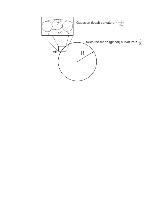
Figure 1: Schematic picture of the mean (global) and Gaussian (local) curvature problem. Twice the mean curvature of the growing sphere of radius $R$ equals $2\over R$ and is a global curvature measure. Upon magnifying the visualisation box (VB) a local picture appears, at a given time instant $t$ and packing conditions $\eta$ (see caption to Figure 2), for which the Gaussian curvature of the building block viz the spherical molecule of radius $r_{mi}$ reads $1\over r_{mi}^{2}$. The overall curvature contribution to the equilibrium BC of Gibbs–Thomson type, Eq. (18), reads $\delta_{T}^{2}\over{r_{mi}R}$, $\delta_{T}$ - Tolman parameter [29], and leads to a modified BC, Eq. (18), of importance for crystal composed of finite-size (or non-point like) building blocks.

As the first essential modification (equilibrium type) of the curvature contribution to the BC we propose to include the Gaussian curvature. Schematic picture of the mean (global) and Gaussian (local) curvature problem is presented in Figure 1. This correction can be important, because of large linear dimension of the growth units in comparison with linear dimension of the other solution components, so the local curvature can play important role, especially when we deal with macromolecular islands built up of a few units. Now the BC takes the form

$$c_{s}=c_{0}(1+2\Gamma{1\over R}+{\delta_{T}^{2}\over r_{mi}}{1\over R})=c_{0}(1+2\tilde{\Gamma}\frac{1}{R}),$$ (24)

where

$$\tilde{\Gamma}=\Gamma+\frac{\delta_{T}^{2}}{2r_{mi}}$$ (25)

and $1/(r_{mi}R)$ is a Gaussian curvature, $r_{mi}$ is the radius of the crystal building unit (for lysozyme protein $r_{mi}\approx 1.5nm$) and $\delta_{T}$ is a Tolman length. $\delta_{T}$ is defined as the difference between the radius of the surface of tension and the radius of the equimolar dividing surface (for lysozyme protein $\delta_{T}\approx 3.5nm$) and depends on the packing coefficient of the crystal. The Tolman length can be related to the superficial density at the surface of tension [29]. Note that by postulating $c_{s}$ in the form of Eq. (24), with $\delta_{T}$ involved, we somehow induce, for a given time instant $t$, elastic effects at the crystal boundary. This is because $\delta_{T}$ is also a measure of rigidity for bending of a curved piece of the crystal boundary, a physical fact well known to those studying biomembrane formation [30]. Thus, we may, also by means of having $\delta_{T}$ involved in the BC, arrive at elastic contribution to the crystal growth [1]: This situation resembles a well-known fact that an improperly placed boundary molecule, or some impurity, exerts an additional strain-stress field in its very vicinity [31].
The solution of Eq. (17) with BC prescribed by Eq. (24), with (25) is of the same type as the one given by Eq. (20) but now

$$R_{c}=\tilde{R_{c}}=2\sigma_{0}\tilde{\Gamma}$$ (26)

has to be inserted, cf. Eq. (23).

The dependence of $R(t)$ is presented in Figure 2. The lower-right inset to Figure 2 shows differences in behavior of the surface concentration with and without Gaussian curvature correction to the surface concentration, while the upper-left inset points to early-stage differences in tempo of crystal formation expressed in terms of $R$ vs $t$ dependence. These differences stand also over longer time period but they cannot be seen as separated curves for time interval ($1.5$ hour) chosen to fit our model to experimental data [32]. We can see that Gaussian curvature influences (speeds up) the growth rate just by increasing the local surface concentration, especially for the early stage of the growth process when $R/r_{mi}$ is relatively small.

Our results adjust well to the experiment. Chow et al. [32] observed constant growth rate of the lysozyme spherulites, what is characteristic when the growth is controlled by surface kinetics rather than by volume diffusion. In the experiment the crystal density is 25 times bigger than lysozyme concentration in the solution. In our calculation supersaturation is equal 500. This discrepancy implies that the narrow interfacial region (double layer) designed for our model is definitely a protein-poor region.

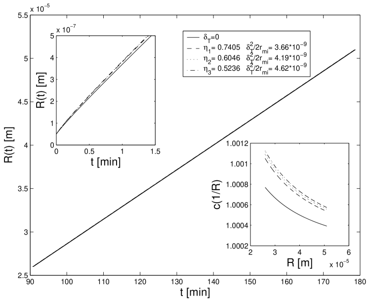
Figure 2: The time dependence of the crystal radius $R(t)$ for original (18) and modified (24) BCs of Gibbs-Thomson (and Tolman) types taken for three different crystal structures (cubic close packing $\eta_{1}$, hexagonal lattice $\eta_{2}$ and cubic lattice $\eta_{3}$). The lower-right inset shows differences in behavior of the surface concentration with and without Gaussian curvature (finite-size or Tolman type) correction to the surface concentration, while the upper-left inset points to early-stage differences in tempo of crystal formation. These differences stand also over longer time period but they cannot be seen as separated curves for time interval chosen to fit our model to experimental data ($C=500$ [arbitrary units], $c_{0}=1$ [arbitrary units], $\Gamma=1\cdot 10^{-8}m$, $R_{c}=4\cdot 10^{-11}m$, $R_{0}=5\cdot 10^{-8}m$, $v_{mi}=2.3\cdot 10^{-6}m/s$).

In the second case we propose ”Goldenfeld-type” correction [27]. Now we assume that the surface is away from local equilibrium and deviation from this state is proportional to the growth velocity of the interface

$$c_{s}=c_{0}(1+2\tilde{\Gamma}\frac{1}{R}-\beta_{G}\frac{dR}{dt}),$$ (27)

where $\beta_{G}$ is a positive kinetic coefficient. Solving Eq. (17) with nonequilibrium boundary condition, Eq. (27), one gets for long times the linear solution of exactly the same type than that given by (21) which can reflect the asymptotic temporal behavior of spherulites. It can be shown that when $\beta_{G}$ increases the growth becomes slower. At early stage of the growth process the influence of $\beta_{G}$ on $R(t)$ is strongly nonlinear. For long times, the growth is linear in time and $\beta_{G}$ influences only the growth rate (slope of the curve, cf. Figure 2) [2].

Looking at the Eq. (17) we can see that the growth process depends not only on the supersaturation of the solution. It turns out to be very important that the macroion velocity, which depends on the electrostatic interactions of the macroion with the solution (we have to mention that the solution is an electrolyte), also depends on the viscosity of the solution, and moreover, on the size of the growth units. It is sometimes possible that the growth unit will be made of few macromolecules, so that in the viscoelastic complex environment that we actually describe, the aggregates (made up of $2-5$ macromolecules) will have different velocities, especially when compared with that of the single macroion because the diffusion coefficient can now be aggregate-size dependent [33]. This experimentally justified observation [34] has its profound impact on the so-called intrinsic properties of the viscoelastic solution [16], making them time-sensitive, thus imposing an intrinsic time scale, presumably powerly ”correlated” with the observation time scale [35]. It will be demonstrated in the subsequent section.

4 Sphere growth controlled by convective fluctuations: the role of time-dependent viscosity and finite-size effects

In accordance with the considerations of the previous section, here we will complement the deterministic description of the kinetics of crystal growth by incorporating thermal fluctuations of the bath through fluctuations of the velocity of the incoming macroions (or growth units) [36], and relating them with the finite size of the particles at the locally highly concentrated regime. In this regime, the viscoelastic properties of the solution become important and must also be incorporated into a consistent description.

To perform this description, we will adopt an effective medium theory [37] in which the diffusion of a ”test” macroion through a saturated solution can be analyzed in terms of the single-particle distribution function $f(\vec{r},\vec{u},t)$, depending on the position $\vec{r}$ and instantaneous velocity $\vec{u}$ of the macroion. In accordance with mesoscopic nonequilibrium thermodynamics formalism, in this case the entropy per unit volume, $s(t)$, can be expressed in terms of the Gibbs entropy postulate [37, 38]

$$s(t)=s_{le}-k_{B}\int f\ln\frac{z}{z_{le}}d\vec{u},$$ (28)

where $s_{le}$ is the entropy at local equilibrium, cf. Eq. (1), and we have introduced the fugacity $z=\alpha\,f(\vec{r},\vec{u},t)$, with $\alpha$ the activity coefficient characterizing the interactions of the macroion. $z_{le}$ is the fugacity at local equilibrium. The activity coefficient $\alpha$ will contain two contributions since the test macroion interacts with both, the solution of macroions $\alpha_{s}$ (mostly, in the vicinity of the crystal boundary) and with the crystal $\alpha_{c}$, see Figure 3. The activity of the solution can be expressed as $\alpha_{s}=e^{c^{-1}p/k_{B}T}$, with $c^{-1}p$ the compressibility factor in which $p$ is the excess of osmotic pressure [37] and the concentration field is defined by $c(\vec{r},t)=\int f(\vec{r},\vec{u},t)d\vec{u}$. The explicit expression of $c^{-1}p$ can be obtained in the context of different theories on electrolyte solutions [39]. The crystal activity $\alpha_{c}$ can, in general, contain effects related with entropic, energetic or geometrical constrains, as indicated in section 2, [1].

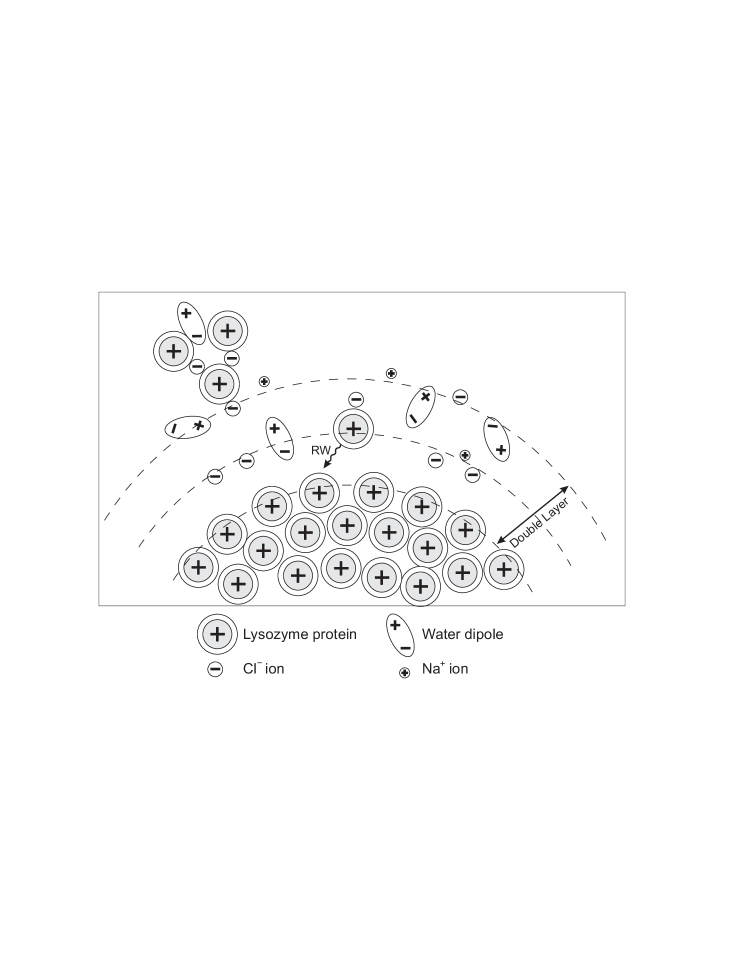
Figure 3: Naive picture of the vicinity of the crystal surface. Building unit (positively charged lysozyme protein), which is surrounded by neutral (water dipoles) and oppositely charged particle (counterions), performs random walk (RW) with a constant velocity in an electrostatic double layer. We can see that the crystal surface is not smooth and the local (Gaussian) curvatures are shown (see caption to Figure 1). In the left top corner a triplet has already been formed.

Following the procedure of MNET already outlined, one may show that the Fokker-Planck equation describing the evolution of $f(\vec{r},\vec{u},t)$ is [37, 40]

$$\frac{\partial f}{\partial t}+\nabla\cdot\left(\vec{u}f\right)-k_{B}T\nabla\left[\ln\alpha_{c}+\ln\alpha_{s}\right]\cdot\frac{\partial f}{\partial\vec{u}}=\frac{\partial}{\partial\vec{u}}\cdot\beta(t)\left[\vec{u}f+\frac{k_{B}T}{m}\frac{\partial f}{\partial\vec{u}}\right],$$ (29)

where the third term on the left-hand side of the equation contains the forces acting on the macroion. The right-hand side of this equation contains the contributions of Brownian motion of the macroion in which the time-dependent friction coefficient $\beta(t)$ introduces memory effects [41, 42]. As mentioned in the previous section, these effects are related to the viscoelastic properties of the solution (time-dependent viscosity), and modify the intrinsic time scale of the particle dynamics.

Several models for the friction have been used in the literature of model crystal growth [36]. However, since we are interested in analyzing the effects of the finite size and inertia of the macroions, then we must take into account that in this case a general expression for the friction coefficient is [40, 37]: $\beta^{-1}(t)\propto{\cal L}^{-1}\left[1+\left(\tau_{D}\omega\right)^{\gamma_{c}}\right]^{-1}$, with the symbol ${\cal L}^{-1}$ denoting the inverse Laplace transform, $\omega$ the frequency and $\tau_{D}=\frac{r^{2}_{mi}}{D_{0}}$ a characteristic diffusion time, with $D_{0}=\frac{k_{B}T}{6\pi\eta_{id}r_{mi}}$ the diffusion coefficient of the macroion at infinite dilution, $r_{mi}$ is the macroion radius and $\eta_{id}$ the viscosity of the solvent at infinite dilution. In this relation, the exponent $\gamma_{c}$ may in general be a function of the macroion concentration at the bulk [37]. In order to make an analytical progress, for simplicity one may use the expression of $\beta(t)$ obtained in the context of the generalized Faxén theorem [40, 43]

$$\beta^{-1}(t)=\beta^{-1}_{0}\left[\sqrt{\frac{\tau_{D}}{t}}-exp\Bigg{(}{\frac{t}{\tau_{D}}}\Bigg{)}Erfc\left(\sqrt{\frac{t}{\tau_{D}}}\right)\right],$$ (30)

where $\beta_{0}=6\pi\eta_{id}r_{mi}$ is the Stokes friction coefficient. Notice that Eq. (30) is the inverse Laplace transform of $\beta^{-1}(\omega)=\beta^{-1}_{0}\left[1+(\tau_{D}\omega)^{1\over 2}\right]^{-1}$, and that at times $t<<\tau_{D}$, it reduces to $\beta^{-1}_{0}\sqrt{\frac{\tau_{D}}{t}}$.

To obtain the velocity $\vec{v}(t)$ of the macroions entering into the growth rule (17) in which, however, the macroion velocity has been assumed constant, see legend to Figure 2, one may use Eq. (29) to obtain the hierarchy of evolution equations for the moments of $f$, and from it construct the equation [37]

$$\frac{\partial c}{\partial t}=-k_{B}T\nabla\cdot\left[\beta^{-1}c\nabla\ln\alpha_{c}\right]+\nabla\cdot\left[D_{c}\nabla c\right].$$ (31)

which describes the evolution of the macroion in the diffusion regime. Here, we have defined the collective diffusion coefficient $D_{c}\equiv k_{B}T\beta^{-1}\left(1+\frac{\partial\ln\alpha_{s}}{\partial\ln c}\right)$. Particular expressions for this coefficient can be modelled within the scope of, for example, Kirwood theory of solutions. In a mean field approximation, the pressure $p$ can be approximated by an expansion of the form $pk_{B}T\left[c-B(T)c^{2}\right]$, where $B(T)$ is a virial-type coefficient incorporating the specificities of the pairwise interactions among macroions. In general, $B(T)$ may depend on the radial distribution function, and then on spatial correlations. Substituting this expansion into $\alpha_{s}=e^{c^{-1}p/k_{B}T}$, taking the logarithm and the corresponding derivative of the definition of $D_{c}$, one obtains the time-dependent diffusion coefficient $D_{c}=k_{B}T\left(1-B(T)\right)\beta^{-1}(t)$.It is interesting to notice that $T\left(1-B(T)\right)$, resembling an ”effective” temperature [37], implies that macroion diffusion has a nonlinear dependence on $T$, which could be relevant in the crystal structure, as was already mentioned. From Eq. (31), it follows that in the diffusion regime the velocity of the macroions will satisfy a Langevin equation of the form

$$\frac{dr(t)}{dt}=v(t)=\beta^{-1}(t)\left[F_{d}(t)+F^{R}(t)\right],$$ (32)

where for simplicity we have considered the unidimensional case and $F^{R}(t)$ constitutes a random force due to thermal fluctuations. Moreover, we have defined the deterministic force $F_{d}(t)=\int\left[k_{B}T\frac{d\ln\alpha_{c}}{dr}\right]c(r,t)dr$, due to the interaction of the macroion with the crystal. Notice that the fluctuating part of the velocity satisfies the usual conditions of zero mean and $\langle v(t)v(t_{1})\rangle=\beta^{-1}(t-t_{1})$ [41].

In a first approximation, one may assume that in the vicinity (double layer) of the crystal surface, the electrostatic force (attracting macroions) is constant, $F_{d}=F_{0}$, [12]. This assumption implies that $\alpha_{c}$ depends upon the minimum reversible work necessary to move the macroion a certain distance $\Delta r$, $\alpha_{c}=e^{F_{0}\Delta r/k_{B}T}$, see Eq. (3). On taking into account the above assumptions, near to the crystal, the growth rule (17) can be written in the approximated form

$$\frac{dR(t)}{dt}=\sigma_{R}\beta^{-1}_{0}\sqrt{\frac{\tau_{D}}{t}}\left[F_{0}+F^{R}(t)\right]$$ (33)

where $\sigma_{R}=\frac{c_{s}}{C-c_{s}}$. In the present approximation, $\sigma_{R}$ can, for instance, be expressed in the form

$$\sigma_{R}=\sigma_{0}\frac{1+{2\tilde{\Gamma}\over R}}{1-{2\tilde{R}_{c}\over R}},$$ (34)

after using Eqs. (24), (25) and (26). Note that for $t>>1$ $\sigma_{R}\to\sigma_{0}$ holds. Moreover, notice that for $c_{s}$ we have to take here, depending on what we wish to model, either $c_{s}$ from (24) (equilibrium BC: non-Kossel crystals) or the one from (27) (nonequilibrium BC: biopolymeric spherulites). Especially, the latter seems to be a challenge for extensive numerical modeling, which is, however, left for a future task. In both cases mentioned, however, the FSE account is thoroughly manifested, cf. Figs 1-4.

Now, in order to show the relation existing between the present approach with that of Sec. 2, for simplicity we will consider the case in which the deterministic part $F_{0}$ can be neglected. As a consequence, Eq. (33) becomes a stochastic equation with multiplicative noise which is equivalent to the Fokker-Planck equation [36]

$$\frac{\partial P(R,t)}{\partial t}=\frac{\partial}{\partial R}\left[D(R,t)\frac{\partial P(R,t)}{\partial R}+\frac{D(R,t)}{k_{B}T}\frac{\partial\Phi}{\partial R}P(R,t)\right],$$ (35)

where $P(R,t)$ is the probability density in the $R$-space with $R$ standing for the radius of the spherical crystal. Moreover, we have defined the potential $\Phi\equiv\ln\sigma_{R}$ and the diffusion coefficient

$$D(R,t)\equiv D_{R}(t)\sigma_{R}^{2},$$ (36)

where

$$D_{R}(t)=D_{0}\sqrt{\frac{t}{\tau_{D}}}$$ (37)

is the time-dependent diffusion coefficient of the incoming macroions related with $\beta^{-1}$ through [36]

$$D_{R}(t)=k_{B}T\int^{t}_{0}\beta^{-1}(t_{1})dt_{1}.$$ (38)

Figure 4, shows the time-dependent part of the reduced diffusion coefficient as a function of the reduced time. The solid line represents the integral of Eq. (30), whereas the short-dashed line is represented by Eq. (37), see Eq. (36). The long-dashed line represents a $t^{\frac{1}{4}}$ behavior for comparison. From the solid line it follows that at short times the crystal grows with a superdiffusive behavior whereas at larger times, $D_{R}$ tends to a constant value, implying that the crystal radius tends to a maximum value, i.e. to a final equilibrium state. It coincides well with both the deterministic view of the process, and above all, with its experimental realizations [15, 31]. It is interesting to realize that formally both the growth speed and the constrained motion of a ’representative’ macroion, feeding the crystal go in a superdiffusive way. Thus, it seems that both sub-processes manifest a kind of synchronous temporal behavior.

Finally, notice that from equation (35) it follows that the deterministic part of the current is

$$J(R,t)=-\frac{D(R,t)}{k_{B}T}\frac{1}{\sigma_{R}}\frac{\partial\sigma_{R}}{\partial R}.$$ (39)

Comparing this expression with Eq. (12), one may conclude that $\sigma_{R}$ plays the role of a fugacity in $R$-space whereas $\Phi$ the role of a chemical potential containing geometric restrictions due to the boundary conditions, as discussed in the previous section [18].

Figure 4: Reduced diffusion coefficient $\frac{D_{R}}{D_{0}}$ as a function of the reduced time $\frac{t}{\tau_{D}}$, for $D_{0}\simeq 10^{-6}cm^{2}s^{-1}$ and $\tau_{D}\simeq 10^{-8}s$. The solid line represents the integral of Eq. (30), whereas the short-dashed line is represented by Eq. (37). In the deterministic case, the integration of Eq. (33) can be compared with that of Eq. (20) with the parameters $\tilde{\Gamma}$ and $\tilde{R}_{c}$, from which follows that at sufficiently large times the left-hand side behaves as $R$, whereas the right hand side will be proportional to Eq. (38). Since the solid line tends to a constant asymptotic value, then from the figure it follows that for sufficiently long times, the radius of the crystal tends to a maximum value. In contrast, $\beta^{-1}_{0}\sqrt{\frac{\tau_{D}}{t}}$ implies a ”pure” superdiffusive growth. The long-dashed line, corresponding to a $t^{\frac{1}{4}}$ behavior, has been included for comparison. It can be obtained form $\beta^{-1}(t)\propto{\cal L}^{-1}\left[1+\left(\tau_{D}\omega\right)^{\gamma_{c}}\right]^{-1}$, when the exponent $\gamma_{c}=1/4$.

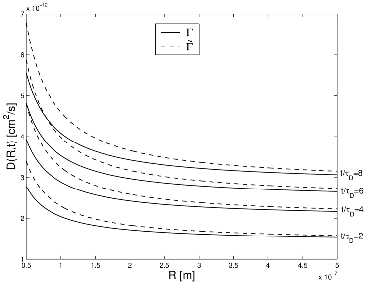
Figure 5: Mean course of the overall diffusion-type behavior of the non-Kossel (model) crystal growth. The curvature effect and FSE are largely pronounced for $\gamma_{c}={1\over 2}$ and some consecutive time steps $t$. The same type of temporal behavior has been proposed in [36] for algebraic correlations with exponent $\gamma_{c}={1\over 2}$. Solid lines are plotted on the basis of Eq. (36), whereas the dashed lines on its equivalent with $\tilde{R_{c}}=R_{c}$ and $\tilde{\Gamma}=\Gamma$ (for details see caption to Figure 4).

5 Summary and conclusions

In this paper, we have proposed an integrated static-dynamic picture of model (spheroidal) crystal growth in a complex milieu, preferentially of electrolytic type. The complex milieu we have in mind here could, in general, be a two-component system, containing some impurities and/or (charged) additives. The spectrum of examples can range from metallic polycrystals ($L-M-H$ model, sec. 2.1 and 2.2) via superconductors ($U-C-J$, sec. 2.3) until the soft-condensed matter objects that are: non-Kossel crystals and (bio)polymeric spherulites. In fact, the latter suits best our type of modeling since it really manifests the FSE property due to pronounced sizes of the macromolecules constituting the (dis)ordered macromolecular cluster. The goal of readily incorporating the FSE property into the growth rules governing spheroidal crystal formation has been successfully achieved at both static as well as dynamic level of description - therefore our integrated model is called static-and-dynamic. At the static level of description the goal has been achieved by proposing a modification of the well-known Gibbs-Thomson (equilibrium) formula or by additionally including its nonequilibrium modification that we attributed to Goldenfeld, who likely did it for the first time almost twenty years ago but for a diffusive field feeding the growing object [27]. In this study, however, we have concentrated on the equilibrium BC with the Tolman-type correction proposed, emphasizing a pivotal role of the Gaussian curvature in the realistic view of the process that we have offered. Therefore, the nonequlibrium type BC is dealt with in a rather sketchy or qualitative way, but nevertheless, such a possible modification is worth mentioning, at least for some interesting future task. Some undoubtful integrity of the picture, or its quite comprehensive character, at which we have finally arrived, can by no means be accomplished when no complementary stochastic part had a chance to appear. This is, in our opinion, the most worth-emphasizing part of the description, very responsible for unveiling its dynamic aspects. It could also be worth-presenting when forseeing a necessity to go beyond some analytic modeling [37, 22, 18, 36], and to propose thoroughly computer simulations, carried out in a complementary way [6, 24, 26]. Thus, the integrated static-dynamic picture of the process is offered in sec. 4. It tells us that: (1) the role of curvature(s) is important; (2) the role of FSE is equally important, and anticipates the approach to be quite realistic; (3) the role of velocity fluctuations in time appears to be crucial in setting up properly the picture: a basic result of sec. 4 points to the constrained motion of the macroion to be superdiffusive, with the exponent $1/2$ for an unidimensional approximation offered therein. Thus, and in particular, a specific goal to propose a firm mathematical form for algebraic correlations, somehow underscored in another study [36] has been achieved too. The account of correlations in space is not explicitely taken into account in this study. Implicitely, however, it is involved in it by proposing Eq. (31) with the collective measure, $D_{c}$, from which further a Langevin-type as well as Fokker–Planck type descriptions for model crystal growth (within the integrated picture) arise. What above all comes out from the proposed integrated picture, however, is a clear dynamic measure of this integrity, represented by $D(R,t)$ of Eq. (36). It is seen in a picturesque way in Fig. 5 which tells us that the process goes naturally in the way that for its final (mature) growing stages the overall diffusivity of the system, due to the above mentioned physical factors (FSE, curvature(s), fluctuations) slows down, this way likely promoting order against disorder in the complex entropic milieu from which the object emerges. Also, a difference between Gaussian and non-Gaussian curvature effects on the diffusive behavior of the system clearly pronounce in the course of time. Finally, let us underline a remarkable feasibility of the presented type of modeling to serve for fitting to some experimental curves, or to relate the proposed theory to the experiment. An example of such an ability has been offered by Fig. 2, i.e. the case of biopolymeric spherulites, for the kinetic coefficient, ${\beta_{G}}\to 0$, i.e. when the nonequilibrium BC gets finally equilibrated. Other fits can be done for non-Kossel crystals as well [31, 15]. Last but not least, let us juxtapose some features of MNET, because this thermodynamic-kinetic formalism enabled to offer such an integrated view of the process. These are [14, 5, 43, 42]:

• MNET provides a description of kinetic proceses taking place at the mesoscale (and involving mesostructures) in which fluctuations are important.

• The theory provides in general expressions for the rates (nucleation, growth, reaction, etc.) which are in general nonlinear functions of the driving forces. They are derived in very general conditions even when mesostructures are embedded in an inhomogeneous bath.

• The theory provides kinetic equations of the Fokker–Planck type for the evolution of the probability distribution. From them one can derive expressions for the moments of the distribution which are related to physical quantities which can be compared with experiments.

References

- [1] A. Gadomski, J. Siódmiak, Phys. Status Solidi B (2004) - in press.
- [2] A. Gadomski, J. \aLuczka, Inter. J. Quantum Chem. 52, 301 (1994).
- [3] Statistical and Dynamical Aspects of Mesoscopic Systems, Eds.: D. Reguera, G. Platero, L. L. Bonilla, J. M. Rubi, Lecture Notes in Physics, Springer, Berlin Heidelberg 2000.
- [4] I. Santamaría-Holek, PhD Thesis, University of Barcelona, June 2003.
- [5] D. Reguera, J. M. Rubí, L. L. Bonilla, in: V.Capasso (Ed.), Mathematical Modelling for Polymer Processing, Mathematics in Industry Series, Vol. 2, Springer, Berlin 2002, chap. 3.
- [6] R. Cloots, N. Vandewalle, M. Ausloos, Appl. Phys. Lett. 65, 3386 (1994); Appl. Phys. Lett. 67, 1037 (1995).
- [7] A. A. Chernov, J. Mat. Sci.: Materials in Electronics 12, 437 (2001).
- [8] S. R. de Groot, P. Mazur, Non-Equilibrium Thermodynamics, Dover Publications, London 1984.
- [9] D. Thirumalai et al., Curr. Opin. Struc. Biol. 13, 146 (2003).
- [10] P. Reimann, Phys.Rep. 361, 57 (2002).
- [11] K. Bochenek, E. Gudowska–Nowak, Chem. Phys. 373, 532 (2003).
- [12] A. Gadomski, J. Siódmiak, Cryst. Res. Technol. 37, 281 (2002).
- [13] Forces, Growth and Form in Soft Condensed Matter: At the Interface between Physics and Biology Proceedings of the NATO Advanced Study Institute, Geilo, Norway, from 24 March to 3 April 2004, NATO Science Series II: Mathematics, Physics and Chemistry, Vol. 160, Eds.: A. T. Skjeltorp, A. V. Belushkin, 2004.
- [14] J. M. G. Vilar, J. M. Rubí, Proc. Natl. Acad. Sci. USA 98, 11081 (2001).
- [15] P. Vekilov, H. Lin, F. Rosenberger, Phys. Rev. E 55, 3202 (1997).
- [16] A. Plonka, Dispersive Kinetics, Kluwer, Dordrecht 2001.
- [17] J. Drenth, Principles of Protein X-ray Crystallography, Springer-Verlag, New York 1999.
- [18] J. M. Rubí, A. Gadomski, Physica A 326, 333 (2003).
- [19] N. G. van Kampen, Stochastic Processes in Physics and Chemistry, North-Holland, Amsterdam 1987.
- [20] L. D. Landau, E. M. Lifshitz, L. P. Pitaevskii, Physical kinetics (Course of Theoretical Physics) Vol. 10, Pergamon Press, Oxford 1981.
- [21] V. A. Shchukin, D. Bimberg, T. P. Munt, D. E. Jesson, Phys. Rev. Lett. 90, 076102 (2003); D. E. Jesson, T. P. Munt, V. A. Shchukin, D. Bimberg, Phys. Rev. Lett. 92, 115503 (2004).
- [22] A. Gadomski, J. M. Rubí, Chem. Phys. 293, 169 (2003).
- [23] P. A. Mulheran, Acta Metall. Mater. 40, 1827 (1992); N. P. Louat, Acta Metall. 22, 721 (1974).
- [24] M. Ausloos, N. Vandewalle, R. Cloots, Europhys. Lett. 24, 629 (1993); M. Ausloos, N. Vandewalle, Acta Phys. Pol. B 27, 737 (1996).
- [25] D. R. Uhlmann, B. Chalmer, K. A. Jackson, J. Appl. Phys. 35, 2986 (1964).
- [26] N. Vandewalle, M. Ausloos, R. Cloots, Phil. Mag. A 72, 727 (1995).
- [27] N. Goldenfeld, J. Cryst. Growth 84, 601 (1987).
- [28] K. Huang, Statistical Mechanics, John Wiley & Sons, New York 1963, chap. 2.
- [29] R. C. Tolman, J. Chem. Phys. 17, 333 (1949).
- [30] E. M. Blockhuis, J. Groenwold, D. Bedeaux, Molec. Phys. 96, 397 (1999).
- [31] P. Vekilov, J. I. D. Alexander, Chem. Rev. 100, 2061 (2000).
- [32] P. S. Chow, X. Y. Liu, J. Zhang, R. B. H. Tan, Appl. Phys. Lett. 81, 1975 (2002).
- [33] L. de Arcangelis, E. del Gado, A. Coniglio, in International Workshop and Collection of Articles Honoring Prof. Antonio Coniglio, Eds. R. Family et al. World Scientific Publishing 2002, p. 9.
- [34] J.E. Martin, A. Douglas, J.P. Wilcoxon, Phys. Rev. Lett. 61, 2620 (1988).
- [35] B. B. Mandelbrot Fractals: Form, Chance, and Dimension, Freeman, San Francisco 1982, chap. 12.
- [36] J. \aLuczka, M. Niemiec, R. Rudnicki, Phys. Rev. E 65, 051401 (2002).
- [37] J. M. Rubí, I. Santamaría-Holek, A. Pérez-Madrid , J. Phys. Cond. Matt. 16, 2047 (2004).
- [38] A. Pérez-Madrid, J. M. Rubí, P. Mazur, Physica A 212, 231 (1994).
- [39] T. R. Hill, An introduction to statistical thermodynamics, Dover, New York 1986.
- [40] I. Santamaría-Holek, J. M. Rubí, A. Pérez-Madrid, cond-mat/0409362.
- [41] S. A. Adelman, J. Chem. Phys. 64, 124 (1976).
- [42] I. Santamaría-Holek and J. M. Rubí, Physica A 326, 384 (2003).
- [43] R. Morgado, F. A. Oliveira, Phys. Rev. Lett. 89, 100601 (2002).