Critical indices of random planar electrical networks

Abstract

We propose a new method to estimate the critical index $t$ for strength of networks of random fused conductors. It relies on a recently introduced expression for their yield strength. We confirm the results using finite size scaling. To pursue this commitment, we systematically study different damage modalities of conducting networks inducing variations on the behavior of their nonlinear strength reduction.

I Introduction

Random resistor networks are used to model a variety of physical phenomena ranging from the properties of inhomogeneous media S. Redner and H. E. Stanley (1979); M. Sahimi and J. D. Goddard (1985); J. W. Chung, A. Ross, J. Th. De Hosson and E. van der Giessen (1996); P. Ray and B. K. Chakrabarti (1988); Y. Kantor and I. Webman (1984), to metal insulator transitions V. K. S. Shante and S. Kirkpatric (1971), dielectric breakdown H. Takayasu (1985); J. C. Dyre and Th. B. Schoder (2000); A. Hansen, E. L. Hinrichsen and S. Roux (1991a, b), the role of percolation in weak and strong disorder C. Tsallis and S. Redner (1983); Zhenuhua Wu, Eduardo López, Sergey V. Buldyrev, Lídia A. Braunstein, Shlomo Havlin, H. Eugene Stanley (2005); Guanlian Li, Lídia A. Braunstein, Sergey V. Buldyrev, Shlomo Havlin, H. Eugene Stanley (2007), and the strength of trabecular bone Y. C. Fung (1993); K. G. Faulkner (2000); G. H. Gunaratne, C. S. Rajapakse, K. E. Bassler, K. K. Mohanty and S. J. Wimalawansa (2002). Essentially, this study intends to develop a method to establish a relationship between the mean strength of bone and its mass. In fact, large bones consist of an outer compact shaft and an inner porous region, i.e., a trabecular architecture whose structure is reminiscent of a complex system of disordered networks. The bone strength depends on many factors, i.e., architectural characteristic (level of connectivity), perforation, thinning, anisotropy, as well as subarchitectural properties of bone like the mineral content, the density of the diffuse damage. A significant mechanism for loss of trabecular mass is through the removal of individual struts, due to traumatic events. Mechanical studies on ex vivo bone samples have shown that trabecular networks from patients with a broad range of age fracture at a fixed level of strain E. F. Morgan and T. M. Keaveny (2001), even though the corresponding fracture stresses exhibit large variations. These observations have motivated the induced fracture criteria utilised in our models.

We consider the lattice network of conducting disordered elements to study the essential non-linear and irreversible properties of the electrical breakdown strength. Subjecting the system under extreme perturbation, its electrical properties tend to get destabilised and so that failure breakdown occurrences. In fact, these instabilities in the system often nucleates around disorder, which plays a major role in the breakdown properties of the system. The growth of these nucleating centers, in turn, depends on various statistical properties of the disorder, namely the scaling properties of percolation structures, its fractal dimensions, etc. By increasing the percentage number of the network nonconducting elements, its conductivity decreases, so also does the breaking strength of the material, the fuse current of the network decreases on the average with the increased concentration of random impurities.

We are considering here the problem associated with failures in disordered system under the influence of an electrical field. In spite of this framework is shown simpler than the one related to mechanical failure of fractures, however all these cases of failures present some common features. In particular, certain features near breakdown agree with those of resistor networks close to the percolation threshold B. K. Chakrabarti and L. G. Benguigui (1997); P. M. Duxbury, P. D. Beale and P. L. Leath (1986a, b); H. J. Herrmann, A. Hansen and S. Roux (1989). This article presents a systematic new method to estimate critical indices by quantifying the reduction of current in fused resistor networks.

The model and the expression which relate the strength reduction to the statistical properties of disorder network system is set up in section II. We focus on fractured conducting networks to examine many possibilities for. Initially, it is supposed that disorder just arises from random percolation. Both cases are considered, the isotropic and the anisotropic conducting networks. Next, it is also considered that the failure current of the conducting network are not the same, but it is being uniformly distributed in a range, in addition to random uniform percolation. This issues are presented and quantified in Section III. Finally, Section IV is devoted to conclusions.

II The Model

We take square networks consisting of fused conductors that fail when the potential difference across them reaches a pre-set value;  i.e., the breakdown current of an element is proportional to its conductance. Typically, failure of an element increases currents on neighboring conductors, enhancing the likelihood of their failure J. W. Esam (1980); D. Stauffer and A. Aharony (1992). We study the yield point at which the external current initiates the first failure. The peak currents on a network show similar behavior P. M. Duxbury, R. A. Guyer and J. Machta (1995).

Consider first, a complete square network of size $M\times\,M$, with the top and the bottom edges at potentials $V_{0}$ and $0$ respectively. Assume that each electrical element in the network fails when the potential difference across it reaches a value $V_{b}$. We can calculate the current $I(0)$ flowing through the network using Kirchhoff’s laws. As $V_{0}$ increases, currents through the conductors, as well as $I(0)$, will increase until the yield point $I(0)=I_{yield}(0)$, where the first failure occurs.

Next consider a network, where we have attempted to remove elements with a probability $p$. Denote the yield current of such a network by $I_{yield}(p)$. Typically, $I_{yield}(p)$ decreases with increasing $p$, and vanishes as $(p_{0}-p)^{t}$ when $p$ approaches the percolation threshold $p_{0}\,$(=0.5 for isotropic square networks). $t$ is the critical index, with reported values between $1.1$ and $1.43$ under different scenarios of damage and symmetries of the network C. J. Lobb and D. J. Frank (1979); S. Kirkpatrick (1973, 1978); Y. Gefen, A. Aharony, B. B. Mandelbrot and S. Kirkpatrick (1981); L. Benguigui (1986); B. I. Halperin, S. Feng and P. N. Sen (1985); D. J. Frank and C. J. Lobb (1988); B. I. Halperin (1989); M. Sahimi (1994).

There have been several proposals related to the form of the reduction of strength of a network due to a random removal of elementP. M. Duxbury, P. D. Beale and P. L. Leath (1986a); B. K. Chakrabarti and L. G. Benguigui (1997). Here we test a recently proposed expression for $I_{yield}(p)$ J. S. Espinoza Ortiz, Chamith S. Rajapakse and Gemunu H. Gunaratne (2002):

$$\tau(p)\equiv\frac{I_{yield}(p)}{I_{yield}(0)}=\frac{1}{1\,+\,a_{1}\,z\,^{t/2}\,+\,a_{2}\,z\,^{t}}\,,$$ (1)

where $z=\log(N)/\log(\frac{p_{0}}{p})$. Here, $N(=M^{2})$ is the number of nodes in the original network, $p_{0}$ is the bond percolation threshold for the class of network considered, and $a_{1}$ and $a_{2}$ are constants that depend on model parameters as discussed below. Observe that, as $p\rightarrow p_{0}$, the yield strength, $\tau(p)\rightarrow(p_{0}-p)^{t}$. We conjecture that Equation (1) is valid throughout the range $p\in[0,p_{0})$, we use this conjecture to estimate $\,p_{0}$ and the critical index $t\,$ ; then validate it using finite size scaling method.

We compute the yield current for a given network as follows: given the conductance $\sigma_{i}$ of all electrical elements in the network and the potential $V_{o}$ of the top layer of nodes, we use Kirchhoff’s laws to determine the currents $i_{k}$ through each element and the potential differences $v_{k}$ across them. We denote the largest of the latter by $V_{max}$. The current $I(p)$ passing through the network is the average of all currents through electrical elements belonging to a fixed horizontal layer. The yield current is $I_{yield}(p)=I(p)\times\,V_{b}/V_{max}$.

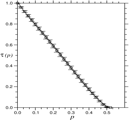
Figure 1: Strength reduction in a $160^{2}$ network due to a random isotropic removal of a fraction $\,p\,$ of conductances, averaged over one thousand trials. Numerical results are shown by boxes along with the statistical error, while those obtained by fitting to expression (1) are shown as a continuous line.

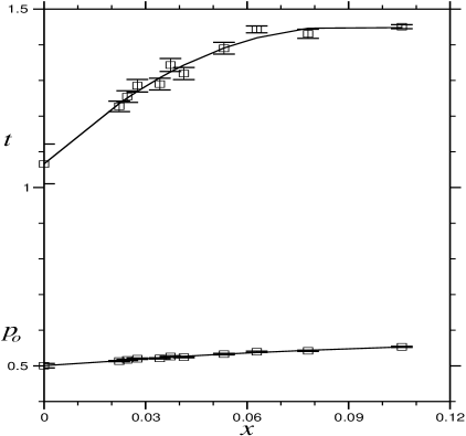
Figure 2: Variation of parameters $t$ and $p_{0}$ versus the inverse correlation length $(\,x=M^{-0.75}\,)$, for networks of size  $M=20$ to $M=160$. All elements in the initial networks have conductance of 1 unit. Note that, both critical values for $t\,(=1.066\pm\,0.056)$ and $p_{0}\,(=0.500\pm\,0.006)$ are getting in the limit when $x\rightarrow\,0$.

III Results and Discussions

Our computations used networks with sizes $M=20,\,30,\,40,\,50,\,70,\,80,\,90,\,120,\,140$ and $160$, and sample sizes of $10,000$ for $M=20,\,30,\,40,\,50$, sample size of $2,500$ for $M=70,\,80,\,90$ and finally sample size of $1,000$ for $M=120,\,140,\,160$. Figure 1 shows the behavior of $\tau(p)$ for the $160\times\,160$ networks, where the error bars show standard errors. Although fluctuations $\delta\tau$ in $\tau(p)$ decrease as $p\rightarrow p_{0}$, the relative fluctuations ($\delta\tau/\tau$) increase. The solid line shown in Figure 1 represents the best fit to Equation (1) with parameters $a_{1},\,a_{2},\,p_{0}$ and $t$ in a $160^{2}$ conducting network. To determine their values, $a_{1}=-0.1043\pm\,0.005,\,a_{2}=0.061\pm\,0.003,\,p_{0}=0.513\pm\,0.002$ and $t=1.228\pm\,0.015$, we used the Lavenberg-Marquadt method to implement the nonlinear fit W. H. Press, S. A. Teukolsky, W. T. Vetterling and B. P. Flannery (1988). We must fit $t$ and $p_{0}$ because they depend on the size of the network.

Next, we determine how $p_{0}$ and $t$ change with the network size. We express the parameters as a function of $x=M^{-1/\nu}$ where $\nu$ ($=4/3$ for 2D square networks) is the universal correlation length exponent M. P. M. den Nijs (1979); Yu A. Dzenis and S. P. Joshi (1994);  i.e, $x$ is the inverse of the mean size of the largest domain in a network of size $M\times\,M$. Figure 2 shows the values of $t(x)$ and $p_{0}(x)$, along with the error estimates.

We estimate the value of $t(0)$ corresponding to an infinite network by first approximating $t(x)$ by a rational function $f(x)/g(x)$ (where $f(x)$ and $g(x)$ are polynomials of order $3$ and $2$ respectively) and extrapolating to $x=0$. The values of the extrapolation corresponding to Figure 2 are $p_{0}(0)=0.500\pm\,0.006,\,t(0)=1.066\pm\,0.056,\,a_{1}(0)=-0.106\pm\,0.015\,$ and $\,a_{2}(0)=0.060\pm\,0.004$. The error estimate includes both errors at each $M$ and those due to the extrapolation W. H. Press, S. A. Teukolsky, W. T. Vetterling and B. P. Flannery (1988).

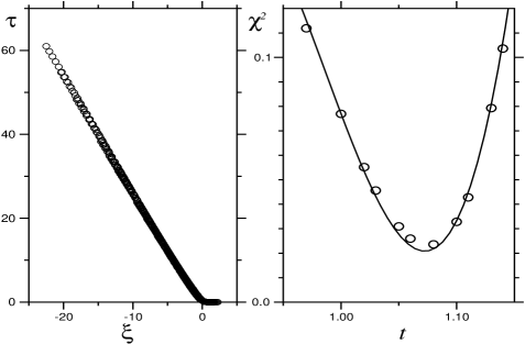
Figure 3: The left side of the figure shows the scaling function ($\tau$) behavior as a function of the network correlation length ($\xi$), and its $\chi^{2}$ error as a function of $t$ for fixed unit conductances in the network (right side). The minimum of $\chi^{2}$ is $t$, gives the critical exponent.

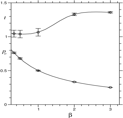
Figure 4: Values of $t(\beta)$ and $p_{0}(\beta)$ with $\beta$, for anisotropic removal of conductance. Elements in the vertical and horizontal directions are removed with probabilities $p$ and $\beta\,p$.

We now validate our results using finite size scaling to independently estimate $t(0)$. According to the finite size scaling ansatz, for the correct $t(0)$, the relationship between the rescaled variables $\overline{\tau}=M^{t(0)/\nu}\times\tau$ and $\zeta=M^{-1/\nu}(p_{0}-p)$ is independent of the system size $M$ M. E. J. Newman and G. T. Barkema (2001). Although the finite size scaling ansatz need hold only for $p\rightarrow\,p_{0}$ (and $0<M^{-1/\nu}<1$), we find that the data collapses to a scaling function $\overline{\tau}(\zeta)$ over the entire range $p\in[0,p_{0}]$; see Figure 3 (left side). We then determine the best value for $t(0)$: for any chosen value of $t(0)$, we approximate the scaling function $\overline{\tau}(\zeta)$ by a rational function $\overline{f}(x)/\overline{g}(x)$ (where $\overline{f}(x)$ and $\overline{g}(x)$ are polynomials of order $3$ and $2$ respectively) and estimate the deviation of the data $(\zeta_{k},\overline{\tau}_{k})$ from the scaling function by $\chi^{2}=\sum_{k}(\overline{\tau}_{k}-\overline{\tau}(\zeta_{k}))^{2}$. Here, the sum is over all available networks. Figure 3 (right side) shows the $\chi^{2}$ as a function of $t(0)$; the best estimate, which we assume minimizes $\chi^{2}$, is $t_{FSS}=1.07\pm\,0.10$, where the error estimate corresponds to doubling the $\chi^{2}$ value. This estimate agrees with that value we obtained from Equation (1). We tested all remaining estimates for parameters using Equation (1) and the finite size scaling ansatz.

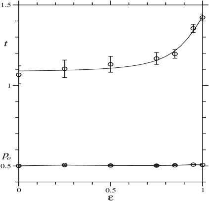
Figure 5: Behavior of $t(\varepsilon)$ and $p_{0}(\varepsilon)$ with $\varepsilon$, when conductances of the initial network are chosen randomly within $(1-\varepsilon,1+\varepsilon)$. Bonds removal is isotropic ($p_{0}$ remains at 0.5).

Next we consider networks from which we removed elements anisotropically. We begin with a square network of unit conductance and remove elements in the horizontal and vertical directions with probabilities $p_{h}=\beta\,p$ and $p_{v}=p$. Analysis of such networks for $\beta=2.0$ using Equation (1) gives $\,p_{0}=0.3383\pm\,0003,\,t=1.3303\pm\,0.0189$. Similarly, for $\beta=1/2\,$, $p_{0}=0.6798\pm\,0.0099,\,t=1.0396\pm\,0.0553$ (See Figure 4). Finite size scaling for the two cases estimates give $t_{FSS}=1.3\pm\,0.10$ and $t_{FSS}=1.05\pm\,0.10$ respectively, in good agreement with Equation (1). The estimates for $p_{0}$ for multiple $\beta$’s, shown in Figure 4, agree with theoretical results for anisotropic networks S. Redner and H. E. Stanley (1979). The value of the critical exponent changes little over the range from $\beta\,>\,1.0\,$ to $\beta\,<\,2.0$.

Now, we consider the slow breaking network process which consist of two subsequent independent random processes, i.e., after a random remotion of conductors; it is imposed to the network remaining elements a conductivity value choosing at random in a range $(1-\varepsilon,1+\varepsilon)$; where $\varepsilon\in\,(0,1)$. Note that, the isotropic case is retrieved for $\varepsilon\,=\,0$. We find that the critical index depends on the value of $\varepsilon$. We conduct our analysis for $\varepsilon=0.00,0.25,\,0.50,\,0.75,\,0.85,\,0.95$ and $1.0$, and at each $\varepsilon$, for network sizes considered earlier. Although the value of the critical point $p_{0}$ is independent of $\varepsilon$ (Figure 5), and the critical exponent increases with $\varepsilon$ (for $\varepsilon\,>\,0.5\,$) (Figure 5), consistent with results for finite size scaling.

Next, we consider networks whose remaining electrical elements randomly degrade as we remove conductances. This problem relate to degradation of porous bone with aging L. Mosekilde (1988). Specifically, we consider networks whose conductance and breakdown decrease by a factor $(1-\alpha\,p)$, where as before, $p$ is the probability for an element to be removed from the network. Once again, as earlier, we analyzed network sizes ranging from $M=20$ to $M=160$ (Figure 6). For $\alpha=1.0$ we find that $p_{0}=0.509\pm\,0.005$, $t=1.287\pm\,0.034,\,a_{1}=-0.123\pm\,0.006\,$ and $\,a_{2}=0.067\pm\,0.003$. The estimated critical exponent using finite size scaling is $t_{FSS}=1.29\pm\,0.10$.

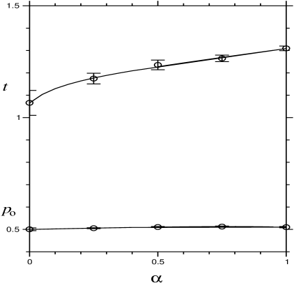
Figure 6: Variations in parameters $t(\alpha)$ and $p_{0}(\alpha)$. When elements are removed from the network with probability $p$, the conductance of those remaining are reduced simultaneously by a factor $(1-\alpha\,p)$. The critical fraction removed elements remain 0.5.

Let us now stress a point on the essential of nonlinear and irreversible properties of the breakdown process. In Figure 7 are shown the strength reduction behavior originated by two different types of damage modalities. As can be seen, both deviates from linearity above the percolation threshold in agreement with M. V. Chubynsky and M. F. Thorpe (2005). The right side of the figure shows the strength reduction behavior for the anisotropic case for $\beta=3.0$. Left side of the figure considers an ensemble of conductor which are randomly removed from the network while their remaining elements are diminished at random by a factor $(1-\,0.75\,p)$. For the slow breaking process, the strength reduction shows a similar behavior.

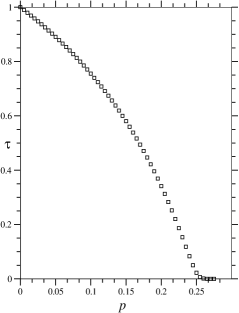
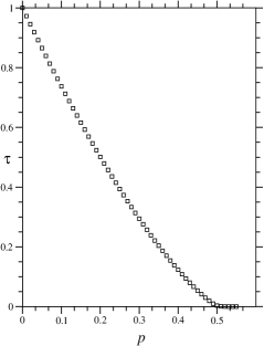
Figure 7: The deviation from linearity of the strength reduction due to the removal of a fraction of conductance in a $160^{2}$ network. The right side shows the anisotropic removal of conductance with probabilities $p$ and $3.0\,p$ in the vertical and horizontal direction.The left side corresponds the case where the elements are randomly removed with probability $p$ meanwhile the ones remaining are simultaneously reduced by a factor $(1-0.75\,p)$.

IV Conclusions

We have computed critical indices for several classes of square networks of conductances using finite size scaling and Equation (1). For the isotropic case, $t=1.066\,\pm\,0.056$ in agreement with the value $t=1.1$ reported by Kirkpatrick S. Kirkpatrick (1978), Straley J. P. Straley (1977a, b), and Stinchcombe and Watson R. B. Stinchcombe and B. P. Watson (1976). However, it is different from the values (close to 1.3) obtained from real space renormalization group methods J. Bernasconi (1976); P. J. Reynolds, W. Klein and H. E. Stanley (1977); D. J. Frank and C. J. Lobb (1988). (This discrepancy has already been discussed by Straley J. P. Straley (1977a).) For anisotropic networks, we compare to an analysis of experimental and computational results by Han, Lee and Lee  K. H. Han, J. O. Lee and Sung-I K Lee (1991) and by Smith and Lobb L. N. Smith and C. J. Lobb (1979). Both groups found that $t=1.3$ when $p=0.33$. Figure 4 shows that for $p=0.33$, the parameter $\beta$ is $1.94$ and $t=1.31$. Further, the values of $p_{0}(\beta)$ for anisotropic removal of conductances (Figure 4) is consistent with theoretical results of Redner and Stanley  S. Redner and H. E. Stanley (1979).

Here, we have presented substantial evidence that critical indices depend on the type of initial network and damage modalities of conductances and the network. Indeed the critical exponent might be a convoluted exponent because of two independent random processes are affecting the strength reduction of networks. Results from previous studies have been shown to be isolated examples of our more general analysis of this problem. It would be of interest to develop a renormalization group based analysis to describe these more general damage processes. We have, thus far, not been successful in identifying such a theory.