Continuum Theory for Piezoelectricity in Nanotubes and Nanowires

Abstract

We develop and solve a continuum theory for the piezoelectric response of one dimensional nanotubes and nanowires, and apply the theory to study electromechanical effects in BN nanotubes. We find that the polarization of a nanotube depends on its aspect ratio, and a dimensionless constant specifying the ratio of the strengths of the elastic and electrostatic interactions. The solutions of the model as these two parameters are varied are discussed. The theory is applied to estimate the electric potential induced along the length of a BN nanotube in response to a uniaxial stress.

Recently there has been interest in the physical properties of materials that are obtained by wrapping a two dimensional lattice to form a one dimensional structure. When the lateral dimensions of the wrapped structure are reduced to the nanometer scale, the new periodicity introduced by this wrapping can have a profound impact on the physical properties of the system. The III-V boron-nitride (BN) exhibits a ground state polarization and a piezoelectric response (electric polarization linearly coupled to an elastic strain) when it is wrapped into a nanotube, although the symmetry of the two dimensional BN sheet permits only a piezoelectric response. This system thus demonstrates the possibility of geometrical control of the piezoelectric response of a nanomaterial, providing a new degree of freedom with significant potential for nanoscale electromechanical applications.

The piezoelectric response of a macroscopic three dimensional system is well described by the continuum Landau Devonshire model Lines and Glass (1977). However, this model does not adequately describe the piezoelectric response of a one dimensional system because the 1D Coulomb kernel is a short range potential (its Fourier transform diverges at small momentum $q$ proportional to $-\log(q)$ rather than as $1/q^{2}$ as in three dimensions). Here we show that this short range kernel leads to new physical effects in $1$D systems such as nanotubes and nanowires. We find that the elastic response of a finite length piezoelectric nanotube to an applied uniform mechanical load is in general spatially nonuniform. The spatial variation of the electric polarization produces a bound charge density that penetrates from the tube end into the interior of the system. In addition, localized surface bound charges develop exactly at the tube ends. The partitioning of the bound charge into its “bulk” and “surface” contribution is then determined by a competition between the electrostatic and elastic interactions in the system. These effects are not described in any simple model for an electrostatic depolarizing field for the tube, as would be possible for three dimensional samples in confined geometries (e.g. spheres, ellipsoids or thin films), and instead require an appropriate continuum theory to study the spatial variation of the electromechanical coupling. In this paper we develop this model and apply it to estimate the magnitude of experimentally accessible electromechanical effects for the case of a BN nanotube.

We consider the effect of an applied mechanical stress on a piezoelectric nanotube with radius $R$ and length $L$. (The generalization to the case of a nanowire with a solid core is straightforward.) A constant stress $\sigma(z)=f$ is applied to the tube and it induces a strain field $\eta(z)$ where $z$ is the coordinate along the tube axis. This strain is linearly coupled to an electric polarization along the tube axis through a piezoelectric constant $e_{s}$, so that $P(z)=e_{s}\eta(z)$. In general an electric polarization of the nanotube can be produced by the uniaxial strain (extension or compression along the tube axis) and by tube torsion. For example, for BN nanotubes the piezoelectric constants that couple to these two elastic strains are determined by the chiral angle that specifies the tube wrapping. For simplicity, in this paper we treat the case where only one elastic degree of freedom is coupled to the polarization. For the BN nanotubes this is realized by “zigzag” tubes that have a nonzero piezoelectric coupling only to uniaxial strain, or for “armchair” tubes that couple only through the tube torsion Sai and Mele (2003).

The free energy of the system can be written as a sum of its bare elastic and electrostatic contributions

$$G=G_{\rm elastic}+G_{\rm electrostatic}-\int_{0}^{L}\eta(z)\sigma(z)\,dz.$$ (1)

Introducing the one dimensional elastic modulus $C_{1}$, the elastic energy is

$$G_{\rm elastic}=\frac{1}{2}C_{1}\int_{0}^{L}\eta(z)^{2}\,dz.$$ (2)

Here $C_{1}=2\pi RC_{2}$ where $C_{2}$ is the elastic modulus for the two dimensional sheet (e.g. $C_{11}$ for a uniaxial strain). $C_{2}$ is the relevant intensive quantity (with units energy/area) that depends on the composition and structure of the tube, and the one dimensional tube modulus $C_{1}$ is an extensive quantity proportional to the tube radius.

Using the piezoelectric constant $e_{s}$ the electrostatic energy can be expressed in terms of the spatial derivatives of the strains as

$$G_{\rm electrostatic}=\frac{e_{s}^{2}}{2}\int_{0}^{L}\int_{0}^{L}\frac{\partial\eta(z)}{\partial z}V(z-z^{\prime})\frac{\partial\eta(z^{\prime})}{\partial z^{\prime}}\,\,dz\,dz^{\prime}.$$ (3)

Here $e_{s}$ is a one dimensional piezoelectric constant giving the strain-induced dipole moment per unit length (with units of charge). For BN nanotubes of moderate radius it can be well approximated using the piezoelectric constant of an infinite two dimensional sheet $e_{2}$ mapped onto the tube circumference Sai and Mele (2003). Thus for most physically relevant situations $e_{s}\approx 2\pi Re_{2}$. $V(z-z^{\prime})$ is a Coulomb kernel describing the electrostatic interaction between rings of charge centered at positions $z$ and $z^{\prime}$ along the tube axis.

It is useful to extract the dimensional dependence of these energies by expressing all lengths in units of the tube radius. Then by introducing the scaled variable $\xi=z/R$, the aspect ratio $\lambda_{1}=L/R$, and another dimensionless parameter $\lambda_{2}=e_{2}^{2}/(RC_{2})$, we have

$$G/(\pi R^{2}C_{2}) = \int_{0}^{\lambda_{1}}[(\eta(\xi))^{2}-2\beta\eta(\xi)]\,d\xi$$ (4)

$$+ {2\pi\lambda_{2}}\int_{0}^{\lambda_{1}}\!\!\!\int_{0}^{\lambda_{1}}\frac{\partial\eta(\xi)}{\partial\xi}V(\xi-\xi^{\prime})\frac{\partial\eta(\xi^{\prime})}{\partial\xi^{\prime}}\,d\xi\,d\xi^{\prime}.$$

Here $\beta=f/(2\pi RC_{2})$ is the equilibrium strain in the absence of any electrostatic coupling. The competition between the electrostatic and elastic effects on the tube is therefore determined by the relative sizes of the scaled lengths $\lambda_{1}$ and $\lambda_{2}$. In the regime where $\lambda_{2}\ll\lambda_{1}$ the electrostatic interactions are negligible, and the equilibrium strain is nearly constant along the length of the tube, albeit with a reduction near the tube ends. Conversely when $\lambda_{2}\gg\lambda_{1}$, the electrostatic interactions dominate and the system seeks to minimize the spatial derivatives of the strain, subject to the constraints of mechanical equilibrium. This leads to a situation where the bound charge density penetrates deep into the tube interior and the applied mechanical stress is nearly completely balanced by the electrostatic interactions. Equation (4) also demonstrates that because of the scaling of the one-dimensional modulus with tube radius, the induced strains are inversely proportional to $R$, i.e. for a fixed aspect ratio large radius tubes are mechanically “stiffer”.

The equilibrium strain field is obtained by minimizing $G$ and satisfies

$$\eta(\xi)=\beta+2\pi\lambda_{2}\int_{0}^{\lambda_{1}}\frac{\partial V(\xi-\xi^{\prime})}{\partial\xi}\frac{\partial\eta(\xi^{\prime})}{\partial\xi^{\prime}}\,d\xi^{\prime}.$$ (5)

Possible stepwise discontinuities of $\eta(z)$ at the sample boundaries can be treated by explicitly writing

$$\frac{\partial\eta(\xi^{\prime})}{\partial\xi^{\prime}}=\eta(0)\delta(\xi^{\prime})-\eta(\lambda_{1})\delta(\xi^{\prime}-\lambda_{1})+\frac{\partial\eta_{i}(\xi^{\prime})}{\partial\xi^{\prime}},$$ (6)

where $\eta_{i}$ denotes the strain field in the sample interior. Then, by integrating Eq. (5) by parts we get

$$\eta_{i}(\xi)=\beta+2\pi\lambda_{2}\int_{0}^{\lambda_{1}}\frac{\partial^{2}V(\xi-\xi^{\prime})}{\partial\xi^{\prime 2}}\eta_{i}(\xi^{\prime})\,d\xi^{\prime}.$$ (7)

In the following we will drop the subscript $i$, and the $\xi^{\prime}$ integrals are understood to extend over the interior of the tube.

The solution of Eq. (7) requires a specification of an appropriate Coulomb kernel $V(z)$. In the simplest continuum model where $V(z)$ describes the interaction of rings of charge, we have

$$V(\xi-\xi^{\prime})=\frac{1}{2\pi}\int_{0}^{2\pi}\frac{d\theta}{\sqrt{(\xi-\xi^{\prime})^{2}+\sin^{2}(\theta)+(1-\cos(\theta))^{2}}}.$$ (8)

This kernel diverges logarithmically at short range. Thus in this model a surface localized bound charge density $\rho(0)\delta(z)$ at the tube end leads to a divergent electrostatic energy. Therefore the boundary condition for the strain field in this model becomes $\eta(0)=\eta(L)=0$. This infinite energy is an artifact of the model and signals a breakdown of the continuum theory at short length scales. To avoid this difficulty, we instead use a “softened” kernel

$$V_{\rm soft}(\xi-\xi^{\prime})=\frac{1}{|\xi-\xi^{\prime}|+\alpha},$$ (9)

which retains the correct long range behavior but remains finite for $\xi\rightarrow\xi^{\prime}$. This softened kernel allows for the presence of a nonzero surface charge density $e_{s}\eta(0)\delta(z)$ at the ends the tube. The value of $\alpha$ determines the energy “cost” of surface charges, and therefore controls the value of $\eta(0)$. Ultimately the distribution of the bound charge into its “surface” and “bulk” contributions is determined by a self consistent solution to the equation of state (7).

Once the equilibrium charge density is determined the electric potential at position $z$ along the tube is obtained by evaluating

$$U(z)=\int_{0}^{L}V(z-z^{\prime})\rho(z^{\prime})\,dz^{\prime}.$$ (10)

After integrating by parts and transforming to scaled variables the potential is expressed

$$U(\xi)=2\pi e_{2}\int_{0}^{\lambda_{1}}\frac{\partial V(\xi-\xi^{\prime})}{\partial\xi^{\prime}}\eta(\xi^{\prime})\,d\xi^{\prime}.$$ (11)

Since the equilibrium condition in Eq. (7) requires that

$$\eta(\xi)-\beta=-\frac{\lambda_{2}}{e_{2}}\frac{\partial U(\xi)}{\partial\xi}$$ (12)

the potential can be expressed as an integral over the strain field $\eta$, and we obtain

$$U(\xi)=\frac{e_{2}}{\lambda_{2}}\int_{\xi}^{\lambda_{1}/2}(\eta(\xi^{\prime})-\beta)\,d\xi^{\prime},$$ (13)

where we have set the electric potential to zero at the center of the tube.

The equilibrium solutions for the strain field $\eta(z)$ (Eq. 7), the bound charge density $\rho=-e_{s}\partial\eta/\partial z$ and the electrostatic potential $U(z)$ (Eq. 13) are displayed in Fig. (1) for the model in the regime where the elastic interactions dominate ($\lambda_{2}\ll\lambda_{1}$) and in Fig. (2) for the regime where the electrostatic interactions dominate ($\lambda_{1}\ll\lambda_{2}$). The softened kernel was used with $\alpha=.001$. The data in these plots was obtained by finite element analysis. The tube length was divided into $1000$ unequally spaced bins ($1/3$ evenly spaced in the first $10\%$ of the tube, $1/3$ evenly spaced in the last $10\%$, and $1/3$ evenly spaced across the middle $80\%$ of the tube). Bin number was increased in steps of $100$ until successive solutions differed by less than $1.2\%$. The slowest convergence occurs at the end of the tubes, with the solution differing by less than $.2\%$ on the last iteration over the middle $99.8\%$ of the tube.

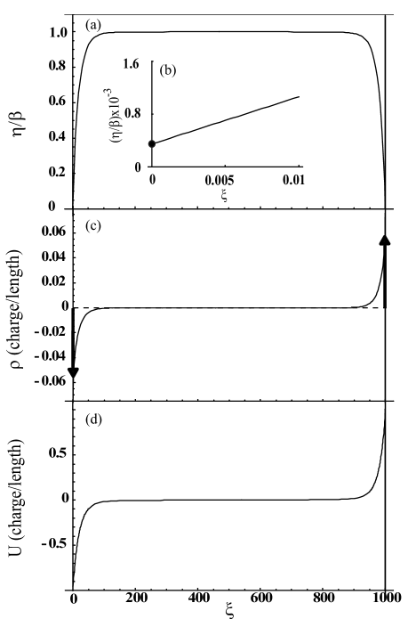
Figure 1: Equilibrium solutions for a piezoelectric tube in the elastically dominated limit. (a) Equilibrium strain profile from Eq. (7). The strain is well approximated by the elastic limit over most of the tube. (b) Inset, strain value at tube boundary. Notice $\eta(0)\not=0$ with our choice of $V$. (c) The bound charge density, $\rho=-e_{s}\partial\eta/\partial z$. The arrows represent delta functions in the charge density. (d) Equilibrium potential from Eq. (13). The graphs were generated using $\beta=1$, $\lambda_{1}=1000$, $\lambda_{2}=10/\pi$, and $e_{s}=1$ (charge).

In the elastically dominated limit, the equilibrium strain is nearly constant in the interior region of the tube where $\eta\approx\beta$. The electrostatic interactions effectively increase the elastic moduli near the surface region, leading to a suppression of the strain. This suppression implies a spatial variation of the polarization and a volume bound charge density that is obtained self consistently by solving Eq. (7). Finally, we see that the equilibrium strain is in general nonzero at the tube ends. Thus, in addition to the continuous volume bound charge density, a true surface localized bound charge is obtained at the terminations. In a long (semi-infinite) tube the equilibrium strain asymptotically relaxes to its elastic limit following a power law, e.g. $1-\eta(\xi)/\beta\propto(\gamma/\xi)^{2}$ where $\gamma=\sqrt{2\pi\lambda_{2}}$. The distribution of the bound charge is plotted in the central panel, which shows that the main effect of the electrostatic interaction is to “spread” the bound charge density near the tube ends. In the elastically dominated limit most of the potential drop across the tube, shown in Fig. (1-d), occurs in the regions near the tube ends.

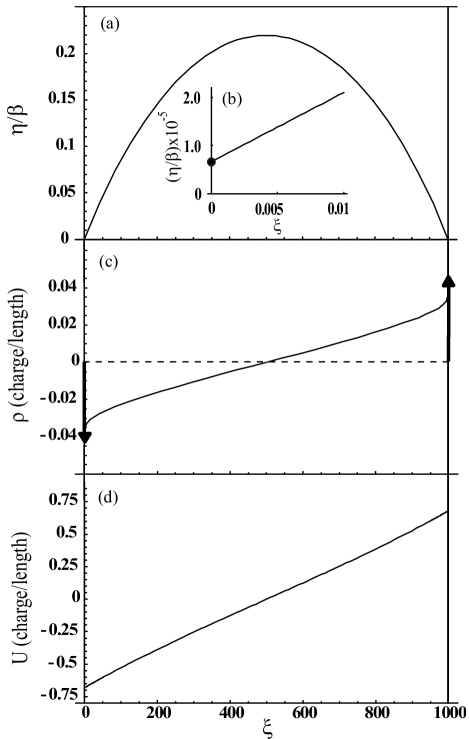
Figure 2: The equilibrium solutions for a piezoelectric tube in the electrostatically dominated limit. (a) Equilibrium strain profile from Eq. (7). Notice that the maximum value of the strain is about 1/5 of the elastic limit. (b) Inset, strain value at tube boundary. Notice $\eta(0)\not=0$ with our choice of $V$. (c) The bound charge density, $\rho=-e_{s}\partial\eta/\partial z$. The arrows represent delta functions in the charge density. (d) Equilibrium potential from Eq. (13). The graphs were generated using $\beta=1$, $\lambda_{1}=1000$, $\lambda_{2}=10000/\pi$, and $e_{s}=32$ (charge).

This behavior is contrasted with the situation for the electrostatically dominated limit shown in Fig. (2). In this regime, the system seeks to reduce its strain gradients subject to the constraint of mechanical equilibrium. This leads to a state in which the bound charge extends along the entire length of the tube. The numerical solution for the equilibrium strain shown in Fig. (2-a) is reasonably well approximated using only the lowest allowed Fourier component with the ends of the tube clamped. The overall magnitude of the strain is also strongly reduced, since it is limited by the electrostatic coupling strength instead of the bare elastic constant. The bound charge density vanishes at the center of the tube by symmetry and varies approximately linearly as a function of position, with logarithmic corrections close to the ends of the tube. Interestingly, Eq. (12) requires that the electric potential is a linear function of position in the limit that $\eta(z)\ll\beta$, as is shown in Fig. (2-d).

Since the one dimensional Coulomb kernel is a short range interaction it is useful to consider the limit where the kernel is a contact interaction $V(\xi-\xi^{\prime})=\delta(\xi-\xi^{\prime})$. Then the free energy in Eq. (4) reads

$$G/(\pi R^{2}C_{2})=\int_{0}^{\lambda_{1}}\!\!\left[(\eta(\xi))^{2}-2\beta\eta(\xi)+2\pi\lambda_{2}\left(\frac{\partial\eta(\xi)}{\partial\xi}\right)^{2}\right]\,d\xi.$$ (14)

Up to an additive constant, this describes the free energy of a superconducting disk, with penetration depth $\sqrt{2\pi\lambda_{2}}$ immersed in a perpendicular field $H_{0}=-\beta$. The equilibrium solution to this model is obtained analytically as

$$\eta(\xi)=\beta\left(1-\frac{\cosh((\xi-\lambda_{1}/2)/\sqrt{2\pi\lambda_{2}}\,)}{\cosh((\lambda_{1}/2)/\sqrt{2\pi\lambda_{2}}\,)}\right).$$ (15)

Thus the strain profile in the elastically dominated limit shown in Fig. (1-a) give the piezoelectric analog to the Meissner expulsion of an applied field (stress) and the electrostatic regime of Fig. (2-a) corresponds to the limit of a small superfluid density where the penetration depth is of order the length of the system. For the contact interaction model the induced potential is simply proportional to the bound charge density, so that a measurement of the spatial variation of the potential probes the piezoelectric analog of the London penetration depth. Note however that the physical kernel retains an asymptotic $1/\xi$ tail leading to a power law decay of the strain field.

Recently, BN nanotubes were predicted to exhibit a significant piezoelectic response Mele and Kral (2002); Nakhmanson et al. (2003). Here we predict the piezoelectric response of a “zigzag” BN nanotube under uniform longitudinal tensile or compressive stress. The 2D elastic constants for various chiral BN tubes were calculated in Ref. Hernández et al., 1998; here we use an average value of $C_{2}=.30$ TPa  nm . Ref. Sai and Mele, 2003 gives the piezoelectric constant for a BN sheet as $e_{2}=.12$ e/Bohr. Experimentally accessible forces are on the nano-Newton scale; we arbitrarily assume a force of $1$ nN. Typical tube dimensions are $R=1$ nm and $L=1$ $\mu$m.

Using these values we find that $\lambda_{1}=1000$, $\lambda_{2}=4.4\times 10^{-3}$, and $\beta=5.3\times 10^{-4}$. These values give an asymptotic decay constant of $\gamma=.17$, and the strain to relaxes to its elastic limit very quickly. Our numerical solution shows the equilibrium strain is within $1\%$ of the elastic limit at a depth of $3R$. Thus the bound charge density, although continuous, barely penetrates the bulk of the tube, and the entire potential drop occurs near the ends. Applying the continuum theory to this system and converting to SI units we obtain an estimate of $.48$ V across the tube for an applied tension $f=1\,{\rm nN}$. It would be interesting to experimentally measure this strain induced electrostatic potential and to resolve its spatial variation near the tube ends using scanning probe potentiometry.

The theory for a solid core nanowire follows the same formalism, but unlike the nanotube, in a nanowire the corresponding $\lambda_{2}$ is fixed entirely by the material parameters, independent of $R$. This occurs for a nanowire because the extensive variables, $e_{s}$ and $C_{1}$, are proportional to the cross-sectional area rather than the circumference. They are related to the relevant intensive variables by $e_{s}=\pi R^{2}e_{3}$ (where $e_{3}$ is the 3D piezoelectric constant in units of charge/area) and $C_{1}=\pi R^{2}C_{3}$ (where $C_{3}$ is the 3D elastic constant in units of pressure). The equilibrium strain then satisfies Eq. (7) with $\lambda_{2}=e_{3}^{2}/(2C_{3})$ and $\beta=f/(\pi R^{2}C_{3})$. Thus two nanowires with the same aspect ratio but different radii will have the same scaled strain, $\eta/\beta$, unlike hollow nanotubes where larger radius tubes have smaller $\lambda_{2}$ and thus are elastically dominated.

This work was supported by the Department of Energy under grant DE-FG$02$-ER$0145118$ and by the National Science Foundation under grant DMR-$00$-$79909$.

References

- Lines and Glass (1977) M. E. Lines and A. M. Glass, Principles and Applications of Ferroelectics and Related Materials (Clarendon Press, Oxford, 1977).
- Sai and Mele (2003) N. Sai and E. J. Mele, Phys. Rev. B 68, 241405 (2003).
- Mele and Kral (2002) E. J. Mele and P. Kral, Phys. Rev. Lett. 88, 056803 (2002).
- Nakhmanson et al. (2003) S. M. Nakhmanson, A. Calzolari, V. Meunier, J. Bernholc, and M. B. Nardelli, Phys. Rev. B 67, 235406 (2003).
- Hernández et al. (1998) E. Hernández, C. Goze, P. Bernier, and A. Rubio, Phys. Rev. Lett. 80, 4502 (1998).