Address for correspondence:] Max Planck Institute for Biochemistry, Dept. of Molecular Structural Biology, Am Klopferspitz 18a, 82152 Martinsried (Munich), Germany. Fax n.: +49 (89) 85782641.

THEORETICAL STUDY OF COMB–POLYMERS ADSORPTION ON SOLID SURFACES

ABSTRACT

We propose a theoretical investigation of the physical adsorption of neutral comb–polymers with an adsorbing skeleton and non–adsorbing side–chains on a flat surface. Such polymers are particularly interesting as ”dynamic coating” matrices for bio–separations, especially for DNA sequencing, capillary electrophoresis and lab–on–chips. Separation performances are increased by coating the inner surface of the capillaries with neutral polymers. This method allows to screen the surface charges, thus to prevent electro–osmosis flow and adhesion of charged macromolecules (e.g. proteins) on the capillary walls. We identify three adsorption regimes: a ”mushroom” regime, in which the coating is formed by strongly adsorbed skeleton loops and the side–chains anchored on the skeleton are in a swollen state, a ”brush” regime, characterized by a uniform multi–chains coating with an extended layer of non–adsorbing side–chains and a non–adsorbed regime. By using a combination of mean field and scaling approaches, we explicitly derive asymptotic forms for the monomer concentration profiles, for the adsorption free energy and for the thickness of the adsorbed layer as a function of the skeleton and side–chains sizes and of the adsorption parameters. Moreover, we obtain the scaling laws for the transitions between the different regimes. These predictions can be checked by performing experiments aimed at investigating polymer adsorption, such as Neutron or X-ray Reflectometry, Ellipsometry, Quartz Microbalance, or Surface Force Apparatus.

I Introduction

Polymer adsorption on surfaces is of paramount importance for numerous applications. In material sciences, it is used to control surface properties such as wetting, hardness, or resistance to aggressive environments. It can also have detrimental effects in fouling, alteration of the aspects of materials, and generally speaking unwanted changes in surface properties.

Polymer adsorption also gains more and more attention in the field of biology, in which it plays an essential role in bio–compatibility, cell adhesion, containers and instruments contamination, and in bio–analytical methods. Many proteins, in particular, have a strong amphiphilic character, and tend to adsorb easily to surfaces bearing charges or hydrophobic domains. Strong efforts have been continuously made in the last 20 years, to develop surface treatments able to prevent unwanted adsorption of biomolecules in a water environment. The proposed solutions often amount to treat the surface with specially chosen proteins, oligomers or polymers. In most cases, a very hydrophilic polymer is required. Numerous polymers have been proposed in this context, including polysaccharides, Polyvinyl–alcohol, and the very popular Polyethyleneoxide.

Depending on the application, two different approaches can be envisaged: either polymer grafting onto the surface by one or several covalent bonds (see e.g. Hjerten and Kubo (2000) etc…), or spontaneous adsorption. The latter solution is in general easier to implement, and the regeneration of a fouled or damaged surface is easier. However, the adsorbed polymer layer is in general more fragile than a covalently bonded surface, and the adsorption approach puts constraints on the chemical nature and architecture of the polymers, that can be difficult to fulfill. In particular, surface coatings in the field of biology must in most cases be hydrophilic. Since very hydrophilic polymers most often do not adsorb spontaneously onto surfaces in a water environment (their free energy in the solvated state is very low), some ”tricks” must be developed.

One efficient way to favor adsorption of a hydrophilic layer is to use block copolymers, with one (or several) hydrophilic block, and one or several blocks playing the role of an anchor. In particular, diblock and triblock copolymers or oligomers, such as alkyl–Polyethyleneoxide diblocks, or Polyethyleneoxide–Polypropyleneoxide–Polyethyleneoxide triblocks, were used with success for several applications. They are far to be a universal solution to unwanted adsorption and wall–interactions of biomolecules. In particular, they seem rather unsuccessful in the field of capillary electrophoretic separations.

This bio–analytical method has been widely popularized by the large genome projects (the human genome project, and most of the current genome projects rely mainly on capillary array electrophoresis for DNA sequencing Marshall and Pennisi (1998)) and its importance is bound to increase further with the development of massive ”post–genome” screening and ”lab–on–chips” methods for research and diagnosis Salas-Solano et al. (2000); Carrilho (2000). In capillary electrophoresis, analytes are separated by electrophoretic migration under a high voltage (typically 200 to 300 V/cm) in a thin capillary (typically 50 $\mu$m ID). Interactions of the analytes with the walls is of paramount importance, because it can lead to considerable peak trailing and because of electro–osmosis, a motion of the fluid induced by the action of the electric field on the excess of mobile free charges in the vicinity of a charge surface (see e.g. Viovy (2000)).

Consider an infinitely long pipe filled with an electrolyte, with a non–vanishing Zeta potential (the most common situation when a solid is in contact with an electrolyte). The surface has a net charge and a Debye layer of counterions forms in the fluid in the vicinity of this surface in order to minimize the electrostatic energy. In buffers typically used in electrophoresis, the Debye layer has a thickness of a few nanometers. Choosing for definiteness a negatively charged surface, such as e.g. glass in the presence of water at pH 7, the Debye layer is positively charged. Applying an electric field along the pipe, the portion of fluid contained in the Debye layer is dragged towards the cathode. Solving the Stokes equation with the boundary condition of zero velocity at the surface leads to a ”quasi–plug” flow profile, with shear localized within the Debye layer and a uniform velocity in the remainder of the pipe. If the electrical charge on the surface is non–uniform, due for example to a local adsorption of biopolymers, the velocity at the wall, which is imposed by the local zeta potential, is also non–uniform. In such case, the flow is no more a plug flow, and there are hydrodynamic recirculations detrimental to the resolution Ajdari (1995). Electro–osmosis generally has very dramatic consequences on the performance of practical electrophoretic separations, and it must be thoroughly controlled. Polymers at the interface can play a double role in circumventing electro–osmosis: by preventing unwanted adsorption of analytes or impurities contained in the electrophoretic buffer, and by decoupling the motion at the wall from the motion of the bulk fluid. For this, the polymer layer must be thicker than the Debye length. Different strategies, using either covalently bonded polymers (see e.g. Horvath and Dolnik (2001)) or reversibly adsorbed polymers (so called ”dynamic coating”, see e.g. Righetti et al. (2001); Doherty et al. (2002)), have been developed. The use of relatively short copolymers Liang et al. (2001); Liang and Chu (1998) has been rather deceptive, probably because they lead to rather thin layers, and because the adsorption free energy of an individual chain is too low to resist the rather aggressive conditions encountered during electrophoresis in strong fields (in particular high shear at the wall). These oligomers need to be present in the solution at a high concentration, in order to yield sufficient dynamic coating. Presently, the most efficient applications of dynamic coating have involved Poly–Dimethyl Acrylamide (PDMA) Madabhushi (1998) or copolymers of this polymer with other acrylic monomers Chiari et al. (2000). This polymer seems to present an interesting affinity to silica walls, thanks to the presence of hydrogen bonding, while remaining soluble enough in water to behave as a sieving matrix. It was demonstrated Albarghouthi et al. (2001), however, that its reduced hydrophilicity as compared with, e.g. Acrylamide Zhou et al. (2000), results in poorer separation performance, probably due to increased interactions with the analytes.

Recently, we proposed Barbier et al. (2002) a new family of block copolymers comprising a very hydrophilic Poly–Acrylamide (PA) skeleton and PDMA side–chains, as dynamic coating sieving matrices for DNA electrophoresis. These matrices provide an electro–osmosis control comparable to that of pure PDMA, while allowing for better sieving. A large range of different microstructures can be conceived and constructed, varying the length and chemical nature of the grafts and of the skeleton, and the number of grafts per chain. The aim of the present article is to investigate theoretically the adsorption mechanisms and the structure of adsorbed layers of polymers with this type of microstructure, in order to better understand the properties, and to provide a rational basis for further experimental investigations and applications. The adsorption of homopolymers, of di- or triblock copolymers, and random copolymers of adsorbing and non–adsorbing polymers, has been investigated theoretically Joanny and Johner (1996); Semenov et al. (1996, 1998); Marques and Joanny (1989); Johner and Joanny (1997); Gennes (1981); de Gennes (1980); Marques and Joanny (1990); Marques et al. (1988). To our knowledge, however, the case of a comb–polymer with different adsorption properties on the skeleton and on the grafts has never been considered. We address this problem here, generalizing on previous work on random and triblock copolymers.

The architecture of the paper is as follows: In Section II we investigate the adsorption of comb–polymers with adsorbing backbone and non-adsorbing side–chains. In Section II.1 we present a mean field model for the analysis of the adsorption of combs in the limit of small side–chains, i.e. in the mushroom regime ($N_{t}\ll N_{B}$ , where $N_{t}$ and $N_{B}$ are the number of monomers of a non–adsorbing side–chain and of the corresponding adsorbing backbone chain section, respectively).

In Section III, we use a scaling approach to describe the adsorption of comb–polymers both in the mushroom and in the brush regime (i.e. in the limit of large side–chains) and the cross–over between these two regimes.

II Adsorption of Comb–Polymers with Adsorbing Backbone and non–Adsorbing Side–Chains: Mean Field Theory

In this section we give a mean field description of the adsorption of comb–polymers with adsorbing backbone and non–adsorbing side–chains onto a flat solid substrate. The combs have an adsorbing backbone B, made of p blocks of $N_{B}$ monomers each with gyration radius $R_{B}\sim a\,N_{B}^{1/2}$, on which are grafted $p$ non–adsorbing T side–chains, of $N_{t}$ monomers each and of gyration radius $R_{t}\sim a\,N_{t}^{1/2}$, where $a$ is the monomer size. We study the adsorption behavior of combs, which is monitored by the mass ratio between the adsorbed backbone B and the non–adsorbing side–chains T.

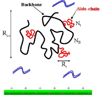
Figure 1: Comb–copolymer in solution, made of an adsorbing backbone made of $p$ blocks of $N_{B}$ monomers each and with $p$ non–adsorbing side–chains of $N_{t}$ monomers each. The total number of monomers is $N=p\,(N_{B}+N_{t})$ (with $p=3$), and the gyration radius $R_{\rm co}\sim a\,N^{1/2}$, $a$ being the monomer size.

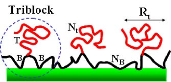
Figure 2: Mushroom configuration for a comb–polymer, made out of $p$ ($p=3$) triblock sub–units. Each triblock is made of $2$ backbone blocks of $N_{B}/2$ monomers and of one anchored side–chain of $N_{t}$ monomers and gyration radius $R_{t}$ (indicated in the Figure with the letters $B$ and $T$, respectively).

We treat at the mean field level the case of small side–chains and low grafting density. This leads to a “mushroom” configuration for the adsorbed comb–polymers, having the backbone adsorbed on the surface and the side–chains dangling from the backbone, with weak steric interaction between them (see Fig.1). Our analysis is based on the idea of describing the combs as linear chains having ’triblock copolymers’ as renormalized monomers (see Fig.2). By exploiting the known solution for linear chains adsorbing from a dilute solution on a flat surface, one can directly derive the comb–polymers adsorption profile, by integrating out the triblock copolymers degrees of freedom.

II.1 Mean Field Theory of Triblock Copolymer Adsorption

Consider a dilute solution of triblock copolymers (p=1), with an adsorbing backbone made of two large adsorbing blocks of $N_{B}/2$ monomers each, and one non–adsorbing small side–chain, of $N_{t}$ monomers, with $N_{B}\gg N_{t}$. The total number of monomers is $N=N_{B}+N_{t}\sim N_{B}$. We solve the problem in the Ground State Dominance Approximation, applicable to the case where the polymers have large enough molecular weights and there is only one bound state of energy $E_{o}<0$. A detailed description of the triblock copolymer adsorption behavior and configurations can be obtained by deriving the polymer partition function $Z_{N}(z)$, in the case where one backbone end–point is fixed at position $z$ above the adsorbing surface ($z=0$) and the other end–point is free. The partition function $Z_{n}(z)$ is a solution of the so–called Edwards equation Semenov et al. (1998); Joanny and Johner (1996):

$$\left\{\begin{array}[]{lll}-\displaystyle{\frac{\partial Z_{n}(z)}{\partial n}}&=&-\displaystyle{\frac{\partial^{2}Z_{n}(z)}{\partial z^{2}}}\,+\,U(z)\,\,Z_{n}(z),\\ \\ \left.-\displaystyle{\frac{\partial\ln Z_{n}(z)}{\partial z}}\right|_{z=0}&=&-\displaystyle{\frac{1}{b}},\end{array}\right.$$ (1)

where the unit length has been defined as $a/\sqrt{6}$ and $a$ is the monomer size. The boundary condition imposed at the surface is a good approximation of the surface potential effect, if we neglect the details of the concentration profile close to the surface. The extrapolation length $b$ gives a measure of the strength of the adsorption. We build here the partition function of the adsorbed combs starting from the known solution $Z^{o}_{N}(z)$ for the adsorption of a linear chain of $N$ monomers, which is also a solution of Eq.(1). Far from the surface the chain is free and can assume all configurations in space, $Z^{o}_{N}(z\gg R_{B})=1$. We choose the normalization of the partition function to be one when the chain reduces to one monomer, $Z^{o}_{0}(z)=1$.

The mean field effective potential experienced by the adsorbed chains can be expressed self–consistently as:

$$U(z)\;=\;\Phi(z)\,-\,\Phi_{b}\;=\;v\,(c(z)-c_{b}),$$ (2)

where $\Phi(z)$ is the monomer volume fraction, equal to the bulk value $\Phi_{b}$ sufficiently far from the surface, $v$ is the excluded volume parameter ($v\sim a^{3}>0$ in a good solvent) and $c(z)$ is the monomer concentration.

The partition function $Z^{o}_{N}$ can be split into two contributions: the adsorbed states contribution $Z_{N}^{o^{a}}$, arising from chains having at least one monomer adsorbed onto the surface, and a free chain contribution $Z_{N}^{o^{f}}$, arising from chains with no adsorbed monomers, so that $Z^{o}_{N}=Z_{N}^{o^{a}}+Z_{N}^{o^{f}}$. We can derive an expression for both components as independent solutions of the Edwards equation, with appropriate boundary conditions (see Section II.2). Starting from the knowledge of $Z_{N}^{o^{a}}$ and of $Z_{N}^{o^{f}}$ (which from now on we denote as $Z_{N}^{o}$ and $Z_{N}^{f}$) for the adsorption of a linear chain of $N$ monomers, we build the partition function of a triblock copolymer, by neglecting the effect of free triblock copolymer chains on the adsorption profile near the surface. The non–adsorbing side–chains contribute as a small perturbation to the adsorption profile.

II.2 Backbone Partition Function

For the adsorption of a linear backbone, made of $N_{B}$ monomers, the Ground State Dominance Approximation amounts to considering the limit of very large molecular weights, $\epsilon_{o}\,N_{B}\gg 1$, where $\epsilon_{o}$ is the absolute value of the contact free energy per monomer ($\epsilon_{o}=|E_{0}|=-E_{0}$). This implies that the expansion of $Z_{N_{B}}^{o}(z)$ in terms of the normalized eigenvectors $\psi_{i}(z)$ ($\int_{0}^{\infty}\;{\rm d}z\,\psi_{i}\,\psi_{j}\,=\,\delta_{ij}$) and of the eigenvalues of Eq.(1) is dominated by the first ground state term:

$$Z_{N_{B}}^{o}(z)\quad\sim\quad\sum_{i}\,k_{i}\;\psi_{i}(z)\,e^{\epsilon_{i}\,N_{B}}\quad\sim\quad k_{o}\;\psi_{o}(z)\,e^{\epsilon_{o}\,N_{B}}\,+\,...\qquad\epsilon_{o}\,N_{B}\gg 1,$$ (3)

where $\psi_{o}$ is a solution of:

$$\begin{array}[]{lll}0&=&-\displaystyle{\frac{\partial^{2}\psi_{o}(z)}{\partial z^{2}}}\,+\,(U(z)+\epsilon_{o})\,\,\psi_{o}(z),\end{array}$$ (4)

with boundary condition:

$$\begin{array}[]{lll}\displaystyle{\frac{-1}{b}}&=&\left.\displaystyle{\frac{1}{\psi_{o}}\,\frac{\partial\psi_{o}}{\partial z}}\right|_{z=0}\qquad{\rm and}\qquad\psi_{o}(z\rightarrow\infty)\,=\,0.\end{array}$$ (5)

The amplitude $k_{o}$ is fixed by imposing the backbone end–points conservation relation (see also Grosberg and Khoklov (1994)):

$${\frac{\Gamma_{o}}{N_{B}}}\quad=\quad\displaystyle{\int_{0}^{\infty}}\,\displaystyle{\frac{\rho_{e}(z)}{2}}\;{\rm d}z,$$ (6)

where the parameter $\Gamma_{o}$ represents the surface coverage (number of monomers per unit surface) and $\rho_{e}(z)$ is the end–points monomer density. Close to the surface, the end–points density $\rho_{e}(z)$ is proportional to the total partition function of the linear backbone, $\rho_{e}(z)\simeq 2\;\Phi_{b}\;Z^{o}_{N_{B}}(z)/N_{B}$. The adsorbance $\Gamma_{o}$ is directly obtained by integrating the monomer volume fraction $\Phi(z)$, which can be expressed as the sum of the loops and of the dangling tails contribution, $\Phi(z)=\Phi_{\ell}(z)\,+\,\Phi_{t}(z)$, with:

$$\Phi_{\ell}(z)\,=\,\displaystyle{\frac{\Phi_{b}}{N_{B}}}\,\displaystyle{\int}Z^{o}_{N_{B}-n}(z)\,Z^{o}_{n}(z)\,dn,$$ (7)

giving $k_{o}=\int\,\psi_{o}$, $\Phi_{\ell}\sim\Gamma_{o}\,\psi_{o}^{2}$ and $\Gamma_{o}=\Phi_{B}\,k_{o}^{2}\,e^{\epsilon_{o}\,N_{B}}$.
By taking into account the contributions of the free dangling backbone ends, one can define the order parameter $\varphi(z)\;\sim\;\int\;Z^{f}_{n_{B}}(z)\;e^{-\epsilon_{o}\,n_{B}}\;dn_{B},$ which is solution of the following equation:

$$\begin{array}[]{lll}1&=&-\displaystyle{\frac{\partial^{2}\varphi(z)}{\partial z^{2}}}\,+\,(U(z)+\epsilon_{o})\,\,\varphi(z),\end{array}$$ (8)

derived from Eq.(1) for $Z_{n_{B}}^{f}(z)$, with boundary condition $\varphi(0)\,=\,0$. One can solve the differential equations for $\psi_{o}(z)$ and $\varphi(z)$ and express the effective potential $U$ (or equivalently the monomers volume fraction $\Phi$ in the case of dilute solutions) as:

$$\Phi\quad=\quad\Phi_{\ell}\,+\,\Phi_{t}\quad=\quad\Gamma_{o}\,\psi_{o}^{2}\,+\,B_{o}\,(\sqrt{\Gamma_{o}}\,\psi_{o})\,\varphi,$$ (9)

where:

$$\begin{array}[]{lll}\sqrt{\Gamma_{o}}\,\psi_{o}&=&\left\{\begin{array}[]{l}\sqrt{2}\quad(z+b)^{-1}\qquad 0<z<z^{*}\\ \sqrt{2}\;(N_{B}\,b)\quad z^{-4}\qquad z^{*}<z<\lambda_{o},\end{array}\right.\\ \\ \varphi&=&\left\{\begin{array}[]{l}z^{2}/3\;\log(z/z^{*})\qquad 0<z<z^{*}\\ z^{2}/18\qquad z^{*}<z<\lambda_{o},\end{array}\right.\end{array}$$ (10)

with $z^{*}\sim(N_{B}\,b\cdot\ln(N_{B}/b^{2}))^{1/3}$, $\Gamma_{o}\sim 2/b$, $k_{o}=\sqrt{2/\Gamma_{o}}\;\log(z^{*}/b)\sim 1/3\,\sqrt{b}\;\log(N_{B}/b^{2})$ and $B_{o}=2\,\sqrt{\Gamma_{o}}/(N_{B}\,k_{o})$. The value $\epsilon_{o}$ of the ground state energy can be expressed as:

$$\begin{array}[]{lll}\epsilon_{o}&=&\displaystyle{\frac{1}{N_{B}}}\;\ln\left[\displaystyle{\frac{\Gamma_{o}}{\Phi_{B}\;k_{o}^{2}}}\right]\quad\sim\quad\displaystyle{\frac{1}{N_{B}}}\;\ln\left[\displaystyle{\frac{2}{\Phi_{B}\,b^{2}}}\right],\end{array}$$ (11)

The parameter $\lambda_{o}\sim\epsilon_{o}^{-1/2}$ is the average thickness of the adsorbed layer.

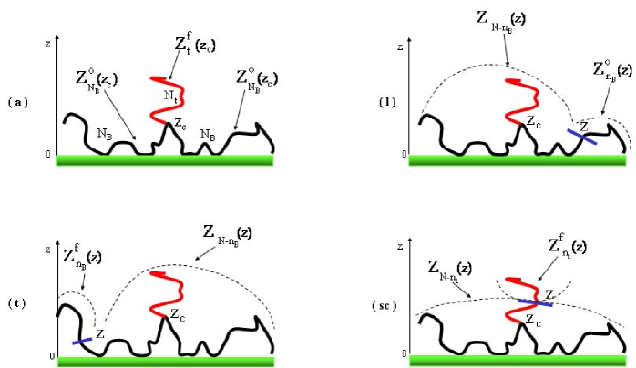
Figure 3: Representation of the construction of the triblock total partition function $Z$ (a) and of the (l) backbone’s loops (l) tails (t) and side–chains (sc) contributions to the triblock copolymer monomer volume fraction $\Phi^{\rm TB}$, starting from the knowledge of the partition functions for the adsorbed backbone blocks, $Z^{o}$ and for the dangling tails, $Z^{f}_{t}$ ($z_{c}$ is the triblock’s core position above the adsorbing surface).

The non–adsorbing side–chain states are described by the “free states” function $Z^{f}_{N_{t}}(z)=Z_{t}^{f}(z)$ (with $Z^{f}_{t}(z=0)=0$ and $Z^{f}_{t}(z\rightarrow\infty)=1$) of a linear non–adsorbed chain of $N_{t}$ monomers, with the constraint of having one end–point anchored at the middle of the adsorbing backbone at $z=z_{c}$, the other end point being integrated out (see Fig.3). The non–adsorbing side–chains feel a strong entropic repulsion at the surface within a layer of thickness $R_{t}\,\sim\,a\,N_{t}^{1/2}$, where $R_{t}$ is their radius of gyration. Thus, for $0\,\leq z\leq\,R_{t}$, the probability of finding “free” side–chains is very low, $Z_{t}^{f}(z)\ll 1$, while for $z>R_{t}$ one has $Z_{t}^{f}(z)\sim 1$. A detailed calculation of the propagator and of the partition function of free chains is given in Appendix C assuming that the side chains only give a small contribution to the total concentration profile; for simplicity, we only give here scaling arguments.

Close to the surface, the most important contribution to the adsorption profile comes from the central monomers of the side–chains Semenov et al. (1998), meaning that $Z_{t}^{f}(z)\sim\psi^{f}(z)$, where $\psi^{f}(z)$ describes ’free’ (non–adsorbing) states and satisfies the same equation as $\psi_{o}(z)$, but with different boundary conditions at the surface, $\psi^{f}(0)\,=\,0$. For $0\leq z\leq R_{t}$, one can express $\psi^{f}(z)$ as a function of $\psi_{o}(z)\sim 1/z$, $\psi^{f}(z)\,=\,\psi_{o}\,\displaystyle{\int_{d}^{z}}\,\psi_{o}^{-2}\;{\rm d}z\,\sim\,z^{2}$, so that:

$$\psi^{f}(z)\,\sim\,\left\{\begin{array}[]{ll}\displaystyle{\frac{z^{2}}{R_{t}^{2}}}&z\leq R_{t},\\ 1&R_{t}<z\leq\lambda_{o}.\end{array}\right.$$ (12)

II.3 Triblock Copolymer Partition Function

We now derive the triblock copolymer partition function $Z_{N}(z)\sim k^{\prime}\,\psi_{o}(z)\,e^{\epsilon\,N_{B}}$ (where $k^{\prime}$ is a constant to be determined and $\epsilon$ is the adsorption energy per monomer of the triblock, with $\epsilon\,>\,\epsilon_{o}$) by proceeding analogously to the case of a linear chain and taking into account the constraint of having a non–adsorbing side–chain anchored at the mid–point of the adsorbing backbone. We start by deriving the total partition function for a triblock copolymer, which is built from the knowledge of the linear backbone partition function $Z^{o}_{N_{B}/2}$ and the partition function of the anchored side–chains $Z^{f}_{t}$:

$$Z\quad=\quad\int_{0}^{+\infty}\,{\rm d}z_{c}\,\int_{0}^{+\infty}\,{\rm d}z\;\;Z^{o}_{N_{B}/2}(z,z_{c})\;Z^{f}_{t}(z_{c})\;Z^{o}_{N_{B}/2}(z_{c})\;=\;Z^{o}\;\;\displaystyle{\frac{e^{(\epsilon-\epsilon_{o})\,N_{B}}}{\Gamma_{o}\,R_{t}}},$$ (13)

where $z_{c}$ is the vertical coordinate of the core (i.e. the side–chain anchoring point) above the surface (see Fig.2), $Z^{o}_{N_{B}/2}(z,z_{c})=\psi_{o}(z)\,\psi_{o}(z_{c})\,e^{\epsilon\,N_{B}/2}$ is the partition function of an adsorbing backbone block with one end at $z_{c}$ and one end at $z$, $Z^{f}_{t}(z_{c})$ is the partition function of the non–adsorbing side–chains with one end at $z=z_{c}$ and $Z^{o}=k_{o}^{2}\,e^{\epsilon_{o}\,N_{B}}$. By combining the classical chemical potential balance for a triblock and a linear chain ($\Phi_{b}/N=\Gamma/(N\,Z)$) one obtains:

$$\ln\left(\frac{\Gamma}{\Gamma_{o}}\right)-N_{B}\,(\epsilon-\epsilon_{o})\,+\,\ln(\Gamma_{o}\,R_{t})\,=\,0$$ (14)

Assuming again that the side–chains give only a small perturbation to the total concentration in the adsorbed layer, one can approximate the triblock copolymer surface coverage $\Gamma$ by the linear chain surface coverage, $\Gamma\sim\Gamma_{o}$, leading to the following expression for the triblock copolymer ground state energy:

$$\epsilon\quad=\quad\epsilon_{o}\,+\,\displaystyle{\frac{1}{N_{B}}}\ln(\Gamma_{o}\,R_{t}).$$ (15)

The density of junction points of a triblock copolymer at position $z_{c}$ above the adsorbing surface can be built using similar arguments to those used for the total partition function. Starting from the single chain partition functions $Z^{f}_{t}$ and $Z^{o}_{N_{B}/2}$, $\rho^{\rm TB}_{\rm c}(z_{c})\,=\,\Phi_{b}\,Z^{f}_{t}(z_{c})\cdot Z^{o^{2}}_{N_{B}/2}(z_{c})/N$, one gets:

$$\rho^{\rm TB}_{\rm c}(z_{c})\quad=\quad\left\{\begin{array}[]{lll}\displaystyle{\frac{\Gamma_{o}}{N_{B}\,R_{t}}}&&\quad z_{c}<R_{t},\\ \\ \displaystyle{\frac{\Gamma_{o}\,R_{t}}{N_{B}}}&\quad z_{c}^{-2}&\quad R_{t}<z_{c}<z^{*}\\ \\ \Gamma_{o}\,N_{B}\,R_{t}&\quad z_{c}^{-8}&\quad z^{*}<z_{c}<\lambda,\end{array}\right.$$ (16)

with $\int\rho^{\rm TB}_{c}(z)\,{\rm d}z=\Gamma_{o}/N_{B}$.
The junctions of the adsorbed triblock copolymers are therefore confined close to the surface; as they must belong to the loops of the backbone chains, their density in the region where the concentration is dominated by monomers belonging to tails is extremely low. Our analysis holds as long as the gyration radius of the side–chains $R_{t}$ (which gives a measure of the thickness of a depletion layer close to the surface) remains smaller than $z^{*}$, i.e. for:

$$N_{t}\leq N_{B}^{2/3}.$$ (17)

For $N_{t}\geq N_{B}^{2/3}$ the surface coverage is dominated by the side–chains contribution and the side–chains gyration radius becomes comparable to the thickness of the loops adsorbed layer, $R_{t}\sim z^{*}$. This means that the side–chains contribution to the monomer volume fraction can no longer be treated as a perturbation. We can infer that this condition identifies the cross–over from “mushroom” ($N_{t}<N_{B}^{2/3}$) to “brush” ($N_{t}>N_{B}^{2/3}$) configuration for the adsorbed triblock copolymers. A more rigorous derivation of this statement is obtained at the end of Section II.4.1.

II.4 Monomer Volume Fraction

In order to get the monomer concentration profiles, we need to evaluate the effective potential felt by the adsorbed chains. For sufficiently diluted solutions, $\Phi_{b}$ can be neglected and thus $U(z)\sim\Phi(z)$. The triblock copolymer partition function $Z_{N}(z)$ can be expressed by splitting the chain into two parts and by summing over all possible distinct configurations (see Fig.3):

$$\Phi(z)\;=\;\displaystyle{\frac{\Phi_{b}}{N_{B}}}\,\sum\,\int\,dn\;\;Z_{N-n}\;Z_{n}\;\sim\;\Phi_{\ell}(z)\,+\,\Phi_{t}(z)\,+\,\Phi_{\rm sc}(z),$$ (18)

where ’$\ell$’, ’t’ and ’sc’ stand for loops, tails and side–chains contribution, respectively and:

$$\begin{array}[]{lll}\Phi_{\ell}(z)&=&\displaystyle{\frac{\Phi_{b}}{N_{B}}}\;\displaystyle{\int_{o}^{N_{B}}}dn_{B}\displaystyle{\int_{o}^{+\infty}}{\rm d}z_{c}\;Z^{o}(z_{c})\;Z_{t}^{f}(z_{c})\;Z^{o}(z,z_{c})\;Z^{o}(z)\;=\;\Gamma_{o}\;\psi_{o}^{2}(z),\\ \\ \Phi_{t}(z)&=&\displaystyle{\frac{2\,\Phi_{b}}{N_{B}}}\;\displaystyle{\int_{o}^{N_{B}}}dn_{B}\displaystyle{\int_{o}^{+\infty}}{\rm d}z_{c}\;Z^{o}(z_{c})\;Z_{t}^{f}(z_{c})\;Z^{o}(z,z_{c})\;Z^{f}_{n_{B}}(z)\;=\;\displaystyle{\frac{2\,\Gamma_{o}}{N_{B}\,k_{o}}}\;\psi_{o}(z)\;\varphi(z),\\ \\ \Phi_{\rm sc}(z)&=&\displaystyle{\frac{\Phi_{b}}{N_{B}}}\;\displaystyle{\int_{o}^{N_{t}}}dn_{t}\;\displaystyle{\int_{0}^{\infty}}{\rm d}z_{c}\;Z_{N/2}^{o}(z_{c})\;Z_{N/2}^{o}(z_{c})\;Z_{t}^{f}(z,n_{t}|z_{c})\;Z_{t}^{f}(z,N_{t}-n_{t}),\end{array}$$ (19)

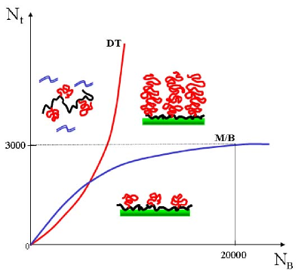
Figure 5: Phase diagram for a comb–polymer with an adsorbing backbone made of $p$ blocks of $N_{B}$ monomers each and non–adsorbing side–chains of $N_{t}$ monomers each. The dashed curve represents the mushroom to brush configuration threshold (M/B) while the solid curve represents the desorption threshold (DT).

where $Z_{t}^{f}(z_{\omega},n|z_{\alpha})$ is the partition function of an non–adsorbed strand of $n$ monomers starting at $z_{\alpha}$ and ending at $z_{\omega}$, $Z^{f}_{t}(z_{\omega},n)$ is obtained after integration of $Z_{t}^{f}(z_{\omega},n|z_{\alpha})$ over $z_{\alpha}$. These partition functions are discussed in Appendix C. The expressions (19) for the loops and tails contributions to the total monomer volume fraction for a triblock copolymer of $N\sim N_{B}$ monomers are the same as the one found for the adsorption of a linear polymer chain of $N_{B}$ monomers. For the side–chains monomer volume fraction $\Phi^{\rm TB}_{\rm sc}(z)$, one finds (see Fig.5):

$$\Phi^{\rm TB}_{\rm sc}(z)\quad=\quad\left\{\begin{array}[]{lll}\displaystyle{\frac{\Gamma_{o}}{N_{B}\,R_{t}}}&\quad z^{2}&\quad d<z<R_{t},\\ \displaystyle{\frac{\Gamma_{o}\,R_{t}^{3}}{N_{B}}}&\quad z^{-2}&\quad R_{t}<z<z^{*},\\ \Gamma_{o}\,R_{t}^{3}\,N_{B}&\quad z^{-8}&\quad z^{*}<z<\lambda,\end{array}\right.$$ (20)

where $\lambda$ is the average thickness of the triblock copolymer adsorbed layer. Close to the wall, $d<z<R_{t}$, where the side chains are depleted, the side–chain volume fraction is constructed from chemically close junction points, each of which contributes $z^{2}$ monomers (one blob). Further from the wall, the side–chain density follows the junction point density (with the normalization factor $N_{t}$). At short distances, in the adsorbed loops layer, $\Phi_{\ell}(z)$ dominates over the other contributions, at large distances, $\Phi(z)\sim\Phi_{t}(z)$. As for linear chain adsorption, the characteristic length $z^{*}$ represents the length–scale inside the adsorbed layer (where the adsorption energy $\epsilon$ is negligible compared to the effective potential $U(z)$), at the cross–over from the loops–dominated layer to the tails dominated layer:

$$\begin{array}[]{lll}z^{*}&\sim&\left[N\,b\;\ln{\left(\displaystyle{\frac{N_{B}}{b^{2}}}\right)}\right]^{1/3}\;\sim\;(N_{B}\,b)^{1/3},\end{array}$$ (21)

which is the same as the one found for the adsorption of a linear chain of $N_{B}$ monomers.

The thickness of the adsorbed triblock copolymer layer $\lambda\sim\epsilon^{-1/2}$ is smaller than the thickness of a linear polymer adsorbed layer:

$$\lambda\quad=\quad\lambda_{o}\left[1\,+\,\lambda_{o}^{2}\,\displaystyle{\frac{\ln{(\Gamma_{o}\,R_{t})}}{N_{B}}}\right]^{-1/2},$$ (22)

where

$$\lambda_{o}\quad=\quad\left(\frac{N_{B}\,a^{2}}{6}\right)^{1/2}\,\ln{\left(\frac{1}{\Phi_{b}\,b^{2}}\right)}^{-1/2}.$$ (23)

If $N_{t}$ increases, $\lambda$ decreases, as the adsorption is partially prevented by the presence of the side–chains.
From the complete expression for the triblock copolymer volume fraction $\Phi(z)$ (see Eq.(18),(19) and (20)), one can calculate the correction to the surface coverage (of backbone monomers) due to the side–chains:

$$\Gamma\quad=\quad\Gamma_{o}\;\left[1-\frac{2}{\Gamma_{o}\,\lambda}\;+\;\frac{N_{t}}{N_{B}}\,\left(2\,-\,\frac{R_{t}}{z^{*}}\right)\right].$$ (24)

II.4.1 From Triblock Copolymers to Combs

Once the adsorption profiles in triblock copolymer adsorbed layers are known, it is straightforward to extend the study to comb–like architectures. The combs are linear polymers made of $p$ sub–units ($p\geq 1$), which are triblock copolymers with an adsorbing backbone of $N_{B}$ monomers and size $R_{B}=N^{1/2}a$ and one non–adsorbing side–chain of $N_{t}$ monomers, with $N_{t}\ll N_{B}$. The total number of monomers per comb is $N\,=\,p\,(N_{B}+N_{t})\sim p\,N_{B}$.
Far from the adsorbing surface, i.e. for $z\gg R_{B}$, the comb–polymer can be seen as a chain of blobs, each being a triblock copolymer. The density of cores (branching points) and the volume fraction of side chain monomers are therefore $\rho_{c}(z)=2\,z^{-2}/N_{B}$ and $\Phi_{\rm sc}(z)=2\,N_{t}\,z^{-2}/N_{B}$. Close to the surface, Eq.(20) for triblock copolymer adsorption correctly predicts the structure of the comb side–chains adsorption profile $\Phi_{\rm sc}(z)={\frac{\Gamma_{o}\,R_{t}^{3}}{N_{B}}}z^{-2}$. These two predictions crossover smoothly. There is therefore an intermediate regime involving a new length scale. There is actually a strong constraint that loops smaller than $N_{B}$ monomers cannot contain more than one branching point. The profile given by Eq.(20) is thus valid only up to a distance $z_{1}$ where each loop comprises a number of side–chains of order one. One can estimate the fraction $x$ of loops of size $z$ that contain one side–chain, $x=\rho_{c}/\rho_{l}$, where the loops density $\rho_{l}$ is given by the monomer density divided by the number of monomers per loop $g(z)\sim z^{2}$ (Gaussian loops), $\rho_{l}(z)\sim z^{-4}$. This fraction is smaller than one if $z<z_{1}$, where

$$z_{1}\quad=\quad\left(\displaystyle{\frac{N_{B}}{N_{t}^{1/2}}}\right)^{1/2},$$ (25)

At distances $z_{1}<z<R_{B}$, all loops contain a branching point and $x\sim 1$, i.e. $\rho_{c}(z)\sim\rho_{l}(z)$. This description holds as long as the adsorbed combs are in a mushroom regime, i.e. for $R_{t}<z_{1}<R_{B}$, which leads to the same threshold derived at the end of Section II.3 for the crossover from a mushroom to a brush configuration for the adsorbed triblock copolymers:

$$N_{t}<N_{B}^{2/3}.$$ (26)

The structure of the adsorbed layer is mainly determined by the small loop structure close to the wall which is the same for comb and triblock copolymers. In particular, the monomer chemical potential $\epsilon$ is the same in both cases. This gives the adsorbed layer thickness of a comb–polymers comprising $p$ blocks, $\lambda_{p}=\sqrt{p}\lambda$ where $\lambda$ is given by Eq.(22). In Table 1 we present a summary of the mean field behavior of the comb–polymers branching point density and monomer volume fraction in the adsorbed layer.

	$0\leq z\leq R_{t}$	$R_{t}\leq z\leq z_{1}$	$z_{1}\leq z\leq R_{B}$	$R_{B}\leq z\leq\lambda_{p}$
$\rho_{c}(z)$	$\frac{\Gamma_{o}}{N_{B}\,R_{t}}$	$\frac{\Gamma_{o}\,R_{t}}{N_{B}}\;z^{-2}$	$\Gamma_{o}\,z^{-4}$	$\frac{\Gamma_{o}}{N_{B}}\;z^{-2}$
$\Phi^{\rm co}_{\rm sc}(z)$	$\frac{\Gamma_{o}}{N_{B}\,R_{t}}\;z^{2}$	$\frac{\Gamma_{o}\,R_{t}^{3}}{N_{B}}\;z^{-2}$	$\Gamma_{o}\,N_{t}\;z^{-4}$	$\frac{\Gamma_{o}\,N_{t}}{N_{B}}\;z^{-2}$

Table 1: Mean field branching point density $\rho_{c}(z)$ and monomer volume fraction $\Phi_{\rm sc}(z)$ for an adsorbed comb–polymer (z is the vertical coordinate above the adsorbing surface).

III Comb–Copolymer Adsorption: Scaling Approach

III.1 Comb–Copolymer Mushroom Regime: Scaling

We now generalize our description of the adsorption of a comb–polymer in a mushroom configuration ($R_{t}<z_{1}$) using a scaling approach. As in the mean field theory, the side–chains give only a very small perturbation to the concentration profile and the total monomer concentration profile decays with the same power law as that of adsorbed linear polymer chains $\Phi(z)\sim z^{1/\nu-d}$, where $\nu\approx 0.59$ is the Flory scaling exponent and $d=3$ the space dimension de Gennes (1980). For each of the regimes found in the mean field theory, we now derive the corresponding scaling laws.

At distances from the adsorbing surface larger than the Flory radius of the side chains $R_{t}\sim a\,N_{t}^{\nu}$, the side–chains behave essentially as free chains. As in the mean field theory, if $R_{t}<z<z_{1}$, the density of side–chains is proportional to the total monomer density and $\Phi_{\rm sc}(z)=c_{1}\cdot z^{1/\nu-d}$. The constant $c_{1}$ is determined by imposing the conservation of the side–chain monomers, $\int\Phi_{\rm sc}(z)\,{\rm d}z=\Gamma\,N_{t}/N_{B}$, leading to:

$$\Phi_{\rm sc}(z)\quad = \quad\displaystyle{\frac{\Gamma\,N_{t}}{N_{B}\,R_{t}}}\cdot\left(\displaystyle{\frac{R_{t}}{z}}\right)^{d-\frac{1}{\nu}},\qquad R_{t}<z<z_{1}$$

$$\rho_{c}(z)\quad = \quad\Phi_{\rm sc}(z)/N_{t}.$$ (27)

At larger distances $z_{1}<z<R_{B}$, each loop carries one side–chain and thus $\rho_{c}(z)=z^{-d}$, $\Phi_{\rm sc}(z)=N_{t}\,z^{-d}$. The crossover between these two regimes occurs at a distance $z_{1}$ given by:

$$z_{1}\quad=\quad a\;\left[\displaystyle{\frac{N_{B}}{N_{t}^{\nu(d-1)-1}}}\right]^{\nu}.$$ (28)

For $d=4$ and $\nu=1/2$, Eq.(28) gives back the mean field result of Section II.4, $z_{1}^{2}=N_{B}/N_{t}^{1/2}$.

Far from the surface, for $z>R_{B}\sim a\,N_{B}^{\nu}$, the comb–copolymer behaves as an effective linear chain of blobs, the individual blobs being triblock copolymers with one side–chain per blob and thus $\rho_{c}(z)=z^{-d+1/\nu}/N_{B}$, $\Phi_{\rm sc}(z)=N_{t}\,z^{-d+1/\nu}/N_{B}$.

At short distances, $0<z<R_{t}$, the density of side chain monomers is dominated by those side–chains for which the junction point belongs to the same blob of size $z$. The density of side–chain monomers is thus equal to the product of the junction point density $\rho_{c}$ by the number of monomers of the side chain in this same blob $z^{1/\nu}$, $\Phi_{\rm sc}(z)\sim z^{1/\nu}\rho_{c}(z)$. To place a branching point at position $z$ we need to place the relevant core monomer and to let a tail of size $N_{t}$ start there. In contrast to the mean field description, the side–chain is correlated with the backbone. The branching point density $\rho_{c}(z)$ is derived in the Appendix D. It is constructed from the backbone monomer density, the partition function of a free tail Semenov and Joanny (1995) and the three leg vertex at the branching point. We obtain:

$$\rho_{c}(z)={\Gamma\over N_{B}R_{t}}\left({z\over R_{t}}\right)^{\alpha}$$ (29)

with an exponent $\alpha=-d/2-1+\gamma/(2\nu)+1/\nu-\theta_{1}\simeq-0.27$. The junction points are thus weakly localized at the surface where excluded volume correlations are screened. The des Cloizeaux exponent $\theta_{1}=(\sigma_{1}-\sigma_{3})/\nu$ is introduced by the three leg vertex (see Appendix D). The side–chain monomer concentration can be deduced as:

$$\Phi_{\rm sc}(z)\quad=\quad z^{1/\nu}\rho_{c}(z)={\Gamma N_{t}\over N_{B}R_{t}}\left({z\over R_{t}}\right)^{\beta},$$ (30)

where the exponent $\beta$ is close to $1.4$.

Summarizing, for $R_{t}<z_{1}$, i.e. in the mushroom regime for the comb–polymer, the side–chains monomer volume fraction is given by:

$$\Phi_{\rm sc}(z)\quad=\quad\left\{\begin{array}[]{ll}\displaystyle{\frac{\Gamma\,N_{t}}{N_{B}\,R_{t}}}\cdot\left(\displaystyle{\frac{z}{R_{t}}}\right)^{-d/2-1+\gamma/(2\nu)+2/\nu-\theta_{1}}&0\leq z\leq R_{t},\\ \displaystyle{\frac{\Gamma\,N_{t}}{N_{B}\,R_{t}}}\cdot\left(\displaystyle{\frac{R_{t}}{z}}\right)^{d-\frac{1}{\nu}}&R_{t}\leq z\leq z_{1},\\ \displaystyle{\frac{N_{t}}{z^{d}}}&z_{1}\leq z\leq R_{B},\\ \displaystyle{\frac{N_{t}}{N_{B}}}\;z^{\frac{1}{\nu}-d}&R_{B}\leq z\leq\lambda_{p}.\end{array}\right.$$ (31)

III.2 Comb–Copolymer Brush Regime: Scaling

So far, we have only considered the mushroom limit where the side–chains do not interact. The number of side chains per unit area in the proximal layer of thickness $R_{t}$ is $\sigma=\Gamma/N_{B}$ and the side chains interact if $\sigma R_{t}^{d-1}>1$; in this case the side chains stretch and form a polymer brush. This occurs if $R_{t}\geq z_{1}$ or as we have shown in Section II.4.1, the adsorbed combs enter the brush regime for:

$$N_{t}\geq N_{B}^{\frac{1}{\nu\,(d-1)}}.$$ (32)

In the mean field approximation, ($d=4$ and $\nu=1/2$) this condition gives $R_{t}\sim N_{B}^{1/3}\sim z^{*}$, in agreement with our mean field results of Section II.3 for the cross–over from the mushroom to brush configuration. We will limit our analysis to the study of strong backbone adsorption and thus we assume that the occurrence of large backbone loops with many side–chains anchored is negligible.

In the brush regime, the side–chains extend into the bulk from their anchoring point on the backbone in a sequence of blobs of size $D_{b}\sim a\,g^{\nu}$, where $g\sim\sigma^{-1/\nu(d-1)}$ is the number of monomers per blob. The grafting density is $\sigma=\Gamma/N_{B}$ and the blob size is $D_{b}\sim a\,N_{B}^{1/(d-1)}$. The concentration of side–chain monomers belonging to the first blob close to the surface is the same as the concentration in an adsorbed layer of comb–copolymers where the side chains would have $g$ monomers or a radius $D_{b}$. It is obtained from the results of the previous section by replacing $N_{t}$ by $g$ and $R_{t}$ by $D_{b}$. The cross–over length $z_{1}$ is then given by $z_{1}=a\,N_{B}^{1/(d-1)}=D_{b}$ and the density of side–chain monomers in the brush

$$\Phi_{\rm sc}(z)\quad=\quad\displaystyle{\frac{\Gamma}{N_{B}\,z_{1}^{1-\frac{1}{\nu}}}}\cdot\left(\displaystyle{\frac{z}{z_{1}}}\right)^{\frac{\gamma}{2\,\nu}+\frac{(d-2)}{2}}.$$ (33)

The thickness of the brush in the blob model is

$$L\;\sim\;a\,N_{t}\;\sigma^{\frac{1-\nu}{\nu\,(d-1)}}\sim a\,N_{t}\,N_{B}^{-\frac{1-\nu}{\nu\,(d-1)}}.$$ (34)

The free energy of the side chains is $k_{b}\,T$ per blob or per side chain

$$\;F_{t}\,\sim\,\left(\frac{a^{2}}{k_{b}\,T}\right)N_{t}\cdot\sigma^{1/\nu(d-1)}\sim\,\left(\frac{a^{2}}{k_{b}\,T}\right)N_{t}\cdot N_{B}^{-1/\nu(d-1)}$$ (35)

The adsorption energy of the backbone chains must compensate the stretching energy of the side–chain brush. This requires an adsorption energy per monomer $\epsilon\sim F_{t}/N_{B}\sim N_{t}\cdot N_{B}^{-(1+1/\nu(d-1))}$. The thickness of the adsorbed backbone layer is then $\lambda_{c}\sim a/\epsilon^{\nu}$ or

$$\lambda_{c}\quad\sim\quad a\;\displaystyle{\frac{N_{B}^{\nu+\frac{1}{d-1}}}{N_{t}^{\nu}}},$$ (36)

As the length of the side chains increases and becomes larger than $N_{t}\ll N_{B}^{1/(d-1)\,\nu}$, the thickness of the backbone adsorbed layer decreases from the radius $R_{B}$ between two branching points and the adsorbed polymer amount decreases. The adsorbed layer is only stable if its thickness is larger than the proximal distance $b$ introduced in Eq.(1). For longer side chains, there is no adsorption of the comb–copolymer

$$N_{t}\geq N_{B}^{1+\frac{1}{\nu(d-1)}},$$ (37)

where the exponent $1+1/\nu(d-1)$ is equal to $11/6$ for swollen chains ($d=3$ and $\nu=3/5$) in a good solvent.

IV Conclusions

We propose here a theoretical investigation of the adsorption of partly adsorbing comb–copolymers, with an adsorbing skeleton and non–adsorbing side–grafts. Three regimes were identified: a ”mushroom” regime characterized by having an adsorbed backbone layer on the surface and the side–chains dangling from the backbone in a swollen state, a ”brush” regime in which they develop a uniform multi–chains coating with an extended layer of non–adsorbing segments, and a non–adsorbed regime. Depending on the size of side–chains, size of skeleton length between side–chains, and adsorption parameters, the scaling laws for the transitions between the different regimes, the adsorption free energy and the thickness of adsorbed layers are derived using a combination of mean field and scaling approaches. In the case of swollen (ideal) chains, $\nu=3/5$ and $d=3$ ($\nu=1/2$ and $d=4$), the threshold between mushroom and brush configurations and the desorption threshold can be expressed as $N_{t}>N_{B}^{5/6}$ ($N_{t}>N_{B}^{2/3}$) and $N_{t}\sim N_{B}^{11/6}$ ($N_{t}\sim N_{B}^{5/3}$). In the brush regime we find that the thickness of the backbone adsorbed layer and the vertical extension of the brush for a swollen (ideal) chain scale as $\lambda_{c}\sim a\,N_{B}^{11/10}\,N_{t}^{-3/5}$ ($\lambda_{c}\sim a\,N_{B}^{5/6}\,N_{t}^{-1/2}$) and $L\sim a\,N_{t}\,N_{B}^{-1/3}$ ($L\sim a\,N_{t}\,N_{B}^{-1/3}$), respectively. These predictions could be checked quantitatively, by experiments able to investigate polymer adsorption, such as Neutron or X–ray reflectometry, ellipsometry, quartz microbalance, or Surface Force Apparatus, and work is currently in progress in our group in this direction. Qualitatively, this new family of copolymers can lead to rather thick layers, without the difficulty often encountered when trying to prepare long conventional (i.e. diblock or triblock) copolymers. These multiblock copolymers may thus be interesting in numerous applications, in which the adsorption of rather large objects (proteins, cells) should be prevented, or controlled. They already demonstrated very interesting performances in the context of DNA sequencing and capillary electrophoresis. In this application, the interesting regime is probably the ”brush” regime, because a uniform layer with no access of the analytes to the wall is wanted. The extension of the brush leads to thicker layers, which should be favorable, but also smaller adsorption free energies, so that a compromise has to be found. Probably, a ”weakly extended” brush is a good aim on the practical side. An important aspect of the problem, on the practical side, is the adsorption kinetics. It has been well recognized that the adsorption of large polymers on surfaces is strongly constrained by the kinetics of penetration of a new polymers across the already adsorbed layer, so that the thermodynamic equilibrium, which is discussed in the present article, can be hard to reach. The adsorption kinetics of high molecular weight polymers is a very difficult problem on the theoretical side, and it is beyond the scope of the present article. We believe, however, that numerous information useful for experimental development of applications can be gained from the present approach. In particular, there are practical ways to minimize kinetic barriers to adsorption, e.g. by performing adsorption from a semi–dilute, rather than dilute, solution.

Acknowledgments: A.S. acknowledges a ”Marie Curie” Postdoctoral fellowship from the EU (HPMF-CT-2000-00940) and thanks Dr. P. Sens for very valuable discussions. This work was partly supported by a grant from Association pour la Recherche sur le Cancer (ARC).

Appendix

IV.1 Triblock copolymer: Monomer Volume Fraction

$$\begin{array}[]{lll}\Phi_{\rm\ell}(z)\quad=\quad\left\{\begin{array}[]{lll}2&(z+d)^{-2}&\quad 0\leq z\leq z^{*},\\ z^{*^{6}}&z^{-8}&\quad z^{*}\leq z\leq\lambda,\end{array}\right.\\ \\ \Phi_{\rm t}(z)\quad=\quad\left\{\begin{array}[]{ll}\displaystyle{\frac{z}{N_{B}}}\,\ln\left[\frac{z^{*}}{z}\right]&0<z<z^{*},\\ z^{-2}&z^{*}<z<\lambda,\end{array}\right.\\ \\ \Phi^{\rm TB}_{\rm sc}(z)\quad=\quad\left\{\begin{array}[]{lll}\displaystyle{\frac{\Gamma_{o}}{N_{B}\,R_{t}}}&\quad z^{2}&\quad d<z<R_{t},\\ \displaystyle{\frac{\Gamma_{o}\,R_{t}^{3}}{N_{B}}}&\quad z^{-2}&\quad R_{t}<z<z^{*},\\ \Gamma_{o}\,R_{t}^{3}\,N_{B}&\quad z^{-8}&\quad z^{*}<z<\lambda,\end{array}\right.\end{array}$$ (38)

where $z^{*}=(N\,b\,\log({N/b^{2}}))^{1/3}$.

$$\Phi^{\rm TB}(z)\;=\;\left\{\begin{array}[]{ll}2\;(z+d)^{-2}\,+\,\frac{\Gamma_{o}}{N_{B}\,R_{t}}\cdot z^{4}\,+\,\displaystyle{\frac{z}{N_{B}}}\;\ln\left(\displaystyle{\frac{z^{*}}{z}}\right)&\quad 0\leq z\leq R_{t},\\ \\ \left[2\,+\,\displaystyle{\frac{\Gamma_{o}\,R_{t}^{3}}{N_{B}}}\right]\;z^{-2}\;+\;\displaystyle{\frac{z}{N_{B}}}\;\ln\left(\displaystyle{\frac{z^{*}}{z}}\right)&\quad R_{t}\leq z\leq z^{*},\\ \\ z^{-2}\;+\;\left[z^{*^{6}}\;+\;\Gamma_{o}\,R_{t}^{3}\,N_{B}\right]\cdot z^{-8}&\quad z^{*}\leq z\leq\lambda\end{array}\right.$$ (39)

IV.2 Comb–Copolymer: Side–Chains Monomer Volume Fraction

$$\Phi^{\rm co}_{\rm sc}(z)\quad=\quad\left\{\begin{array}[]{lll}\displaystyle{\frac{\Gamma_{o}}{N_{B}\,R_{t}}}\;z^{2}&0<z<R_{t}\\ \displaystyle{\frac{\Gamma_{o}\,R_{t}^{3}}{N_{B}}\;z^{-2}}&R_{t}<z<z_{1}\\ \Gamma_{o}\,N_{t}\;z^{-4}&z_{1}<z<R_{B}\\ \Gamma_{o}\,\displaystyle{\frac{N_{t}}{N_{B}}}\;z^{-2}&R_{B}<z<\lambda_{p}\end{array}\right.$$ (40)

IV.3 Propagator and Partition Function of a Side–chain in a Triblock Copolymer Adsorbed Layer

IV.3.1 Chain Propagator

We calculate here the propagator of a side chain in the triblock copolymer adsorbed layer between the junction point at coordinate $z_{c}$ and and the free end point at coordinate $z$, $Z_{t}^{f}(z,N_{t}|z_{c})$. The Laplace transform of this propagator $\tilde{Z}_{t}^{f}(z,p|z_{c})=\int_{0}^{\infty}dN_{t}\exp-(p\,N_{t})\;Z_{t}^{f}(z,N_{t}|z_{c})$

$$-\delta(z-z_{c})\quad=\quad{\partial^{2}\tilde{Z}_{t}^{f}(z,p|z_{c})\over\partial z^{2}}\,-\,(p+{2\over z^{2}})\;\tilde{Z}_{t}^{f}(z,p|z_{c}),$$ (41)

with the boundary condition that it vanishes at the wall $z=0$. The solution of this equation is

$$\tilde{Z}_{t}^{f}(z,p|z_{c})\quad=\quad f_{-}(z_{<})\;f_{+}(z_{>}),$$ (42)

where we have defined $z_{<,>}=\mbox{ min,max}(z_{c},z)$. The functions $f_{+}$ and $f_{-}$ are given by

$$f_{+}(z,p) = \sqrt{\pi\over 2p}\;e^{-\sqrt{p}z}\;\left(1+{1\over z\sqrt{p}}\right),$$

$$f_{-}(z,p) = \sqrt{2\over\pi}\;\left(\cosh(\sqrt{p}z)-{\sinh(\sqrt{p}z)\over\sqrt{p}z}\right).$$ (43)

The following asymptotic limits are useful:

$$z_{>} \ll R_{t}\quad\tilde{Z}_{t}^{f}(z,p=0|z_{c})={z_{<}^{2}\over 3z_{>}},$$ (44)

$$z_{<} \gg R_{t}\quad\tilde{Z}_{t}^{f}(z,p|z_{c})={1\over 2\sqrt{p}}e^{-\sqrt{p}(z_{>}-z_{<})}\;\lim_{p\rightarrow\infty}{1\over p}\;\delta(z-z_{c}).$$ (45)

IV.3.2 Partition Function

The partition function of a side–chain $Z_{t}^{f}(z_{c})$ with the junction point at position $z_{c}$ is obtained by integration of $\tilde{Z}_{t}^{f}(z,p|z_{c})$:

$$\tilde{Z}_{t}^{f}(z_{c},p)=f_{-}(z_{c},p)\int_{z_{c}}^{\infty}f_{+}(z,p)\;{\rm d}z+f_{+}(z_{c},p)\int_{0}^{z_{c}}f_{-}(z,p)\;{\rm d}z.$$ (46)

At short distances from the wall $z_{c}\ll R_{t}$, the partition function is dominated by the contribution to the integral coming from $z>z_{c}$:

$$\tilde{Z}_{t}^{f}(z_{c},p) = -{z_{c}^{2}\over 3}\log(\sqrt{p}z_{c}),$$ (47)

$$Z_{t}^{f}(z_{c},N_{t}) = {z_{c}^{2}\over 6N_{t}}.$$ (48)

At larger distances from the wall, $z_{c}\gg R_{t}$ the two integrals are equal to $1/2p$ and $Z(z_{c},N_{t})=1$; the side chains are almost free chains.

The density of copolymer junction points $\rho_{c}^{\rm TB}(z)$ and the side–chain monomers volume fraction $\Phi_{sc}^{\rm TB}$ can be calculated using these more precise values of the propagator and partition function; one finds the following results:

$$\begin{array}[]{lll}\rho_{c}^{\rm TB}(z)\quad=\quad\left\{\begin{array}[]{ll}\displaystyle{{1\over N_{B}\,R_{t}}}&\quad z\ll R_{t},\\ \\ \displaystyle{{1\over N_{B}}{R_{t}\over z^{2}}}&\quad R_{t}\ll z\ll z^{\star},\end{array}\right.\\ \\ \Phi_{sc}^{\rm TB}(z)\quad=\quad\left\{\begin{array}[]{ll}\rho^{\rm TB}_{c}(z<R_{t})\cdot z^{2}&\quad z\ll R_{t},\\ \rho^{\rm TB}_{c}(z)\cdot N_{t}&\quad z\gg R_{t}.\end{array}\right.\end{array}$$

These results are similar to those obtained in the main text.

IV.4 Density of Comb–Copolymer Branching Points

In order to determine using scaling arguments the density of branching points of the comb–copolymer at a distance $z_{c}$ smaller than the side chain radius, we first calculate the partition function $Z^{f}_{t}(z_{c},R_{t})$ of a side chain with the branching point at position $z_{c}$ and radius $R_{t}$.

In the limit where $z_{c}$ is of the order of a monomer size $a$, the side–chain behaves as a tail in the adsorbed layer and $Z^{f}_{t}(a,R_{t})\sim R_{t}^{\frac{\gamma-\nu(d-2)}{2\nu}-\frac{1}{\nu}}$.

We now consider the case where $z_{c}=R_{t}$. The probability to find a side chain at a distance $z_{c}$ is proportional to the local monomer concentration $c(z_{c})\sim z_{c}^{1/\nu-d}$. If the side chain is not connected to the backbone but is free, its partition function is $Z^{o}\sim z_{c}^{(\gamma-1)/\nu}$. The partition function of the side chain also contains a factor associated to the branching point. This is best written in terms of the vertex exponents introduced by Duplantier Duplantier (1989). In the partition function of a branched polymer chain, each vertex having $k$ legs is associated, for a chain of size $z_{c}$, to a factor $z_{c}^{\sigma_{k}/\nu}$ where $\sigma_{k}$ is the corresponding vertex exponent. The formation of a branching point in the comb–copolymer corresponds to the disappearance of a two legs vertex on the backbone and a one leg vertex (the side–chain free end) and the appearance of a three legs vertex (the branching point); it is therefore associated to a weight $z_{c}^{(\sigma_{3}-\sigma_{1}-\sigma_{2})/\nu}$. Note that it is sufficient to consider that the backbone chain has a size $z_{c}$ since, in an adsorbed polymer layer, the local screening length is the distance to the adsorbing surface $z_{c}$. Considering all these factors, we obtain the partition function

$$Z^{f}_{t}(z_{c},R_{t})\sim z_{c}^{(1-d\nu+\gamma-1+\sigma_{3}-\sigma_{2}-\sigma_{1})/\nu}\sim z_{c}^{\gamma/\nu-d-\theta_{1}}.$$ (49)

We have here used the fact that $\sigma_{2}=0$ and introduced the contact exponent $\theta_{1}=(\sigma_{1}-\sigma_{3})/\nu\simeq 0.45$ first considered by Des Cloizeaux Cloizeaux and Janink (1987).

The partition function $Z^{f}_{t}(z_{c},R_{t})$ is obtained by a scaling law extrapolating between these two asymptotic limits

$$Z^{f}_{t}(z_{c},R_{t})\sim z_{c}^{\alpha}R_{t}^{\frac{\gamma-\nu(d-2)}{2\nu}-\frac{1}{\nu}},$$ (50)

with an exponent $\alpha=-d/2-1+\gamma/2\nu+1/\nu-\theta_{1}\simeq-0.27$.

The density of branching points is proportional to this partition function; the pre–factor is obtained by imposing that the total number of branching points per unit area over a thickness $R_{t}$ is of order $\Gamma/N_{B}$:

$$\rho_{c}(z_{c})={\Gamma\over N_{B}R_{t}}{\left(z_{c}\over R_{t}\right)}^{\alpha}$$ (51)

$\Phi_{b}$	Bulk monomer volume fraction
$N=p\,(N_{B}\,+\,N_{t})$	Total number of monomers per comb–polymer
$p$	Number of triblock sub–units per comb–polymer
$N_{B}$	Number of backbone monomers per triblock
$N_{t}$	Number of side–chain monomers per triblock
a	Monomer size ($\sim$ nm)
$\epsilon_{o}$	adsorption energy per monomer of a linear chain
$\epsilon$	adsorption energy per monomer of a comb–polymer
b	Extrapolation length ($\sim 1/\epsilon_{o}$ for adsorbing linear chains)
$R_{t}=a\sqrt{N_{t}}$	Side–chain gyration radius
$R_{B}=a\sqrt{N_{B}}$	gyration radius of backbone monomers for a triblock
$z^{*}$	Thickness of loops dominated layer over the adsorbing surface
$\lambda$	Total thickness of the adsorbed layer
$Z^{o}_{N_{B}}(z)$	Partition function of a linear backbone adsorbing chain made of $N_{B}$
	monomers and with one end at position $z$ above the adsorbing surface
$Z_{N}^{f}(z)$	Partition function of a non–adsorbed linear chain of N monomers
$Z_{N}(z)$	Partition function of a triblock made of N monomers and
	with one end at position $z$ above the adsorbing surface
$\Gamma_{o}$	Surface coverage (number of monomers per unit surface) for a
	linear chain
$\Gamma$	Surface coverage (number of monomers per unit surface) for a
	comb–polymer
$L$	Side–chains brush vertical extension
$\sigma$	Surface grafting density
$d$	Space dimension

Table 2: Table of Symbols.

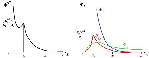
Figure 4: Triblock’s monomer volume fraction $\Phi^{\rm TB}_{\rm sc}=\Phi_{\ell}+\Phi_{t}+\Phi_{\rm sc}$: loops ($\Phi_{\ell}(z)$), tails ($\Phi_{t}(z)$) and side–chains ($\Phi_{\rm sc}(z)$) contributions.

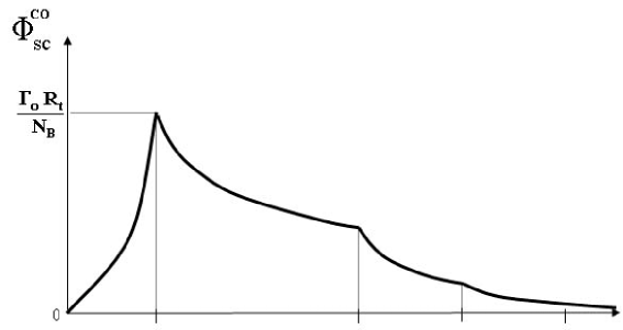
Figure 6: Combs side–chains monomer volume fraction, $\Phi^{\rm co}_{\rm sc}(z)$.

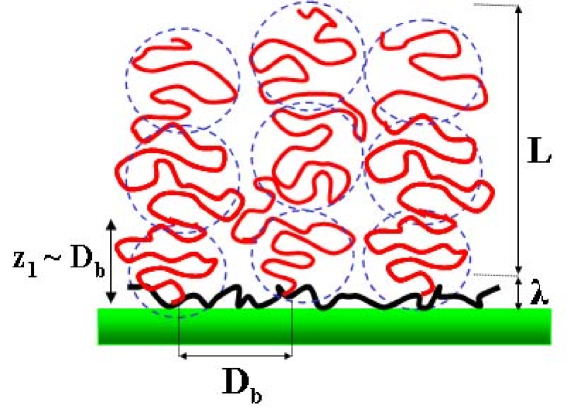
Figure 7: Brush regime for a comb–polymer with an adsorbing backbone made of $p$ blocks of $N_{B}$ monomers each and with $p$ non–adsorbing side–chains of $N_{t}$ monomers each, with $N_{t}\gg N_{B}$.

References

- Hjerten and Kubo (2000) S. Hjerten and K. Kubo, Electrophoresis 14, 390 (2000).
- Marshall and Pennisi (1998) E. Marshall and E. Pennisi, Science 280, 994 (1998).
- Salas-Solano et al. (2000) O. Salas-Solano, D. Schmalzing, L. Koutny, S. Buonocore, A. Adourian, P. Matsudaira, and D. Ehrlich, Anal. Chem. 72, 3129 (2000).
- Carrilho (2000) E. Carrilho, Electrophoresis 21, 55 (2000).
- Viovy (2000) J.-L. Viovy, Rev. Mod. Phys. 72, 813 (2000).
- Ajdari (1995) A. Ajdari, Phys. Rev. Lett. 75, 755 (1995).
- Horvath and Dolnik (2001) J. Horvath and V. Dolnik, Electrophoresis 22, 644 (2001).
- Righetti et al. (2001) P. G. Righetti, C. Gelfi, B. Verzola, and L. Castelletti, Electrophoresis 22, 603 (2001).
- Doherty et al. (2002) E. A. Doherty, K. D. Berglund, B. A. Buchholz, I. V. Kourkine, T. M. Przybycien, R. D. Tilton, and A. E. Barron, Electrophoresis 23, 2766 (2002).
- Liang et al. (2001) D. Liang, T. Liu, L. Song, and B. Chu, J. Chrom. 909, 271 (2001).
- Liang and Chu (1998) D. Liang and B. Chu, Electrophoresis 19, 2447 (1998).
- Madabhushi (1998) R. S. Madabhushi, Electrophoresis 19, 224 (1998).
- Chiari et al. (2000) M. Chiari, M. Cretich, and J. Horvath, Electrophoresis 21, 1521 (2000).
- Albarghouthi et al. (2001) M. N. Albarghouthi, B. A. Buchholz, E. A. Doherty, F. M. Bogdan, H. Zhou, and A. E. Barron, Electrophoresis 22, 737 (2001).
- Zhou et al. (2000) H. Zhou, A. W. Miller, Z. Sosic, B. Buchholz, A. E. Barron, L. Kotler, and B. L. Karger, Anal. Chem. 72, 1045 (2000).
- Barbier et al. (2002) V. Barbier, B. A. Buchholz, A. E. Barron, and J.-L. Viovy, Electrophoresis 23, 1441 (2002).
- Joanny and Johner (1996) J.-F. Joanny and A. Johner, J. Phys. II France 6, 511 (1996).
- Semenov et al. (1996) A. N. Semenov, J. Bonet-Avalos, A. Johner, and J.-F. Joanny, Macromolecules 29, 2179 (1996).
- Semenov et al. (1998) A. N. Semenov, J.-F. Joanny, and A. Johner, in Theoretical and Mathematical Models in Polymer Research (Academic Press, 1998), pp. 37–82.
- Marques and Joanny (1989) C. M. Marques and J.-F. Joanny, Macromolecules 22, 1454 (1989).
- Johner and Joanny (1997) A. Johner and J.-F. Joanny, Macromol. Theory Simul. 6, 479 (1997).
- Gennes (1981) P. G. D. Gennes, Macromolecules 14, 1637 (1981).
- de Gennes (1980) P. G. de Gennes, Macromolecules 13, 1069 (1980).
- Marques and Joanny (1990) C. M. Marques and J.-F. Joanny, Macromolecules 23, 268 (1990).
- Marques et al. (1988) C. M. Marques, J.-F. Joanny, and L. Leibler, Macromolecules 21, 1051 (1988).
- Grosberg and Khoklov (1994) A. Y. Grosberg and A. R. Khoklov, Statistical Physics of Macromolecules (AIP Press, New York, 1994).
- Semenov and Joanny (1995) A. N. Semenov and J. F. Joanny, Europhys. Lett. 29, 279 (1995).
- Duplantier (1989) B. Duplantier, J.Stat.Phys. 54, 581 (1989).
- Cloizeaux and Janink (1987) J. D. Cloizeaux and G. Janink, Les Polymères en Solution: leur modélisation et leur structure (Editions de Physique, 1987).