Application of a two–length scale field theory to the solvation of charged molecules: I. Hydrophobic effect revisited

Abstract

On a basis of a two–length scale description of hydrophobic interactions we develop a continuous self–consistent theory of solute–water interactions which allows to determine a hydrophobic layer of a solute molecules of any geometry with explicit account of solvent structure described by its correlation function. We compute the mean solvent density profile $n(r)$ surrounding the spherical solute molecule as well as its solvation free energy $\Delta G(r)$. We compare the two–length scale theory to the numerical data of Monte–Carlo simulations found in the literature and discuss the possibility of a self–consistent adjustment of the free parameters of the theory. In the frameworks of the discussed approach we compute also the solvation free energies of alkane molecules and the free energy of interaction $\Delta G(D)$ of two spheres of radius $R$ separated by the distance $D$. We describe the general setting of the self–consistent account of electrostatic interactions in the frameworks of the model where the water is considered not as a continuous media, but as a gas of dipoles. We analyze the limiting cases where the proposed theory coincides with the electrostatics of a continuous media.

I Introduction

We consider the current work as a step towards the development of a continuous thermodynamic theory of solute–solvent interactions. The construction of such a kind of a theory is of extreme importance for biochemical applications connected with the reliable and fast determination of the protein–ligand binding constants in solvent (water) with the precision comparable to the accuracy of explicit molecular–dynamical simulations.

There are few kinds of approaches which take into account the effect of fluctuating media on interactions between solvated molecules. Tentatively we can split them into the following three groups:

i) ”Explicit approaches”. Generally such methods are based on numerical simulations taking into account motion of many water molecules. Such approaches are very time consuming because they demand huge computational resources.

ii) ”Implicit approaches”. These: a) either exploit the heuristic concepts of the ”surface area accessible by the solvent” and of the ”width of the hydrophobic layer”, or b) make some effective renormalization of ”bare” (i.e. vacuum) parameters of interacting molecules: in the frameworks of these approaches the effect of water on thermodynamic properties of dissolved substances is computed on the basis of some additional data on solubility, evaporation etc—see, for example, george ; gav ; finkelstein .

iii) ”Intermediate approaches”. The works belonging to that group (including our one), offer attempts which, on one hand, get rid of explicit numerical simulation of water molecules, and, on the other hand, preserve an effective account for water. The development of these methods on the basis of a clear understanding of a physical origin of solute–water interactions could, at least, give a better control for the parameters used in implicit approaches.

Most commonly, in the ”implicit approaches” it is assumed surf ; priv that the free energy of solvation is proportional to the solvent accessible surface area of a solute molecule. It is obviously true for solutes much larger than a water molecule. However, for the solutes of sizes comparable to the size of water molecules, as well as for the solutes of complex geometry, the question of the determination of the corresponding hydrophobic layer, being of great importance, is often resolved by means of purely empiric conjectures. For example, it is supposed usually that the hydrophobic layer is equal to the surface covered by a center of a water molecule ”rolling” around the solute surface. Some modifications of the method deal with the so-called ”molecular surface area” – see, for example, msa . Another method of implicit account for the solvent in the so-called ”Gaussian approximation” has been proposed by karp .

Among the theoretical attempts to develop a constructive theory of solvent–solute interactions, the following groups of works (to our point of view) deserve special attention:

1. The detailed computation of the solvent density–density correlation function in the presence of dissolved substances (with or without electrostatics): a) either introducing weighted densities and explicitly designing the form of the density functional which is entirely dictated by physical constraints rosen , or b) by the construction of an appropriate ”bridge functional” (i.e. closure relation) for the correlation function satisfying the hierarchy of integral equations 3drism . On the basis of the correlation function all the thermodynamic quantities can be easily determined.

2. The computation of the averaged profile of the solvent density described by the fluctuating field in presence of solute molecules (with or without electrostatic interactions). The solvent structure on small scales is taken into account by its bulk correlation function, while the effect of solute solvation is considered by forcing the total solvent density to be zero inside the solute molecule (see, for example, chand4 and references therein). Minimization of the corresponding free energy allows one to compute the density and the solvation free energy.

3. The ”Scaled Particle Theory”(SPT) spt ; spt1 and the ”Information Theory” (IT), developed in the series of papers pratt . Both these approaches, SPT and IT, exploit the relation between the probability to find a cavity of a given shape containing some number of particles, with the solvation free energy of a solute molecule of that shape. The probability of a cavity formation in an ensemble of fluctuating particles (water molecules) is computed on the basis of semi–empirical combinatorial arguments.

Our solvation model borrows its ideas in the second group from the list above, namely from the series of works chand1 ; chand2 ; chand3 where a two–length scale description of hydrophobic interactions was developed. In this approach the solvent density is decomposed in two components, the slowly varying field describing the mean solvent (water) density, and the short–ranged density fluctuations. We believe that such an approach is optimal from different points of view: on one hand it is physically clear, being ”semi-microscopic”, and on other hand it can be used as a constructive computational tool of account for water, much faster than the corresponding explicit approaches but without the loss of the precision. So, our aim is to construct a theory of solute–water interactions which would allow to determine the hydrophobic layer of solute molecules of any geometry with account of water structure described by its correlation function. The parameters of such a theory will be determined by testing them for solutes with simple geometries and comparing these cases with the experimental data. Briefly, the main ingredients of our work are as follows:

i) We consider water as a continuous inhomogeneous media and describe it by a fluctuating continuous density field; the discreteness of the water structure on small scales is taken into account through the fluctuations controlled by the water correlation function $\chi$ in the bulk;

ii) The solvation free energy of the substance situated in water is obtained in the self–consistent mean–field approximation based on slightly modified Ginzburg–Landau–Chandler functional chand1 ; chand2 .

Our work is devoted to the calculation of the solvation free energy and of the free energy of interactions of solute molecules of any arbitrary shapes.

Specifically, we start with a two–scale Ginzburg–Landau Hamiltonian and perform an analytical integration over the short–ranged fluctuations. This provides a single–variable Hamiltonian yielding an integro–differential equation. The solution of this equation ensures the equilibrium mean density profile of the water, and the corresponding value of the Hamiltonian gives the solvation free energy. We pay a special attention to the physical clarity and consistency of all steps of derivation of our model. We discuss the hidden dangers on the way and compare our approach to the Monte–Carlo numerical simulations carried out in chand4 . We determine in a self–consistent way the width and the geometry of a hydrophobic layer surrounding the solute molecules. So, we believe that a very important auxiliary goal of our work concerns the prediction of the relevant number of water shells (the ”solvent accessible surface area”) around a solute molecule.

Summarizing the said above, the advantages of the fluctuational approach with respect to other phenomenological theories of ”implicit water” are as follows:

a) There is no difference in computations of the solvation free energy and of the free energy of interactions of solute molecules;

b) The detailed structure of the solvent is taken into account on small scales;

c) We do not need any special determination of the ”hydrophobic layer” by ”rolling” the water molecule around the solute surface. The width and the geometry of a hydrophobic layer is computed on the basis of: a) the true geometry of a solute molecule, and b) the supposition about the solute–selvent and solvent–solvent interactions.

d) The theory contains small number of adjustable parameters, which in turn can be determined from the independent experiments (either numerical, or real).

Our paper is organized as follows. In the Section II we describe the model and derive the basic equations for the equilibrium and the full densities, and for the solvation free energy, as well as we solve numerically the obtained equations, compare them to the numerical Monte–Carlo simulations of the work chand4 and propose the way of tuning the adjustable parameters of the Hamiltonian; in the Secion III we compute the solvation free energy of alkanes, as well as the free energy of interaction of two spherical solute molecules; the results of the work are summarized in the Section IV, where we also derive the equations for electrostatics in fluctuating dipolar environment.

II The model

In this Section we present the self–consistent description of solvation which takes into account simultaneously: i) the smoothly varying average density field $n{(\bf r})$, and ii) the water structure on small scales described by the density–density correlation function $\chi({\bf r},{\bf r}^{\prime})$.

Following the general scheme of the works chand3 , we describe the solvent by two fields: $n({\bf r})$ – the average density varying on long distances, and $\omega({\bf r})$ – the small-scale fluctuating field controlled by the correlation function of the water $\chi({\bf r},{\bf r}^{\prime})=\left<\omega({\bf r})\omega({\bf r}^{\prime})\right>$ in the bulk. The solvent cannot penetrate into the volume occupied by the solute molecule hence the total solvent density $\rho({\bf r})=n({\bf r})+\omega({\bf r})$ is nullified inside the solute: $\rho({\bf r})=0$ for all ${\bf r}\in v_{\rm in}$, where $v_{\rm in}$ is the volume occupied by the solute molecule. The fact that we force the total solvent density $\rho({\bf r})=n({\bf r})+\omega({\bf r})$ to be zero inside the solute, results in an effective interactions between $n({\bf r})$ and $\omega({\bf r})$. In general, one can permit also the direct coupling between $n({\bf r})$ and $\omega({\bf r})$ everywhere in the solute.

The thermodynamic properties of the solvent (water) in the bulk are obtained using the self–consistent Ginzburg–Landau (GL) free energy functional which describes the liquid–vapor phase transition. The average solvent density $n({\bf r})$ plays the role of an order parameter. The interactions between long– and small–scale fields $n({\bf r})$ and $\omega({\bf r})$ can enforce the ”drying”, shifting the liquid–vapor transition. Minimizing the corresponding free energy functional, we compute the desired density profile and the solvation free energy.

It should be noted that the fully microscopic description of the solute–solvent interactions certainly does not require introducing of any scale separation—everything is described by the single microscopic field $\rho({\bf r})$. However in such a description the interactions between water molecules should also be described on the microscopic level. Such kind of theory has been developed in the works rosen . It seems to us that due to the heavy machinery, the application of such approach to the solvation and interactions of objects of complex architecture in water is yet rather restrictive for practical purposes. So, the nature of two different scales in the approach chosen in our work, is the consequence of the mean–field (GL) description of the water–water interactions.

Before going into details let us point out what is different in our consideration with respect to the original two–length scale theory of Chandler et al. chand1 ; chand2 ; chand3 ; chand4 .

i) We do not divide the space in ”cells” for the large–scale field $n({\bf r})$ (as in chand4 ). We describe the system by two fully continuous densities. The equilibrium density is determined selfconsistently without additional averaging over small–scale fluctuations. We believe that this would result in better description of solvation of objects of rough shape and of the free energy of interactions between solutes located close to each other.

ii) We can tune the potential $W(n({\bf r}))$. Currently $W(n({\bf r}))$ describes the behavior of the system exactly at the vapor -liquid phase transition, but our consideration can be straightforwardly generalized to other situations.

iii) We can consider the charged objects in the frameworks of the ”discrete electrostatics”, where the density $n({\bf r})$ becomes the density of water dipoles. The set of basic equations for the density field $n({\bf r})$ and the electric field $\phi({\bf r})$ is obtained in Section III, while in the forthcoming paper sineta we numerically solve the derived system of equations.

iv) We can incorporate in the theory the direct Van-der-Waals solute -solvent potentials and consider the smooth solute–solvent boundary (see the Section III for more details).

II.1 The Hamiltonian

We describe the solvent in absence of any solute molecules by the following two–length scale Hamiltonian

$$\mathcal{H}_{0}[\omega,n]=\frac{1}{2}\int\omega({\bf r})\chi^{-1}({\bf r},{\bf r}^{\prime})\omega({\bf r}^{\prime})\,d{\bf r}d{\bf r}^{\prime}+\int\left\{\frac{a}{2}\left(\nabla n({\bf r})\right)^{2}+W(n({\bf r}))\right\}d{\bf r}$$ (1)

where $n({\bf r})$ is the smoothly changing (average) solvent density (also considered as the ”order parameter” of the theory); $\omega({\bf r})$ is the field corresponding to the short–ranged density fluctuations; $\chi(|{\bf r}-{\bf r}^{\prime}|)$ is the solvent correlation function in the bulk; $a$ is the phenomenological parameter which requires the microscopic determination—see the discussions below; and the self–consistent potential $W(n({\bf r}))$ is chosen in the common form of the standard Ginzburg–Landau (GL) expansion for the order parameter $n({\bf r})$ as the fourth–order polynomial:

$$W(n)=\frac{b}{2}(n-n_{1})^{2}\,(n-n_{2})^{2}\qquad(0\leq n_{1}\leq n_{2}\leq 1)$$ (2)

where $n_{1}$ and $n_{2}$ are the values of the order parameter $n$ in the vapor and liquid phases correspondingly (below we set, if not specified, $n_{1}=0$) and $b$ is the coupling constant which in combination with the parameter $a$ defines the surface tension (see (10) below).

The Hamiltonian (1) consists of two (still decoupled) parts. The first term describes the non-local small–scale Gaussian fluctuations of the solvent. These fluctuations extend to the distances controlled by the solvent density correlation function in the bulk $\chi(|{\bf r}-{\bf r}^{\prime}|)$,

$$\chi(|{\bf r}-{\bf r}^{\prime}|)=\langle\omega({\bf r})\omega({\bf r}^{\prime})\rangle$$ (3)

The second term describes the fluctuations of the self–consistent potential (2) in the system which could exhibit a phase transition. In our case this is a liquid–vapor (i.e. ”drying”) phase transition.

The choice of a functional form of the potential (2) is rather arbitrary being to some extent a question of a taste. However it should obey some basic requirements which are imposed mainly by physical reasons. As it has been mentioned already, the Hamiltonian (1) with the potential (2) should describe the vapor–liquid (i.e. ”drying”) phase transitions. This should be valid only in the vicinity of the solvated object, thus manifesting the nature of a hydrophobic effect. The presence of a drying transition near the solute surface shifts effectively the parameters of the bulk media to the region of the liquid–vapor coexistence chand2 . The general form of the Hamiltonian describing the liquid–water coexistence is well known – it is the two–well potential usually parameterized by the GL expansion—see Fig.1. The parameterization being rather arbitrary, might be taken not only in the polynomial form as in the GL theory, but also in any form that correctly describes the region of phase coexistence under conditions close to normal. We believe that the GL expansion is well enough to reflect the major features of the physical picture. The choice of a more sophisticated form of the potential (2) entering in the large–scale part of the Hamiltonian (1) is the possible way of the refinement of the model in future within the frameworks of the mean–field approach.

In Fig.1 for generality we show broader class of potentials $W(n)$ than described by Eq.(2), allowing the nonsymmetric shapes (see Fig.1b). The profiles in Fig.1a,b are drawn for $n_{1}=0$.

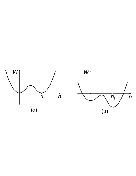
Figure 1: Sample plots of various shapes of the potential $W(n)$. The case (a) corresponds to (2) and is analyzed in this paper.

The potential $W(n)$ in the GL expansion depends upon four parameters ($a,\,b,\,n_{1},\,n_{2}$), two of them (the densities $n_{1}$ and $n_{2}$) are fixed in each phase. The parameters $a$ and $b$ are considered as the free adjustable coefficients of the theory. Supposing slightly more general form of the potential 2, $\tilde{W}(n)=W(n)+\mu(n-n_{1})$, shown in Fig.1b, we may consider the relative difference (RD) between the energy densities in each phase, i.e. the difference between the values at the minima of $\tilde{W}(n)$ (see Fig.1b) as an extra adjustable parameter. It is easy to see that this difference is closely connected to the asymptotic behavior of the solvation energy at large solute sizes. Actually, the RD contributes to the volume–dependent part of the solvation energy. It is obvious that the term which scales linearly with the volume, tends to $\frac{1}{3}PV_{\text{solute}}$ as the solute volume $V_{\text{solute}}$ increases spt (here $P$ is the liquid pressure). However the simple quantitative estimation shows that on the nanometer scale the volume contribution is negligible in comparison with the surface contribution to the solvation energy chand4 . Thus we may neglect the difference in minima of the potential shown in Fig.1b and consider everywhere further the potential symmetric upon the phase change—see Fig.1a. Just such functional form of the potential is proposed above in (2).

We can find the equilibrium densities minimizing the Hamiltonian (1) with respect to the (still decoupled) fields $n({\bf r})$ and $\rho({\bf r})$:

$$\int\chi({\bf r}-{\bf r}^{\prime})\omega({\bf r}^{\prime})\,d{\bf r}^{\prime}=0$$ (4a)

$$-a\Delta n({\bf r})+\frac{\delta W(n({\bf r}))}{\delta n({\bf r})}=0$$ (4b)

In absence of any interactions between the fields $\omega$ and $n$, the solution of (4a) postulates the homogeneity of the liquid $\omega(\mathbf{r})=\text{const}$, while Eq.(4b) describes: a) the plain vapor–liquid interface supplied with the boundary conditions $n(\mathbf{-\infty})\equiv n_{1}=0$ ($n(\mathbf{\infty})=n_{2}$) in the one–dimensional case, and b) the density profile near the surface of extended macroscopic object in the two– and three–dimensional case with boundary conditions $n=0$ at the solute surface and $\mathbf{\nabla}n=0$ for $|\mathbf{r}|\to\infty$. Everywhere further in this Section for simplicity we consider the spherical objects only (the solvation of objects of other shapes is discussed at lengths of the Section III).

Qualitatively these solutions can be analyzed by computing the first integral of motion (as in the classical mechanics ll_1 ). Writing the first term in Eq.(4b) in 3D as $\Delta n(r)=n^{\prime\prime}(r)+\frac{2}{r}n^{\prime}(r)$, multiplying (4b) by $n^{\prime}(r)\equiv\frac{dn(r)}{dr}$ and integrating it from $r_{\rm in}$ (the radius of the sphere) to $\infty$, we obtain:

$$-a\int_{r_{\rm in}}^{\infty}\frac{d}{dr}\left[\frac{(n^{\prime}(r))^{2}}{2}\right]dr-a\int_{r_{\rm in}}^{\infty}\frac{2}{r}(n^{\prime}(r))^{2}dr+\int_{r_{\rm in}}^{\infty}\frac{dW(r)}{dr}dr=0;\qquad n^{\prime}(\infty)=0$$ (5)

Hence, we get from (5) the following relation:

$$(n^{\prime}(r))^{2}\Big{|}_{r=r_{\rm in}}=\int_{r_{\rm in}}^{\infty}\frac{4}{r}(n^{\prime}(r))^{2}dr+\frac{2}{a}[W(n(r_{\rm in}))-W(n(\infty))]$$ (6)

Having the equation (6) and the exact functional form of the potential (2) in hand, we know the value of $n^{\prime}(r)$ at the point $r=r_{\rm in}$ which determines the qualitative behavior of the density profile. In our case the second integrand vanishes, hence the density monotonically increases from $n_{1}$ at the point $\mathbf{r}_{\text{in}}$ to $n_{2}$ for $|\mathbf{r}|=\infty$. In practice, the liquid density reaches quickly the bulk value at some distance outside the solute surface. The analysis of an asymmetric potentials with RD can be performed within the same formalism.

The sense of the parameters $a$ and $b$ becomes transparent in the limit of large spherical solute molecules $r_{\rm in}\gg\delta$, where $\delta$ is the characteristic size of the liquid–vapor interface (see below). Substituting (2) into (4b) and replacing the interaction of the field $n({\bf r})$ with the solute molecule by the boundary condition, we get

$$\left\{\begin{array}[]{l}-a\Delta n({\bf r})+2b(n({\bf r})-n_{\text{avr}})(n({\bf r})-n_{1})(n({\bf r})-n_{2})=0\vskip 6.0pt plus 2.0pt minus 2.0pt\\ n({\bf r}=r_{\rm in})=n_{1}\end{array}\right.$$ (7)

where $\displaystyle{n_{\text{avr}}}=\frac{n_{2}+n_{1}}{2}$. Supposing in (7) that $r\gg\delta$, we can expand the 3D Laplacian

$$\Delta=\left.\frac{d^{2}}{dr^{2}}+\frac{2}{r}\frac{d}{dr}\right|_{r\gg\delta}=\frac{d^{2}}{dr^{2}}+O\left(\frac{\delta}{r}\right)$$

and obtain the effective 1D equation

$$\left\{\begin{array}[]{l}\displaystyle-a\,\tilde{n}^{\prime\prime}(r)+2b\,(\tilde{n}(r)-n_{\text{avr}})(\tilde{n}(r)-n_{1})(\tilde{n}(r)-n_{2})=0\vskip 6.0pt plus 2.0pt minus 2.0pt\\ \tilde{n}(r_{\rm in})=n_{\text{avr}}\end{array}\right.$$ (8)

whose solution reads

$$\tilde{n}(r)=\frac{n_{2}-n_{1}}{2}\tanh\left(\frac{r-r_{\rm in}}{\delta}\right)+\frac{n_{2}+n_{1}}{2};\qquad\delta=\frac{2}{n_{2}-n_{1}}\sqrt{\frac{a}{b}}$$ (9)

It is clear that the symmetric potential of GL form leads to the one–parameter theory. This parameter $\delta$ fixes the width of the phase separation interface. The solvation free energy $\tilde{G}$ per the spherical solute area $4\pi r_{\rm in}^{2}$ in the limit of large molecules can now be expressed as follows

$$\begin{array}[]{lll}\displaystyle\frac{\tilde{G}}{4\pi r_{\rm in}^{2}}&=&\displaystyle\frac{1}{4\pi r_{\rm in}^{2}}\int_{-\delta}^{\delta}\left\{\frac{a}{2}(\nabla\tilde{n})^{2}+\frac{b}{2}(\tilde{n}-n_{1})^{2}(\tilde{n}-n_{2})^{2}\right\}4\pi r^{2}dr\vskip 6.0pt plus 2.0pt minus 2.0pt\\ &=&\displaystyle\frac{\sqrt{ab}}{6}(n_{2}-n_{1})^{3}+O\left(\frac{\delta}{r_{\rm in}}\right)\end{array}$$ (10)

where the coefficient

$$\sigma=\displaystyle\frac{\sqrt{ab}}{6}(n_{2}-n_{1})^{3}$$

has a sense of a surface tension. Note that for $0<\frac{\delta}{r_{\rm in}}\ll 1$ in the leading order of the expansion (10) the true boundary condition $n(r_{\rm in}-\delta)=0$ cannot be distinguished from the approximate one, $n(r_{\rm in})=n_{\text{avr}}$.

II.2 The correlation function

The important component of our model is the bulk correlation function, $\chi(|{\bf r}-{\bf r}^{\prime}|)$, of a solvent. It appears as an input into the theory. Recall some basic facts concerning the function $\chi(|{\bf r}-{\bf r}^{\prime}|)$. We have by definition:

$$\chi(|{\bf r}-{\bf r}^{\prime}|)=\overline{n}\delta({\bf r}-{\bf r}^{\prime})+\overline{n}^{2}h(|{\bf r}-{\bf r}^{\prime}|)$$ (11)

where $\overline{n}$ is the mean solvent density in the bulk, $h({\bf r}-{\bf r}^{\prime})=g({\bf r}-{\bf r}^{\prime})-1$ and the function $g(|{\bf r}-{\bf r}^{\prime}|)$ has very clear physical meaning:

$$n^{2}({\bf r})g({\bf r})=V^{-1}\big{\langle}\sum_{i\neq j}\delta({\bf r}-{\bf r}_{i}+{\bf r}_{j})\big{\rangle}$$ (12)

The function $g({\bf r})$ may be determined from experimental data, or numerical simulations, or, say, from some selfconsistent integral equation with corresponding bridge functional sarkisov .

The following relation is the direct consequence of the definition of $\chi({\bf r}-{\bf r}^{\prime})$:

$$\overline{n}\int\Big{(}g(|{\bf r}-{\bf r}^{\prime}|)-1\Big{)}\,d{\bf r}^{\prime}=4\pi\overline{n}\int h(r)r^{2}dr=-1$$ (13)

The inverse correlation function $\chi_{\rm in}^{-1}({\bf r},{\bf r}^{\prime})$ is defined as follows

$$\left\{\begin{array}[]{rcll}\displaystyle\int_{v_{\rm in}}\,d{\bf r}^{\prime\prime}\chi_{\rm in}^{-1}({\bf r},{\bf r}^{\prime\prime})\chi(|{\bf r}^{\prime\prime}-{\bf r}^{\prime}|)&=&\delta({\bf r}^{\prime}-{\bf r})&\qquad\mbox{for ${\bf r}\in v_{\rm in}$}\vskip 6.0pt plus 2.0pt minus 2.0pt\\ \displaystyle\chi^{-1}_{\rm in}({\bf r},{\bf r}^{\prime\prime})&=&0&\qquad\mbox{for ${\bf r}\in v_{\rm out}$}\end{array}\right.$$ (14)

Let us pay attention that the integration in (14) is spread only to the volume $v_{\rm in}$ occupied by the solute and hence the function $\chi_{\rm in}^{-1}({\bf r},{\bf r}^{\prime})$ is not translationally invariant.

We have used in our work two different correlation functions: i) the correlation function of water obtained from the numerical molecular–dynamical simulations corr_water , and ii) the correlation function of hard spheres constructed on the basis of solution of self–consistent integral equation completed by the Percus-Yevic bridge functional py ; PYanalyt . The functions $h(|{\bf r}-{\bf r}^{\prime}|)=g(|{\bf r}-{\bf r}^{\prime}|)-1$ of water and of hard sphere liquid are shown in Fig.2. Both functions correspond to the dimensionless bulk density $n_{2}=0.7$. Some approximate equations of the theory of liquids in the statistical thermodynamics of classical liquid systems one can find, for instance, in the review article sarkisov .

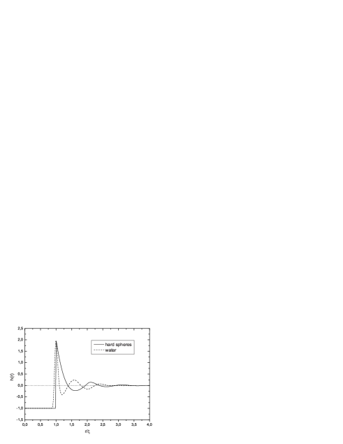
Figure 2: Correlation function of water vs Percus–Yevic correlation function of hard spheres. The distance is measured in dimensionless units $r/\xi$ ($\xi=2.78$ Å), the dimensionless bulk density is $n_{2}=0.7$.

Working simultaneously with two different correlation functions (of water and of hard spheres) we able able to check the sensitivity of the physical observable quantities (as the density and the free energy) to the details of the correlation function, as well as to verify the convergence of our numerical scheme: far away from the solute surface the results of computations should not be sensitive to the particular choice of the correlation function.

The correlation function defines the natural scale, $\xi$, in the theory. In what follows we fix $\xi=2.78$ Å  as the distance till the first peak in the correlation function of water.

II.3 The partition function

Now we turn to the solute–solvent interactions. To take into account the effect of the solute solvation, we demand the total density $\rho$ to be zero inside the volume $v_{\rm in}$ of the solute:

$$\rho({\bf r})=n({\bf r})+\omega({\bf r})\equiv 0$$ (15)

where ${\bf r}\in v_{\rm in}$. The direct interaction between the short– and the long–range density fluctuations in the solvent can be written in the simplest possible way

$$V[\omega,n]=c\int{\omega}({\bf r})\,n({\bf r})\,d{\bf r}$$ (16)

where $c$ is the coupling constant. In what follows all the analytic derivations are performed for generic $c$, however the numerical solutions of the corresponding equations are presented for $c=0$ only. The case $c\neq 0$ we leave for the future consideration.

The solute–solvent partition function is obtained as follows

$$Z=\int\mathcal{D}\{\omega({\bf r})\}\prod_{{\bf r}\in V_{\rm in}}\delta\left[\rho({\bf r})\right]e^{-\mathcal{H}}$$ (17)

where

$$\mathcal{H}=\mathcal{H}_{0}[\omega,n]+V[\omega,n]+\int\,d\mathbf{r}\,\varphi(\mathbf{r})\rho(\mathbf{r})$$ (18a)

$$\rho({\bf r})=n({\bf r})+\omega({\bf r})$$ (18b)

Let us rewrite the constraints imposed by the Dirac $\delta$–function in (17) using the functional Fourier transform

$$\prod_{{\bf r}\in v_{\rm rm}}\delta\left[\rho({\bf r})\right]=\frac{1}{(2\pi)^{\mathcal{N}}}\int\mathcal{D}\{\psi({\bf r})\}\exp\left\{i\int_{v_{\rm in}}\rho({\bf r})\,\psi({\bf r})\,d{\bf r}\right\}$$ (19)

where $\mathcal{N}$ is the number of points in the product $\prod\limits_{{\bf r}\in v_{\rm in}}(...)$, and we have denoted $\mathcal{D}\{\psi({\bf r})\}\equiv\prod\limits_{{\bf r}\in v_{\rm in}}d\psi({\bf r})$. Now we can represent the partition function $Z[\varphi({\bf r})]$ in (17) as a functional integral over an auxiliary field $\psi({\bf r})$:

$$\begin{array}[]{r}\displaystyle Z=\Xi^{-1}\int\mathcal{D}\{\omega({\bf r})\}\mathcal{D}\{\psi({\bf r})\}e^{-S[\omega,n,\psi]}\vskip 6.0pt plus 2.0pt minus 2.0pt\\ \displaystyle S[\omega,n,\psi]=\mathcal{H}[\omega,n]+i\int_{v_{\rm in}}\rho({\bf r})\,\psi({\bf r})\,d{\bf r}\end{array}$$ (20)

where $\Xi$ is some physically irrelevant constant which defines the normalization of the partition function $Z$.

The partition function $Z$ with the action $S[\omega,n,\psi]$ defined in (20) is the key object for our computations. Such quantities as the total, $\rho({\bf r})$, and the averaged, $n({\bf r})$, densities, the solvation free energy, $\Delta G$, the free energy of interactions of different solute molecules in the solvent, etc. can be calculated on the basis of the generating function $Z$.

II.4 The mean density

To define the mean (large scale) density $n(r)$, let us require

$$\frac{\delta S[n({\bf r})]}{\delta n({\bf r})}=0$$ (21)

In (21) all other fields except $n({\bf r})$ are supposed to be already integrated over. This leads to the functional equation which can be written explicitly as a set of two coupled integro–differential equations relating the inner (${\bf r}\in v_{\rm in}$) and outer (${\bf r}\in v_{\rm out}$) regions of the solute molecule:

$$\begin{array}[]{ll}\displaystyle-a\Delta n({\bf r})+\frac{\delta W(n({\bf r}))}{\delta n({\bf r})}-2cn({\bf r})-&\vskip 6.0pt plus 2.0pt minus 2.0pt\\ \displaystyle c\int_{v_{\rm in}}d{\bf r}^{\prime}\int_{v_{\rm out}}d{\bf r}^{\prime\prime}\chi^{-1}_{\rm in}({\bf r},{\bf r}^{\prime})\chi(|{\bf r}^{\prime}-{\bf r}^{\prime\prime}|)n({\bf r}^{\prime\prime})+\int_{v_{\rm in}}d{\bf r}^{\prime}\chi^{-1}_{\rm in}({\bf r},{\bf r}^{\prime})n({\bf r}^{\prime})=0&\qquad\mbox{for ${\bf r}\in v_{\rm in}$}\end{array}$$ (22a)

and

$$\begin{array}[]{ll}\displaystyle-a\Delta n({\bf r})+\frac{\delta W(n({\bf r}))}{\delta n({\bf r})}-c^{2}\int_{v_{\rm out}}d{\bf r}^{\prime}\chi(|{\bf r}-{\bf r}^{\prime}|)n({\bf r}^{\prime})+\vskip 6.0pt plus 2.0pt minus 2.0pt\\ \displaystyle c^{2}\int_{v_{\rm in}}d{\bf r}^{\prime}\int_{v_{\rm in}}d{\bf r}^{\prime\prime}\int_{v_{\rm out}}d{\bf r}^{\prime\prime\prime}\chi(|{\bf r}-{\bf r}^{\prime}|)\chi^{-1}_{\rm in}({\bf r}^{\prime},{\bf r}^{\prime\prime})\chi(|{\bf r}^{\prime\prime}-{\bf r}^{\prime\prime\prime}|)n({\bf r}^{\prime\prime\prime})-&\vskip 6.0pt plus 2.0pt minus 2.0pt\\ \displaystyle c\int_{v_{\rm in}}d{\bf r}^{\prime}\int_{v_{\rm in}}{\bf r}^{\prime\prime}\chi(|{\bf r}-{\bf r}^{\prime}|)\chi^{-1}_{\rm in}({\bf r}^{\prime},{\bf r}^{\prime\prime})n({\bf r}^{\prime\prime})=0&\qquad\mbox{for ${\bf r}\in v_{\rm out}$}\end{array}$$ (22b)

In the current paper we pay attention to the case $c=0$ only, i.e. when the direct coupling between the short– and long–ranged fluctuation is absent. In that case the profiles of the mean density $n(r)$ for spherical solute molecules of different sizes are given by the solutions of the simplified integro–differential equation

$$-a\Delta n({\bf r})+\frac{\delta W(n({\bf r}))}{\delta n({\bf r})}+\int_{v_{\rm in}}d{\bf r}^{\prime}\chi^{-1}_{\rm in}({\bf r},{\bf r}^{\prime})n({\bf r}^{\prime})=0 {\bf r}\in v_{\rm in}$$ for (23a)

$$\displaystyle-a\Delta n({\bf r})+\frac{\delta W(n({\bf r}))}{\delta n({\bf r})}=0 {\bf r}\in v_{\rm out}$$ for (23b)

We solve (23a)–(23b) numerically by using the simple technical trick which allows to increase essentially the speed of the computations. Namely, we have observed that the most CPU time is spent for the calculation of $\chi^{-1}_{\rm in}({\bf r},{\bf r}^{\prime})$ on the basis of (14). To get rid of this part of computations we can multiply the (23a) by $\chi(|{\bf r}-{\bf r}^{\prime}|)$ and integrate over the whole space $v_{\rm tot}$ ($v_{\rm tot}=v_{\rm in}\cup v_{\rm out}$), with the subsequent application of (14). Finally we arrive at the following set of equations:

$$\begin{array}[]{rl}\displaystyle n({\bf r})+\int_{v_{\rm in}}d{\bf r}^{\prime}\chi(|{\bf r}-{\bf r}^{\prime}|)\left(-a\Delta n({\bf r}^{\prime})+\frac{\delta W(n({\bf r}^{\prime}))}{\delta n({\bf r}^{\prime})}\right)=0&\qquad\mbox{for ${\bf r}\in v_{\rm in}$}\vskip 6.0pt plus 2.0pt minus 2.0pt\\ \displaystyle-a\Delta n({\bf r})+\frac{\delta W(n({\bf r}))}{\delta n({\bf r})}=0&\qquad\mbox{for ${\bf r}\in v_{\rm out}$}\end{array}$$ (24)

The generic form of the mean density profile $n(r)$ for the spherical solute molecule is shown in Fig.3 for different (still arbitrary) values of the constants $a$ and $b$ of Hamiltonian. The densities of the vapor ($n_{1}$) and bulk ($n_{2}$) phases are as follows: $n_{1}=0;\,n_{2}=0.7$. The numerical solutions of (24) are obtained with the correlation functions of hard spheres (dashed line) and of water (solid line). The typical plots are shown in Fig.3.

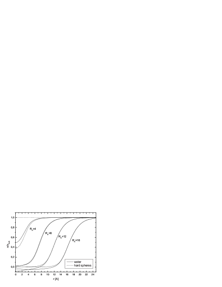
Figure 3: Typical profiles of the mean density $n(r)$ around spherical solute molecules of different radii $R_{\bf in}$.

The presence of the regions with the negative values of the mean densities in the vapor phase should not confuse—remember that only the full density $\rho({\bf r})$ is a conserved value and should be zero inside the solute molecule, while the average density $n({\bf r})$ is determined selfconsistently. The existence of the regions with negative values of the long–ranged averaged field $n({\bf r})$ signifies that in these regions the fluctuations of the short–ranged field $\rho({\bf r})$ are not symmetric, such that locally $\left<\omega\right>\neq 0$. Such regions exist only inside the solute volume $v_{\rm in}$ and in the ”physical” volume $v_{\rm out}$ (i.e. outside the solute) the mean density is always positive.

The full density $\rho({\bf r})=n({\bf r})+\omega({\bf r})$ which minimizes the functional (20) satisfies the following set of equation

$$\begin{array}[]{llll}\rho(\mathbf{r})&=&0,&\qquad\mbox{for ${\bf r}\in v_{\rm in}$}\vskip 6.0pt plus 2.0pt minus 2.0pt\\ \rho(\mathbf{r})&=&\displaystyle n(\mathbf{r})-\int_{v_{\rm in}}d\mathbf{r}^{\prime}\int_{v_{\rm in}}d\mathbf{r}^{\prime\prime}\chi(|\mathbf{r}-\mathbf{r}^{\prime}|)\chi^{-1}_{\text{in}}(\mathbf{r}^{\prime},\mathbf{r}^{\prime\prime})n(\mathbf{r}^{\prime\prime})+&\vskip 6.0pt plus 2.0pt minus 2.0pt\\ &&\displaystyle c\int_{v_{\rm in}}d\mathbf{r}^{\prime}\int_{v_{\rm in}}d\mathbf{r}^{\prime\prime}\int_{v_{\rm in}}d\mathbf{r}^{\prime\prime\prime}\chi(|\mathbf{r}-\mathbf{r}^{\prime}|)\chi^{-1}_{\text{in}}(\mathbf{r}^{\prime},\mathbf{r}^{\prime\prime})\chi(|\mathbf{r}-\mathbf{r}^{\prime\prime\prime}|)n(\mathbf{r}^{\prime\prime\prime})-&\vskip 6.0pt plus 2.0pt minus 2.0pt\\ &&\displaystyle c\int_{v_{\rm out}}d\mathbf{r}^{\prime}\chi(|\mathbf{r}-\mathbf{r}^{\prime}|)n(\mathbf{r}^{\prime})&\qquad\mbox{for ${\bf r}\in v_{\rm out}$}\end{array}$$ (25)

The equations (25) with $c=0$ again can be rewritten in the form which excludes the function $\chi^{-1}_{\text{in}}(\mathbf{r},\mathbf{r}^{\prime})$ from the corresponding expressions.

II.5 The solvation free energy

The free energy of solvation $\Delta G$ is defined as the energy necessary to transport the solute molecule from its environment in the solvent to the vacuum. The partition functions of solvent samples of sufficiently large volume $V_{\rm solvent}$ containing the solute molecule inside can be straightforwardly written on the basis of (17):

$$Z_{\rm solvent-solute}=\int_{v_{\rm solvent}}\mathcal{D}\{\omega({\bf r})\}\prod_{{\bf r}\in v_{\rm solute}}\delta\left[\rho({\bf r})\right]e^{-\mathcal{H}}$$ (26)

where $\mathcal{H}$ is given by (18a). Conventionally the solvation free energy $\Delta G$ is written as follows

$$\Delta G=-\ln\frac{Z_{\rm solvent-solute}}{Z_{\rm solvent\;only}}$$ (27)

where $Z_{\rm solvent\;only}$ is the partition function of the pure solvent (without the solute molecules). At first glance it seems naturally to write $Z_{\rm solvent\;only}$ simply as

$$Z_{\rm solvent\;only}=\int_{v_{\rm solvent}}\mathcal{D}\{\omega({\bf r})\}\,e^{-\mathcal{H}}$$ (28)

However the expression (28) being used in (27) leads to the divergence of the solvation free energy $\Delta G$ in practical computations based on the approach developed in (17)–(24). The formal reason for such a divergence deals with the occurrence of uncompensated infinite product of Gaussian integrals (20) in the ratio $Z_{\rm solvent-solute}/Z_{\rm solvent\;only}$ in (27). The physical origin of such a divergence is due to the mixture of different statistical ensembles associated with the partition functions (26) and (28). Namely, when writing $Z_{\rm solvent-solute}$ as in (26) and imposing the $\delta$–function constraint, we fix some particular value of the field $\rho$ within the solute volume $v_{\text{in}}$ what means that (26) is the partition function of the canonical ensemble (with respect to the density $\rho$). At the same time, for $Z_{\rm solvent\;only}$ written in the form (28), we allow any density of the field $\rho$ inside the solute volume. Hence, (28) is the partition function of the grand canonical ensemble.

The regularization of eq.(28) is based on the probabilistic consideration of the solvation free energy chand2 . Rewrite $\Delta G$ in (27) as follows

$$\Delta G=-\ln\frac{Z_{v}(0)}{\sum_{N\geq 0}Z_{v}(N)}$$ (29)

where $Z_{v}(N)$ is a partition function of $N$ molecules inside the volume $v_{\rm in}$. The continuous analog of the last expression appears when passing from $N$ to the average number of molecules $\tilde{n}=N/v_{\rm in}$. Simultaneously we require the net density $\rho$ to be equal $\tilde{n}$ inside $v_{\rm in}$ and replace the summation over $N$ by the integration over $\tilde{n}$. Now we can rewrite the normalization partition function $Z_{\rm solvent\;only}$ in the following ”regularized” form

$$Z_{\rm solvent\;only}=\int_{0}^{\infty}d\tilde{n}\int_{v_{\rm solvent}}\mathcal{D}\{\omega({\bf r})\}\prod_{{\bf r}\in v_{\rm solute}}\delta\left[\rho({\bf r})-\tilde{n}\right]\,e^{-\mathcal{H}}$$ (30)

Instead of this form we use an approximation

$$Z_{\rm solvent\;only}=\int_{v_{\rm solvent}}\mathcal{D}\{\omega({\bf r})\}\prod_{{\bf r}\in v_{\rm solute}}\delta\left[\rho({\bf r})-\bar{n}\right]\,e^{-\mathcal{H}}$$ (31)

obtained from (30) by the stationary phase integral calculation technic. Thus, the definition (27) with the partition functions given by (26) and (31) is very natural, justified physically and does not contain any divergences. It is important to notice that the computation of the equilibrium density based on $Z_{\rm solvent\;only}$ given by (30) is the bulk density, for which the value of corresponding effective Hamiltonian is strictly zero.

The solvation free energy $\Delta G$ for any solute molecule is computed on the basis of the equilibrium density profile $n_{\rm eq}({\bf r})\equiv n({\bf r})$ calculated from Eqs.(22a)–(22b). Substituting $n_{\rm eq}({\bf r})$ back into the Hamiltonian (18a) and taking into account (14), we can rewrite the solvation free energy $G\equiv\mathcal{H}\{n_{\rm eq}\}$ as a sum of three terms:

$$\Delta G_{\rm solv}(v_{\rm in})=\Delta G_{\rm corr}+\Delta G_{\rm surf}+\Delta G_{\rm int}$$ (32)

where

$$\begin{array}[]{lll}\Delta G_{\rm corr}&=&\displaystyle\frac{1}{2}\int_{v_{\rm in}}n_{\rm eq}({\bf r})\chi_{\rm in}^{-1}({\bf r},{\bf r}^{\prime})n_{\rm eq}({\bf r}^{\prime})\,d{\bf r}d{\bf r}^{\prime}\vskip 6.0pt plus 2.0pt minus 2.0pt\\ \Delta G_{\rm surf}&=&\displaystyle\frac{a}{2}\int(\nabla n_{\rm eq}({\bf r}))^{2}d{\bf r}\vskip 6.0pt plus 2.0pt minus 2.0pt\\ \Delta G_{\rm int}&=&\displaystyle\int W\left(n_{\rm eq}({\bf r})\right)d{\bf r}\end{array}$$ (33)

As in the computations of the mean density $n(r)$, here we consider the case $c=0$ only. In that case (32) can be rewritten in the following form

$$\Delta G_{\rm solv}(v_{\rm in})=\int_{v_{\rm in}}\left(W(n)-\frac{n}{2}\frac{\delta W}{\delta n}\right)d\mathbf{r}$$ (34)

The contributions to the normalized solvation free energy

$$\Delta\tilde{G}_{\rm solv}=\frac{\Delta G_{\rm solv}}{4\pi r_{\rm in}^{2}}$$ (35)

of a spherical solute molecule of radius $R$ are shown in Fig.4 for each term $\{\Delta\tilde{G}_{\rm corr}$, $\Delta\tilde{G}_{\rm surf}$, $\Delta\tilde{G}_{\rm int}\}=\{\Delta G_{\rm corr}$, $\Delta G_{\rm surf}$, $\Delta G_{\rm int}\}/(4\pi R_{\rm in}^{2})$ separately, as well as for the sum $\Delta\tilde{G}_{\rm solv}=\Delta\tilde{G}_{\rm corr}+\Delta\tilde{G}_{\rm surf}+\Delta\tilde{G}_{\rm int}$. The diameter of the solvent molecule in Fig.4 is set to 1.

Figure 4: Typical behavior of the solvation free energy for different choice of parameters $a$ and $b$ in the Hamiltonian (left); Contributions to the normalized solvation free energy $\Delta\tilde{G}_{\rm solv}(R_{\rm in})$ of a spherical solute from $\Delta\tilde{G}_{\rm corr}$, $\Delta\tilde{G}_{\rm surf}$ and $\Delta\tilde{G}_{\rm int}$ for $a=9,\,b=30$ (right).

The solvation free energy of a spherical solute molecule in absence of electrostatic interactions chand1 ; chand2 ; chand3 is proportional (as expected) to the volume of solute molecule for sufficiently small sizes $R_{\rm in}$ (of order of the correlation length in the solvent) and tends to be proportional to the surface area for large $R_{\rm in}$. We clearly see the non-monotonic behavior of the solvation energy upon the size of a solute molecule reported in some works (see, for example, chand4 ).

II.6 Adjustment of the parameters of the Hamiltonian

The free parameters $a$ and $b$ of the Hamiltonian (1)–(2) are chosen from two basic requirements:

i) The theoretically computed normalized solvation free energy $\Delta\tilde{G}_{\rm solv}=\Delta G_{\rm solv}/(4\pi R^{2})$ of a spherical solute molecule of a radius $R$ (see (35)) reproduces the corresponding dependence $\Delta\tilde{G}_{\rm solv}(R)$ obtained in the Monte–Carlo simulations of chand4 ;

ii) The theoretically computed full density $\rho(r|R)$ for few sizes $R$ of spherical solute molecules (25) reproduces the behavior $g(r)$ of the correlation function in vicinity of the spherical solute of radius $R$ extracted from the Monte–Carlo simulations chand4 .

The corresponding results are shown in Fig.5 for the following choice of the parameters: $a=9;\,b=30$.

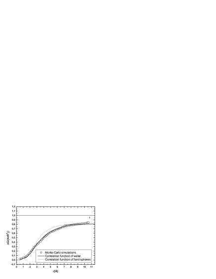
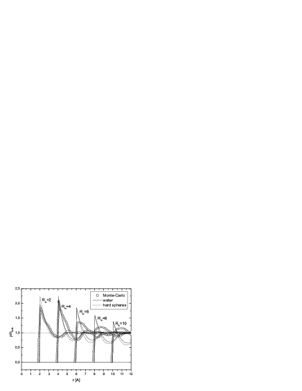
Figure 5: Solvation free energy (34) of a spherical solute vs Monte–Carlo simulations chand4 (left); Profiles of the full density $\rho(r)$ around spherical solutes of different radii $R$ vs Monte–Carlo simulations chand4 for the correlation function $g(r)$.

The dashed and solid lines represent the results obtained with the correlation functions of hard spheres and of the water correspondingly. The solvation energy $\Delta\tilde{G}_{\rm solv}$ is represented in Fig.5 in dimensionless units $\Delta\tilde{G}_{\rm solv}/\gamma$, where $\gamma$ is the surface tension of the flat vapor–water interface. The numerical value $\gamma\approx 72$ mJ/m² is taken from chand4 .

The solvation energies $\Delta G_{\rm solv}$ and $\Delta\tilde{G}_{\rm solv}$ computed directly using (34) and (35) can be converted to the proper units by means of the following scaling coefficients:

$$\left\{\begin{array}[]{l}\displaystyle\Delta G_{\rm solv},\,[\mbox{dimensionless units}]\times 0.2479=\Delta G_{\rm solv},\,[\mbox{kcal/mol}]\vskip 6.0pt plus 2.0pt minus 2.0pt\\ \displaystyle\Delta\tilde{G}_{\rm solv},\,[\mbox{dimensionless units}]\times\frac{0.2479}{(2.78)^{2}}=\Delta\tilde{G}_{\rm solv},\,[\mbox{kcal/(mol \AA${}^{2}$)}]\end{array}\right.$$ (36)

These transfer coefficients remain unchanged in all further computations. In Fig.4 and Fig.5 the radius of a solute molecule is measured in Angstroms.

III Results and discussions: Solvation of objects of various shapes

The current mean–field–type theory of solvation is applied to computation of solvation of neutral molecules (alkanes), as well as to the computation of the free energy of interactions of separated objects (spheres).

III.1 Solvation of alkanes

The parameters of the theory and the scaling coefficient are adjusted to satisfy the Monte–Carlo simulations of solvation of hard spheres and the corresponding profile of the solvent density near the solvated object (see the previous Section) and are not tuned anymore. In particular, we use the same parameters to compute analytically the solvation free energy of alkanes. As it is shown below, we find very good coincidence of our computed values with the predictions of the ”Scaled Particle Theory” which uses the parameters tuned especially to alkanes irisa .

The mentioned coincidence needs some elucidations. There is a viewpoint lee ; widom ; levy supported by numerical computations that one can split the interaction between the solute and the solvent into two parts: i) the free energy, $\Delta G_{\rm cav}$, of a ”cavity formation”, and ii) the dispersion (attractive) part of the Van-der-Waals interactions, $\Delta G_{\rm disp}$. The numerical methods involving the ”thermodynamic integrations” allow to compute both the contributions, $\Delta G_{\rm cav}$ and $\Delta G_{\rm disp}$ separately levy . These contributions can be also computed separately in the frameworks of the ”Scaled Particle Theory” (SPT) developed in spt ; spt1 . The corresponding description of alkanes has been undertaken in irisa where the authors have reported very good quantitative agreement of the sum $\Delta G_{\rm cav}+\Delta G_{\rm disp}$ with the experimentally measured solvation free energy.

The model described in the previous sections of our work considers the solute as an object bounded by hard walls and hence takes into account only the ”cavitation” part of the solvation free energy. The attractive part of the Van-der-Waals interactions is not yet taken into account. However we do not see any principal obstacles in adding the dispersion part of solute–solvent interactions to our model. Moreover, we can ”smear” the $\delta$–functional constraint in (19), releasing more realistic form of the Van-der-Waals potential. The corresponding computations are in progress and will be reported in a forthcoming publication sineta .

The comparison of our predictions for the cavitation part of the solvation free energy of alkanes with the corresponding contribution $\Delta G_{\rm cav}$ extracted from the papers irisa and pais is shown in the table below.

alkanes	$\Delta G_{\rm cav}$, kcal/mol (our model)	$\Delta G_{\rm cav}$, kcal/mol (from irisa )	$\Delta G_{\rm cav}$, kcal/mol (from pais )
${\rm CH_{4}}$	5.69	5.61	5.36
${\rm C_{2}H_{6}}$	7.54	7.53	7.15
${\rm C_{3}H_{8}}$	9.07	9.13
${\rm C_{4}H_{10}}$	10.52	10.8
${\rm C_{5}H_{12}}$	11.96	12.8
${\rm C_{6}H_{14}}$	13.24	14.8	14.22

Table 1: Comparison of the ”cavity formation” contribution, $\Delta G_{\rm cav}$, to the solvation free energy of alkanes computed on the basis of our model with the corresponding data extracted from the papers irisa and pais .

Let us remind once more that in our model the parameters of the Hamiltonian $a=9$, $b=30$ and the scaling factors (36) are tuned on the basis of the Monte–Carlo simulations of solvation of hard spheres without any additional adjustment to alkanes. The volume $v_{\rm in}$ occupied by the alkane molecules we compute using the following prescription. We take the coordinates of centers of all atoms from a standard database, then we draw the spheres with the effective radii 3.5 Å  for all carbon atoms (the length of the C–O bond in water) and 3.05 Å  for all hydrogen bonds (the length of the O–H bond in water) and find $v_{\rm in}$ as the union of the corresponding spherical volumes. The corresponding numerical values of C–O and O–H bonds are extracted from the Monte–Carlo (MC) simulations of the sytemem consisting of 216 water molecules and one methane molecule and subsequent computations of the pairwise correlation functions [C(methane)–O(water)] and [H(methane)–O(water)], ozrin . The same parameters can be extracted using the force field developed in halgren .

As it has already been mentioned above, the dispersion part of the Van-der-Waals (VdW) interaction can be easily taken into account. In the presence of the attractive contribution to the VdW interactions, we should add an extra term $U_{\rm disp}$ to the mean–field potential (1), where

$$U_{\rm disp}=\int U({\bf r})\,n({\bf r})d{\bf r}$$

and $U({\bf r})$ is the attractive part of the VdW interactions.

In the presence of the potential $U({\bf r})$ the equations (23a)–(23b) for the equilibrium mean density are modified in the following simple way: (23a) reminds without changes, while the equation (23b) acquires an additional contribution from the attractive part of the potential $U({\bf r})$ in the region ${\bf r}\in v_{\rm out}$:

$$-a\Delta n({\bf r})+\frac{\delta W(n({\bf r}))}{\delta n({\bf r})}+U({\bf r})=0$$ (37)

III.2 Solvation of cylinders and the free energy of interactions of two separated spheres

In this section we consider the cavitation part of the solvation free energy of molecules of cylindrical geometry, as well as of the free energy of interaction of two hard spheres in the fluctuating media (i.e. in water). Schematically the studied systems are shown in Fig.6. The purpose of this section is two–fold.

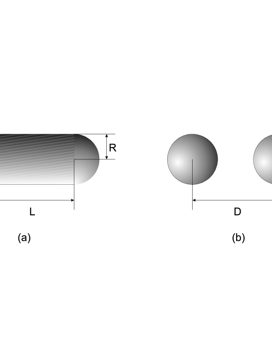
Figure 6: Schematic pictures: of a solvated cylinder ended by two semi-spheres (a), and of two spherical solute molecules (b).

1. First of all, we compute the depth of the ”skin layer” of the solvated object. The naive computation of the solvation free energy (as well as of the free energy of interactions) of large molecules like ligands and proteins demands essential computational resources. Actually, according to (24) one has to take into account the interactions of the fluctuating density field $n({\bf r})$ with all points inside the solvated object $v_{\rm in}$. However it is clear that due to the hard wall constraint the fluctuating field $n({\bf r})$ cannot penetrate deep inside the body of a solute. Considering the solvation of cylindric molecules of different widths and lengths, we study the penetration depth of the density field $n({\bf r})$ inside the solute molecule.

The dependence of the solvation free energy $\Delta G_{\rm cyl}(L|R)$ upon its length $L$ for two different radii $R$ is shown in Fig.7a.

Figure 7: (a) Solvation free energy $\Delta G_{\rm cyl}(L|R)$ of a cylinder as a function of its length $L$ for different $R$ in the range $R=0.9...1.5$; (b) Slope of $\Delta G_{\rm cyl}(R)$ as a function of $R$ at $L=12$ Å.

As one sees, from Fig.8b, the slope of the curves in Fig.7 becomes constant approximately for $R>R_{0}\approx 1.4\xi=3.9$ Å. It means that for $R>R_{0}$ the fluctuating density field penetrates inside the body of the solute to some fixed length only (to the depth of the ”skin layer”). Hence, we may not account of all internal points of the solute located into its body beyond the skin layer $R_{0}\approx 3.9$ Å.

2. Secondary, we investigate the free energy of interaction $\Delta G_{\rm sph}=\Delta G_{\rm sph\,int}(D|R)-\Delta G_{\rm sph\,solv}(D\to\infty|R)$ of two spherical solute molecules, each of radius $R$, upon the distance $D$ between their centers. The free energy of interaction, or ”the mean force potential” dill ; shi $\Delta G_{\rm sph}(D|R)$, with the subtracted solvation energies of two solitary spheres, is computed for the hard–core potential, $U(D)$, where

$$U(D)=\left\{\begin{array}[]{ll}\infty&\mbox{for $D\leq 2R$}\vskip 6.0pt plus 2.0pt minus 2.0pt\\ 0&\mbox{for $D>2R$}\end{array}\right.$$

i.e. we again take into account only the cavitation part of the free energy of interactions, neglecting the dispersion (attractive) part of the direct Van-der-Waals interactions between the impenetrable spheres of radius $R$.

Even for such simplified situation we have found that the behavior of $\Delta G_{\rm sph}(D|R)$ on $D$ is qualitatively different for different values of $R$ compared to $\xi$ . Let us stress once more that $\Delta G_{\rm sph}$ is the free energy of interaction between two spheres with the subtracted solvation energies of two solitary spheres $\Delta G_{\rm sph\,solv}(D\to\infty|R)$. The observed dependencies are shown in Fig.8.

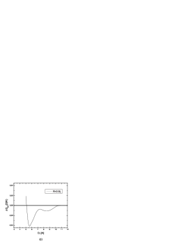
Figure 8: Free energy of interactions $\Delta G_{\rm sph}$ of two spherical solute molecules as a function of the distance between their centers $D$ for $R=0.4\xi$ (a); $R=0.7\xi$ (b) and $R=0.9\xi$ (c).

For all radii, $R=0.4\xi$ Å , $0.7\xi$ Å  and $0.9\xi$ Å  we reproduce the non-monotonic dependence $\Delta G_{\rm sph}(D)$ on $D$. This non-monotonicity is the manifestation of the oscillatory behavior of the water correlation function. Such behavior has been found earlier in direct numerical simulations consistent with the predictions of the ”Scaled Particle Theory” (see dill and the references therein), and on the basis of estimation of the solvent accessible surface area shi . The account of the Van-der-Waals attractive tail in the potential $U(D)$ can essentially change the behavior $\Delta G_{\rm sph}(D)$, however the non-monotonic behavior $\Delta G_{\rm sph}(D)$ will still hold.

Comparing Fig.8a and Fig.8c, we see that the dependence $\Delta G_{\rm sph}(D)$ is sensitive (even qualitatively) to the size $R$ of interacting spheres. The effective attraction between smaller spheres is weaker than that of larger spheres. This effect can be easily understood. For sufficiently large spheres, $R\gtrsim\xi$, there is an penalty in the free energy of keeping two solute molecules close to each other, which is the ”classical manifestation” of the Casimir–type effect. At the same time, the sufficiently small solute molecules (with $R\lesssim\xi$) are located in spontaneously created fluctuational cavities of size $\xi$ in water and the penalty for expelling the water from the volume occupied by two solute molecules close to each other is essentially smaller than that for large solutes. Moreover, one can see from Fig.8a that the mean force potential has the attractive (negative) part corresponding to the second water shell only. So, the two sufficiently small spherical solutes can form a bound state separated by one water shell. The found behavior qualitatively coincides with the results of the work dill , where the authors have studied the ”potential of the mean force” acting between two spherical solute molecules.

III.3 Electrostatics in fluctuating dipolar environment

There are different ways to implement the electrostatic interactions into our self–consistent mean–field description. In many works it is assumed that the dielectric permittivity of the solvent, $\varepsilon$, linearly depends on the solvent density, $n({\bf r})$, i.e., $\varepsilon({\bf r})=1+\alpha\,n({\bf r})$. In our approach we get rid of such supposition and follow the self–consistent scheme where the solvent is considered as a ”gas” of dipoles. Our method ideologically is very close to the consideration of the Debye screening in electrically neutral plasma ll_5 . However, to the contrast with plasma, in our case the positive and negative ions are connected by holonomic constraints in pairs, forming the short–ranged dipoles. The screening in the system of extended objects was a subject of many investigations. The description, most appropriate for our goals, has been developed in the appendix of the paper khkh .

Below we derive the basic set of equations describing simultaneously electrostatic and hydrophobic interactions in the fluctuating media. The detailed analysis of the obtained equations together with the numerical computation of the free energies of solvation and interactions of charged molecules, will be the subject of the forthcoming publication sineta , while here we analyze briefly the limiting case, in which the proposed theory coincides with the electrostatics in the continuous media with some effective density–dependent permittivity $\varepsilon({\bf r})$.

Let us introduce the quantities:

$\rho_{\rm mol}^{q}({\rm r},\tau)$ – the charge distribution of the solvent molecule with the orientation $\tau$ and with the center of mass situated at the point ${\bf r}$. Outside of the molecule $\rho_{\rm mol}^{q}({\bf r},\tau)=0$;

$\rho_{\rm solute}^{q}({\bf r})$ – the charge distribution of the solute;

$\phi_{\rm eff}({\bf r})$ – the effective mean electrostatic field.

Sticking to the mean–field description developed in khkh , we can place each solvent molecule in a self–consistent field electrostatic field, $\phi(\mathbf{r})$, averaged over the volume of this solvent molecule. So, we have:

$$\phi(\mathbf{r},\tau)=\int\phi_{\rm eff}({\bf r}^{\prime})\rho_{\rm mol}^{q}({\bf r}^{\prime}-{\bf r},\tau)\,d{\bf r}^{\prime}$$ (38)

The electrostatic potential $\phi_{\text{eff}}(\mathbf{r})$ is determined by the Poisson equation

$$\Delta\phi_{\text{eff}}(\mathbf{r})=-\frac{4\pi}{\varepsilon_{\text{solute}}}\rho_{\text{solute}}^{q}(\mathbf{r})-\mu(\mathbf{r})$$ (39)

where $\mu(\mathbf{r})$ is the media charge density

$$\mu(\mathbf{r})=\int\int\left(e^{-\beta\phi(\mathbf{r}^{\prime},\tau)}-1\right)\rho_{\text{mol}}^{q}(\mathbf{r}-\mathbf{r}^{\prime},\tau)\rho(\mathbf{r}^{\prime})\frac{d\Omega_{\tau}}{4\pi}d^{3}\mathbf{r}^{\prime}$$ (40)

and $\rho(\mathbf{r})=n(\mathbf{r})+\omega(\mathbf{r})$ is the solute density. Neglecting the short–range fluctuations, $\omega(\mathbf{r})$ we may write in the mean–field approximation

$$\mu(\mathbf{r})=\int\int\left(e^{-\beta\phi(\mathbf{r}^{\prime},\tau)}-1\right)\rho_{\text{mol}}^{q}(\mathbf{r}-\mathbf{r}^{\prime},\tau)n(\mathbf{r}^{\prime})\frac{d\Omega_{\tau}}{4\pi}d^{3}\mathbf{r}^{\prime}$$ (41)

The full Hamiltonian of the system reads now:

$$\begin{array}[]{lll}H[n(\mathbf{r}),\phi_{\text{eff}}(\mathbf{r})]&=&\displaystyle\int d\mathbf{r}\,\left(\frac{a}{2}(\nabla n(\mathbf{r}))^{2}+W(n)\right)+\frac{1}{2}\int_{v_{\text{in}}}d\mathbf{r}\,d\mathbf{r}^{\prime}\,n(\mathbf{r})\chi^{-1}_{\text{in}}(\mathbf{r},\mathbf{r}^{\prime})n(\mathbf{r}^{\prime})\vskip 6.0pt plus 2.0pt minus 2.0pt\\ &+&\displaystyle\lambda\int d\mathbf{r}\,(\nabla\phi_{\text{eff}}(\mathbf{r}))^{2}+\int d\mathbf{r}\,\varphi(\mathbf{r})\left(\Delta\phi_{\text{eff}}(\mathbf{r})+\frac{4\pi}{\varepsilon_{\text{solute}}}\rho_{\text{solute}}^{q}(\mathbf{r})+\mu(\mathbf{r})\right)\end{array}$$ (42)

Let us stress that according to ll_8 we should minimize the functional action of hydrophobic interactions together with the one of electrostatic field, while the Poisson equation (39)) is considered as a constraint and hence enters in the action with the functional Lagrange multiplier $\varphi({\bf r})$.

Minimizing the functional $H[n(\mathbf{r}),\phi_{\text{eff}}(\mathbf{r})]$ with respect to the fields $\varphi(\mathbf{r})$, $\phi_{\text{eff}}(\mathbf{r})$, $n(\mathbf{r})$, we come to the system of self–consistent Euler equations, fixing the corresponding equilibrium distributions.

To simplify the current consideration, let us regard the case of point dipoles. The molecular density distribution $\rho^{q}_{\text{mol}}$ in this case is given by

$$\rho^{q}_{\text{mol}}(\mathbf{r})=e\delta\left(\mathbf{r}-\frac{\mathbf{l}}{2}\right)-e\delta\left(\mathbf{r}+\frac{\mathbf{l}}{2}\right)\simeq-e\,\mathbf{l}\mathbf{\nabla}\delta(\mathbf{r})=-\mathbf{d}\mathbf{\nabla}\delta(\mathbf{r})$$ (43)

where $\mathbf{d}$ is the dipole moment of the molecule. Then

$$\phi(\mathbf{r},\mathbf{d})=-\int d\mathbf{r}^{\prime}\,\phi_{\text{eff}}(\mathbf{r}^{\prime})\,\mathbf{d}\nabla_{\mathbf{r}^{\prime}}\delta(\mathbf{r}^{\prime}-\mathbf{r})=\mathbf{d}\nabla\phi_{\text{eff}}(\mathbf{r})$$ (44)

this equation together with the linearized version of (40) leads to the following expression for the media charge density $\mu({\bf r})$:

$$\mu(\mathbf{r})=\int\int d\mathbf{r}^{\prime}\,\frac{d\Omega_{\mathbf{d}}}{4\pi}\,\beta\;\mathbf{d}\nabla_{\mathbf{r}^{\prime}}\phi_{\text{eff}}(\mathbf{r}^{\prime})\;\mathbf{d}\nabla_{\mathbf{r}}\delta(\mathbf{r}-\mathbf{r}^{\prime})=\frac{d^{2}\beta}{3}\nabla\Big{(}n(\mathbf{r})\nabla\phi_{\text{eff}}(\mathbf{r})\Big{)}$$ (45)

Inserting the last relation into the Hamiltonian (42) and minimizing the corresponding expression, we get

$$\begin{array}[]{lll}\displaystyle\frac{\delta H}{\delta n}&=&\displaystyle-a\Delta n(\mathbf{r})+\frac{\delta W}{\delta{n}}+\int_{v_{\text{in}}}d\mathbf{r}^{\prime}\,\chi^{-1}_{\text{in}}(\mathbf{r},\mathbf{r}^{\prime})n(\mathbf{r}^{\prime})-\frac{d^{2}\beta}{3}\nabla\varphi(\mathbf{r})\nabla\phi_{\text{eff}}(\mathbf{r})=0\vskip 6.0pt plus 2.0pt minus 2.0pt\\ \displaystyle\frac{\delta H}{\delta\phi_{\text{eff}}}&=&\displaystyle\frac{d^{2}\beta}{3}\nabla\Big{(}n(\mathbf{r})\nabla\varphi(\mathbf{r})\Big{)}-\lambda\Delta\phi_{\text{eff}}+\Delta\varphi(\mathbf{r})=0\vskip 6.0pt plus 2.0pt minus 2.0pt\\ \displaystyle\frac{\delta H}{\delta{\varphi}}&=&\displaystyle\Delta\phi_{\text{eff}}+\frac{4\pi}{\varepsilon}\rho^{q}_{\text{solute}}(\mathbf{r})+\frac{d^{2}\beta}{3}\nabla\Big{(}n(\mathbf{r})\nabla\phi_{\text{eff}}(\mathbf{r})\Big{)}=0\end{array}$$ (46)

This system should be provided with some physically justified boundary conditions, for example

$$\frac{\partial\varphi(\mathbf{r})}{\partial\mathbf{r}}\to 0\quad\mbox{for $|\mathbf{r}|\to\infty$};\qquad\phi_{\text{eff}}(\mathbf{r})\to 0\quad\mbox{for $|\mathbf{r}|\to\infty$};\qquad n(\mathbf{r})\to\bar{n}\quad\mbox{for $|\mathbf{r}|\to\infty$}$$ (47)

The numerical computation of the solvation and interaction free energies of charged extended objects in the dipolar fluctuating media (in the water) based on the set of derived equations (46) is in progress and will be the subject of our forthcoming publication sineta .

It is easy to check that in the limit of the weak electrostatic field equations (46) lead to the standard electrostatics in the continuous media with an effective dielectric density–dependent permittivity. Actually, when the field $\varphi_{\rm eff}$ is small, we may assume

$$\varphi\sim\phi_{\rm eff}$$ (48)

what means that

$$\nabla\varphi\,\nabla\phi_{\rm eff}\sim\phi_{\rm eff}^{2}$$ (49)

We have omitted in (48)–(49) all numerical prefactors, supposing for simplicity that all quantities are dimensionless.

Taking into account (48)–eq:el9, we can rewrite the system (46) in the lowest order with respect to the electrostatic field:

$$\begin{array}[]{r}\displaystyle-a\Delta n(\mathbf{r})+\frac{\delta W}{\delta{n}}+\int_{v_{\text{in}}}d\mathbf{r}^{\prime}\,\chi^{-1}_{\text{in}}(\mathbf{r},\mathbf{r}^{\prime})n(\mathbf{r}^{\prime})=0\vskip 6.0pt plus 2.0pt minus 2.0pt\\ \displaystyle\nabla\Big{(}\varepsilon(n(\mathbf{r}))\nabla\varphi(\mathbf{r})\Big{)}+\frac{4\pi}{\varepsilon}\rho^{q}_{\text{solute}}(\mathbf{r})=0\end{array}$$ (50)

where

$$\varepsilon(n({\bf r}))\approx 1+\frac{d^{2}\beta}{3}n({\bf r})$$ (51)

The closed set of equations (50)–(51) describes the electrostatics with the dielectric permittivity linearly proportional to the solvent density.

Let us stress that our derivation implies the absence of the correlations between the orientational degrees of freedom of water molecules in the bulk and near the solute surface—only in this case we can pre-average the density $\mu({\bf r})$ in (41) over the orientational degrees of freedom. We support our supposition by the conclusion made in madan ; wallquist on the basis of extensive numerical simulations: the rearrangement of the orientational degrees of freedom of water molecules near the solute surfaces plays the secondary role in the thermodynamics of solvation (see also levy for more discussions).

To conclude with, let us repeat that in the current work the most attention is paid to the consideration of the pure hydrophobic (cavitation) effect. In particular, the main achievements are as follows.

1. The method described in the paper provides the constructive basis for the consistent description of solvation effects of hard solute molecules of any shape. One sees that the continuous two–length scale fluctuational approach with only two free parameters tuned to the Monte-Carlo results on solvation of hard spheres, manages to describe the known cavitation contributions to the solvation free energy of alkanes without any additional adjustment of these parameters.

2. In the framework of the same approach we have considered two auxiliary problems: a) the computation of the solvation free energy of solutes of cylindric shape, and b) the computation of the free energy of interactions of two spheres separated by some distance. The consideration of the problem (a) allows one to conclude that the depth of the ”skin layer”, i.e. the penetration length of the fluctuating field into the body of the solute is of order of $1.4\xi$ Å, where $\xi$ is the characteristic length scale of the theory (the location of the first maximum in the bulk correlation function of the solvent) while the investigation of the problem (b) permits us to make conjectures about the potential of the mean force acting between hard spheres in the fluctuating media.

3. The developed approach can be extended to take into account the dispersion part of the solute–solvent interactions, as well as the electrostatic contributions of charged solute molecules. We describe the basic steps towards the implementation of both these contributions into the current approach.

- (1) P. George, C.W. Bock, M. Trachtman, J. Comp. Chem. 3, 283 (1982)
- (2) A. Gavezzotti, Modelling Simul. Mater. Sci. Eng., 10, R1 (2002)
- (3) A. Finkelstein, L. Pereyaslavets, in press
- (4) T. Ooi, Oobatake, G. Nemethy, H.A. Sheraga, PNAS (USA), 84, 3086 (1987)
- (5) G. Makhatadze, P.L. Privalov, Adv. Prot.ein Chem., 47, 307 (1995)
- (6) M.L. Connolly, Science, 221, 709 (1983)
- (7) T. Lazaridis, M. Karplus, J. Mol. Biol., 288, 477 (1999)
- (8) Y. Rosenfeld, J. Chem. Phys. 98, 8126 (1993); Y. Rosenfeld, P. Tarazona, Mol. Phys. 95, 141 (1998)
- (9) Q. Du, D. Beglov and B. Roux, J. Phys. Chem. B 104, 796 (2000)
- (10) D.M. Huang, Ph.L. Geissler and D. Chandler, J. Phys. Chem. B 105, 6704 (2001)
- (11) H.Reiss, H.L. Frisch, J.L. Lebowitz, J. Chem. Phys. 1959, 31, 369
- (12) R.A. Pierotti, Chem. Rev., 76, 717 (1976)
- (13) G. Hummer, S. Garde, A. Garcìa, A. Pohorille, L. Pratt, PNAS (USA),93, 8951 (1996)
- (14) D. Chandler Phys. Rev. E 48, 2898 (1993)
- (15) K. Lum, D. Chandler and J.D. Weeks, J. Phys. Chem. B 103, 4570 (1999)
- (16) P.R. Wolde, S.X. Sun and D. Chandler, Phys. Rev. E 65, 011201 (2001)
- (17) G. Sitnikov, S.Nechaev, M. Taran, in preparation
- (18) L.D.Landau, E.M. Lifshitz, Mechanics, Theoretical Physics, vol. 1, (Boston: Butterworth-Heinemann, 1976)
- (19) G.N. Sarkisov, Sov. Phys. Uspekhi, 169, 625 (1999)
- (20) A.K. Soper, Chemical Physics 258, 121 (2000)
- (21) R.G. Pearson, J. Am. Chem. Soc. 108, 6109 (1986)
- (22) J.K. Percus, G.J. Yevic, Phys. Rev. 110, 1 (1957)
- (23) M.S. Wertheim, Phys. Rev. Letters 10, 321 (1963)
- (24) J. Throop, R.J. Bearman, J. Chem. Phys. 42, 2408 (1964)
- (25) M.Irisa, K. Nagayama, F. Hirata, Chem. Phys. Lett., 207, 430 (1993)
- (26) A.A.C.C. Pais, A. Sousa, M.E. Eusébio, J.S. Redinha, Phys. Chem. Chem. Phys., 3 (2001), 4001
- (27) B. Lee, Biopolymers, 24, 813 (1985)
- (28) B. Widom, Chem. Phys., 86, 869 (1982)
- (29) E. Gallicchio, M.M Kubo, R.M. Levy, J. Phys. Chem., 104, 6271 (2000)
- (30) V. Ozrin, private communication
- (31) T.A. Halgren, J. Comput. Chem., 17 490; 520; 553; 587; 616 (1996)
- (32) N.T. Southall, K.A. Dill, Biophys. Chem. 101–102, 295 (2002)
- (33) S. Shimizu, H.S. Chan, Proteins: Structure, Function and Genetics, 48, 15 (2002)
- (34) L.D. Landau, E.M. Lifshitz, Statistical Physics, part I, Course in Theoretical Physics, vol. 5, (Boston : Butterworth-Heinemann, 1980)
- (35) A.R. Khokhlov, K.A. Khachaturian, Polymer, 23, 1793 (1982)
- (36) L.D. Landau, E.M. Lifshitz, L.P.Pitaevskii, Electrodynamics of continuous media, Course in Theoretical Physics, vol. 8, (Boston: Elsevier, 1984)
- (37) B. Madan, B. Lee, Biophys. Chem., 51, 279 (1994)
- (38) S. Durell, A.Wallquist, Biophys. J., 71, 1695 (1996)