Magnetic properties of a metal-organic antiferromagnet on a distorted honeycomb lattice

Abstract

For temperatures $T$ well above the ordering temperature $T_{\ast}=3.0\pm 0.2\mathrm{K}$ the magnetic properties of the metal-organic material $\mathrm{Mn}[\mathrm{C}_{10}\mathrm{H}_{6}(\mathrm{OH})(\mathrm{COO})]_{2}\!\times\!2\mathrm{H}_{2}\mathrm{O}$ built from Mn²⁺ ions and $3$-hydroxy-2-naphthoic anions can be described by a $S=5/2$ quantum antiferromagnet on a distorted honeycomb lattice with two different nearest neighbor exchange couplings $J_{2}\approx 2J_{1}\approx 1.8\,\mathrm{K}$. Measurements of the magnetization $M(H,T)$ as a function of a uniform external field $H$ and of the uniform zero field susceptibility $\chi(T)$ are explained within the framework of a modified spin-wave approach which takes into account the absence of a spontaneous staggered magnetization at finite temperatures.

I Introduction

In recent years the role of fluctuations, spatial anisotropy and frustration in low dimensional quantum magnets has been intensely studied, both experimentally and theoretically.Schollwoeck04 For a comparison of experiments with theory it is crucial to have well defined crystalline materials where one or several parameters can be varied externally in order to obtain quantitative predictions for physical observables. Moreover, in order to observe interesting magnetic many-body effects it is essential to have materials where the magnetic moments are coupled via sufficiently strong exchange interactions. These conditions are met by transition metal oxides such as cuprates, vanadates, copper-germanates, or manganites, which have been the subject of many works. However, in these materials it is rather difficult to control externally microscopic parameters such as the precise values of the exchange interactions or the lattice geometry by changing the chemical composition in a well defined manner. This problem tends to be less severe in magnets based on metal-organic materials, which offer more possibilities of modifying some constituents chemically and thereby tuning the properties by a crystal engineering strategy. The challenge is then to find metal-organic magnets where the magnetic moments are coupled sufficiently strongly to exhibit interesting collective effects.

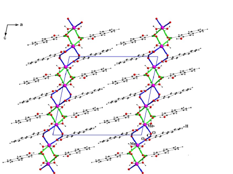
Figure 1: View along the $b$-axis of the metal-organic quantum magnet $\mathrm{Mn}[\mathrm{C}_{10}\mathrm{H}_{6}(\mathrm{OH})(\mathrm{COO})]_{2}\!\times\!2\mathrm{H}_{2}\mathrm{O}$. Bold lines show exchange paths $\mathrm{Mn}-\mathrm{O}-\mathrm{C}-\mathrm{O}-\mathrm{Mn}$. The unit cell, denoted by the parallelogram, contains four crystallographically equivalent $\mathrm{Mn}^{2+}$ ions.

These effects are of particular importance in low-dimensional magnets, e.g. $2\mathrm{D}$ layer structures with strong magnetic couplings within the layers and weak interactions between the layers. Such layer structures can be built up chemically from spin-bearing metal ions, which are connected by short bridges, being separated by organic fragments of considerable size, see Fig. 1. Motivated by these considerations we synthesized transition metal complexes of o-hydroxy-naphthoic acids. The crystal structure of $\mathrm{Mn}[\mathrm{C}_{10}\mathrm{H}_{6}(\mathrm{OH})(\mathrm{COO})]_{2}\!\times\!2\mathrm{H}_{2}\mathrm{O}$ (systematic name: manganese(II) 3-hydroxy-2-naphthoate dihydrate, Fig. 2) is of particular interest, because the $\mathrm{Mn}^{2+}$ ions form a distorted honeycomb lattice (Fig. 3). For the redetermination of the crystal structure, pale brown crystals were slowly grown by diffusion of an aqueous solution of $\mathrm{Na}[\mathrm{C}_{10}\mathrm{H}_{6}(\mathrm{OH})(\mathrm{COO})]$ into an aqueous $\mathrm{MnSO}_{4}$ solution with a buffer layer of water. The single crystal X-ray analysis confirmed the previously determined structureSchmidt04 with a higher precision. The compound crystallizes in the monoclinic space group $P2_{1}/c$ with the lattice parameters $a=17.191(4)\,\mathrm{\AA}$, $b=7.3448(10)\,\mathrm{\AA}$, $c=15.5279(17)\,\mathrm{\AA}$, $\beta=101.964(8)^{\circ}$, $V=1918.1(5)\,\mathrm{\AA}^{3}$.CCDC The unit cell contains four crystallographically equivalent $\mathrm{Mn}^{2+}$ ions.

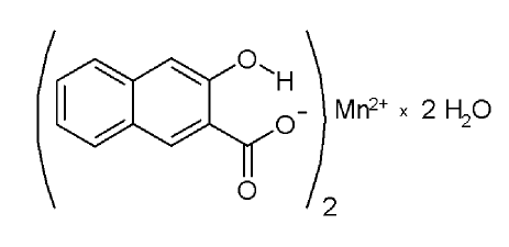
Figure 2: Chemical formula of $\mathrm{Mn}[\mathrm{C}_{10}\mathrm{H}_{6}(\mathrm{OH})(\mathrm{COO})]_{2}\!\times\!2\mathrm{H}_{2}\mathrm{O}$.

The coupling layer, parallel to the $(bc)$ plane, contains the $\mathrm{Mn}^{2+}$ ions, the $\mathrm{COO}^{-}$ and $\mathrm{OH}$ groups as well as water molecules. The isolating layer, having a thickness of about $12\,\mathrm{\AA}$ consists of the organic naphthalene moieties. These naphthalene moieties are only bound together by van der Waals contacts between C and H atoms. The relative weakness of these interactions is reflected by the morphology of the crystals: the crystals grow in ($b$) and ($c$) direction much faster than in ($a$) direction, thus forming thin plates parallel to the ($bc$) plane.

The magnetism is due to the $S=5/2$ manganese ions which form a distorted honeycomb pattern parallel to the ($bc$) planes. Neighboring ions are connected by carboxylic groups, which provide an $\mathrm{Mn}-\mathrm{O}-\mathrm{C}-\mathrm{O}-\mathrm{Mn}$ magnetic exchange path. There are two different exchange paths: the first path contains a single $\mathrm{O}-\mathrm{C}-\mathrm{O}$ unit, displayed in green in Fig. 3. In the second path (marked with blue color) the $\mathrm{Mn}^{2+}$ ions are connected by two $\mathrm{O}-\mathrm{C}-\mathrm{O}$ moieties simultaneously. The honeycomb layers are well separated from each other; the closest distances between $\mathrm{Mn}^{2+}$ ions of different layers are as large as $16.282\,\mathrm{\AA}$.

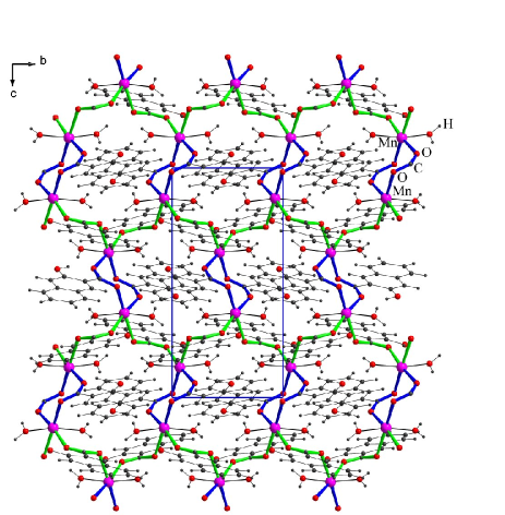
Figure 3: View on the $(bc)$ plane of the metal-organic quantum magnet $\mathrm{Mn}[\mathrm{C}_{10}\mathrm{H}_{6}(\mathrm{OH})(\mathrm{COO})]_{2}\!\times\!2\mathrm{H}_{2}\mathrm{O}$.

The structure in Fig. 3 suggests that the magnetic properties of the material can be modeled by a spin $S=5/2$ Heisenberg magnet on the distorted honeycomb lattice shown in Fig. 4. The exchange integrals $J_{\nu}=J({\bm{r}}_{i},{\bm{r}}_{i}+\bm{\delta}_{\nu})$, $\nu=1,2,3$, couple the spin at a given site ${\bm{r}}_{i}$ to its nearest neighbors at ${\bm{r}}_{i}+{\bm{\delta}}_{\nu}$. All exchange integrals $J_{\nu}$ turn out to be positive, and $\left|\bm{\delta}_{1}\right|=\left|\bm{\delta}_{3}\right|\equiv\delta_{1}=5.131(4)\,\mathrm{\AA}$ and $J_{1}=J_{3}$, due to the crystal symmetry. A closer look at the crystal structure in Fig. 3 and a comparison with the distorted honeycomb lattice in Fig. 4 reveals that $J_{2}$ acts along two exchange paths while $J_{1}$ results from a single exchange path. Therefore we expect $J_{2}$ to be roughly twice as large as $J_{1}$. Furthermore, the honeycomb lattice is bipartite, i.e., it can be divided into two sublattices, labeled A and B, such that the nearest neighbors of all sites belonging to sublattice A are located on sublattice B. Thus, for positive $J_{\nu}$ the system is not frustrated, and when quantum fluctuations are neglected the ground state shows classical antiferromagnetic Néel order. More generally, we expect long-range antiferromagnetic order to persist in the quantum mechanical ground state. Therefore, it should be possible to calculate the magnetic properties of the system within the usual spin-wave expansion, at least for temperature $T=0$. Note that the actual structure shown in Fig. 3 has an additional distortion in the $x$-direction, resulting in a primitive cell with doubled volume. Due to the low symmetry of the lattice the Dzyaloshinskii-Moriya interaction might play an important role. However, we expect the corresponding energy scale to be small in comparison with $J_{1}$ and $J_{2}$, so that in the first approximation we can neglect this effect. In the following we therefore always work with the magnetically equivalent Bravais lattice shown in Fig. 4.

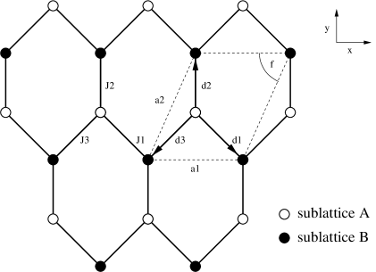
Figure 4: Distorted honeycomb lattice. The interactions between spins are displayed as solid lines. The underlying magnetic sublattice is a Bravais lattice and its primitive cell can be chosen to be the dashed parallelogram. The corresponding primitive vectors are ${\bm{a}}_{1}=a_{1}{\hat{\bm{e}}}_{x}$ and ${\bm{a}}_{2}=a_{2}\cos{\varphi}\,{\hat{\bm{e}}}_{x}+a_{2}\sin{\varphi}\,{\hat{\bm{e}}}_{y}$.

Measurements of the magnetization $M(H,T)$ in a magnetic field $H$ are performed at finite temperatures $T$, where long-range antiferromagnetic order is ruled out by the Hohenberg-Mermin-Wagner theorem.Hohenberg67 In this case the theoretical justification for the spin-wave expansion in two dimensions is more subtle. As long as there is long-range antiferromagnetic order at $T=0$, it is reasonable to expect that the low-energy and long-wavelength physics is still dominated by renormalized spin-waves. The magnetic properties of square lattice antiferromagnets in the absence of uniform external fields have been thoroughly investigated in a classical work by Chakravarty, Halperin, and Nelson. Chakravarty88 Less is known about the low-energy physics of two-dimensional quantum antiferromagnets subject to a uniform external magnetic field. The external field breaks the rotational symmetry of the Heisenberg antiferromagnet to O(2), similar to the effect of an XY anisotropy in the XXZ model.Fukumoto96 However, the classical ground states of the two models differ substantially: whereas the XXZ model has a collinear ground state, an uniform magnetic field in a Heisenberg antiferromagnet leads to a canted classical spin configuration shown in Fig. 5. The zero-temperature magnetization curve $M(H,0)$ of the square lattice antiferromagnet has been calculated a few years ago by Zhitomirsky and Nikuni Zhitomirsky98 within the spin-wave expansion. For finite temperatures, $M(H,T)$ has been extrapolated from numerical diagonalizations of finite clusters.Fabricius92 We are not aware of any analytical calculations in the literature of $M(H,T)$ for two-dimensional quantum Heisenberg antiferromagnets at $T>0$. In this work, we calculate $M(H,T)$ using a modified spin-wave approach Kollar03 which takes the absence of a spontaneous staggered magnetization at finite temperatures into account. Our theoretical results for the magnetization curves as well as for the zero-field susceptibility $\chi(T)$ show a satisfactory agreement with our measurements for the compound $\mathrm{Mn}[\mathrm{C}_{10}\mathrm{H}_{6}(\mathrm{OH})(\mathrm{COO})]_{2}\!\times\!2\mathrm{H}_{2}\mathrm{O}$.

The rest of the paper is organized as follows. In Sec. II we review the formalism of the spin-wave expansion for non-collinear spin configurations. In Sec. III this method is applied to an antiferromagnet on a bipartite lattice in the presence of a uniform magnetic field. Expressions for the magnetization, the staggered magnetization and the uniform susceptibility for the material of interest are obtained. We explain how a self-consistently determined staggered field is used to regularize divergencies at finite temperature. In Sec. IV we present results and compare with experimental measurements. Finally, in Sec. V we present our conclusion.

II Spin waves in non-collinear spin configurations

In the presence of a homogeneous magnetic field an antiferromagnet on a bipartite lattice has a non-collinear, canted spin configuration as shown in Fig. 5. We choose a coordinate system such that the uniform external field points along the $x$-axis, and the staggered magnetization is directed along the $z$-axis. The low temperature physics is dominated by spin-wave excitations. To obtain their spectrum we should quantize the spin-operators in a spatially-dependent (“co-moving”) coordinate system that matches for each site the axis defined by the expectation value $\langle\bm{S}_{i}\rangle$ of the spin operator.

Figure 5: Spin configuration $\langle\bm{S}_{i}\rangle$ in the classical ground state of a two-sublattice antiferromagnet . The dashed arrows represent a uniform magnetic field $B\hat{\bm{e}}_{x}$ in the $x$-direction and a staggered magnetic field $\zeta_{i}B_{s}\hat{\bm{e}}_{z}$ in the $z$-direction. The small solid arrows represent the vectors of a “co-moving” basis that matches the direction defined by the local magnetization $\langle\bm{S}_{i}\rangle$. Not shown are the basis vectors $\hat{\bm{e}}_{\mathrm{A}}^{1}=\hat{\bm{e}}_{\mathrm{B}}^{1}=\hat{\bm{e}}_{y}$ which point into the plane of the paper.

More generally, the problem of calculating the spin excitations of a Heisenberg magnet subject to an arbitrary inhomogeneous magnetic field ${\bm{B}}_{i}$ can be formulated and solved in a coordinate-free vector notation.Schuetz03 Consider the general Heisenberg hamiltonian

$$\hat{H}=\frac{1}{2}\sum_{i,j}J_{ij}{\bm{S}}_{i}\cdot{\bm{S}}_{j}-g\mu_{\text{B}}\sum_{i}{\bm{B}}_{i}\cdot{\bm{S}}_{i}\,,$$ (1)

where $J_{ij}=J(\bm{r}_{i},\bm{r}_{j})$ are some arbitrary exchange couplings, the sums are over all sites ${\bm{r}}_{i}$ of a $D$-dimensional lattice consisting of $N$ sites, and the ${\bm{S}}_{i}$ are spin-$S$ operators normalized such that ${\bm{S}}_{i}^{2}=S(S+1)$. The last term represents the Zeeman energy, where $g$ is the gyromagnetic factor and $\mu_{\mathrm{B}}$ is the Bohr magneton. We assume that the external magnetic field is sufficiently strong to induce permanent magnetic dipole moments ${\bm{m}}_{i}=g\mu_{\mathrm{B}}\langle{\bm{S}}_{i}\rangle$, where $\langle\ldots\rangle$ denotes the thermal equilibrium average. It is then convenient to decompose the spin operators as ${\bm{S}}_{i}=S^{\parallel}_{i}\hat{\bm{m}}_{i}+{\bm{S}}^{\bot}_{i}$, where ${\bm{S}}_{i}^{\bot}\cdot\hat{\bm{m}}_{i}=0$, and $\hat{\bm{m}}_{i}=\bm{m}_{i}/|{\bm{m}}_{i}|$ is a unit vector in the direction of $\bm{m}_{i}$. Substituting this decomposition into Eq. (1) we obtain $\hat{H}=\hat{H}^{\parallel}+\hat{H}^{\bot}+\hat{H}^{\prime}$, with

$$\hat{H}^{\parallel}\,\, = \frac{1}{2}\sum_{i,j}J_{ij}\hat{\bm{m}}_{i}\cdot\hat{\bm{m}}_{j}{{S}}_{i}^{\parallel}{{S}}_{j}^{\parallel}-\sum_{i}{\bm{h}}_{i}\cdot\hat{\bm{m}}_{i}{{S}}_{i}^{\parallel}\,,$$ (2)

$$\hat{H}^{\bot} = \frac{1}{2}\sum_{i,j}J_{ij}{\bm{S}}^{\bot}_{i}\cdot{\bm{S}}^{\bot}_{j}\,,$$ (3)

$$\hat{H}^{\prime}\,\, = -\sum_{i}{\bm{S}}^{\bot}_{i}\cdot\bigl{(}{\bm{h}}_{i}-\sum_{j}J_{ij}{{S}}_{j}^{\parallel}\hat{\bm{m}}_{j}\bigr{)}\,,$$ (4)

where ${\bm{h}}_{i}=g\mu_{\mathrm{B}}{\bm{B}}_{i}$. Note that $\hat{H}^{\prime}$ describes the coupling between the transverse and the longitudinal spin fluctuations. The classical ground state energy ${E}_{0}^{\rm cl}$ is obtained by replacing $S_{i}^{\parallel}\rightarrow S$ in Eq. (2) and by finding the configuration $\{\hat{\bm{m}}_{i}\}$ that minimizes the resulting classical hamiltonian

$$H^{\rm cl}=\frac{S^{2}}{2}\sum_{i,j}J_{ij}\hat{\bm{m}}_{i}\cdot\hat{\bm{m}}_{j}-S\sum_{i}{\bm{h}}_{i}\cdot\hat{\bm{m}}_{i}\;.$$ (5)

A necessary condition for an extremum of Eq. (5), taking into account the constraints $\hat{\bm{m}}_{i}^{2}=1$, is Schuetz03

$$\hat{\bm{m}}_{i}\times\Big{(}{\bm{h}}_{i}-S\sum_{j}J_{ij}\hat{\bm{m}}_{j}\Big{)}=0\,.$$ (6)

For given ${\bm{h}}_{i}$ and $J_{ij}$, this is a system of non-linear equations for the spin directions $\hat{\bm{m}}_{i}$ in the classical ground state. Using Eq. (6), the part $\hat{H}^{\prime}$ of the hamiltonian describing the coupling between transverse and longitudinal fluctuations can be written as

$$\hat{H}^{\prime}=-\sum_{i,j}J_{ij}({\bm{S}}_{i}^{\bot}\cdot\hat{\bm{m}}_{j})(S-S_{j}^{\parallel})\;.$$ (7)

Let us expand the transverse components of ${\bm{S}}^{\bot}_{i}$ in a spherical basis, ${\bm{S}}^{\bot}_{i}$ $=$ $\frac{1}{2}\sum_{p=\pm}S_{i}^{-p}{\bm{e}}^{p}_{i}$, with the spherical basis vectors ${\bm{e}}^{p}_{i}$ $=$ $\hat{\bm{e}}^{1}_{i}+ip\hat{\bm{e}}^{2}_{i}$, $p$ $=$ $\pm$, where $\left\{\hat{\bm{e}}_{i}^{1},\hat{\bm{e}}_{i}^{2},\hat{\bm{m}}_{i}\right\}$ is a local orthogonal triad of unit vectors. The transverse part of our spin hamiltonian can then be written as

$$\hat{H}^{\bot}=\frac{1}{8}\sum_{i,j}\sum_{p,p^{\prime}}J_{ij}({\bm{e}}^{p}_{i}\cdot{\bm{e}}^{p^{\prime}}_{j}){{S}}^{-p}_{i}{{S}}^{-p^{\prime}}_{j}\,.$$ (8)

The basis vectors $\hat{\bm{e}}_{i}^{1},\hat{\bm{e}}_{i}^{2}$ are not unique: any rotation around $\hat{\bm{m}}_{i}$ yields an equally acceptable transverse basis.

So far, no approximation has been made. To obtain the spin-wave spectrum, we expand the spin operators in terms of canonical boson operators $b_{i}$ as usual Dyson56 ; Maleev57 , $S^{\parallel}_{i}$ $=$ $S-b_{i}^{\dagger}b_{i}^{\phantom{\dagger}}$ and $S^{+}_{i}$ $=$ $(S^{-}_{i})^{\dagger}$ $=$ $\sqrt{2S}\,b_{i}^{\phantom{\dagger}}\,(1+O(S^{-1}))$. Within the linear spin-wave approximation the hamiltonian becomes $\hat{H}\approx E_{0}^{\rm cl}+\hat{H}_{2}$, where $E_{0}^{\rm cl}$ is the minimum of the classical hamiltonian $H^{\rm cl}$ in Eq. (5), and

$$\hat{H}_{2} = \frac{S}{4}\sum_{i,j}J_{ij}[(\bm{e}^{+}_{i}\cdot\bm{e}^{-}_{j})\;b_{i}^{\dagger}b_{j}+(\bm{e}^{-}_{i}\cdot\bm{e}^{+}_{j})\;b_{j}^{\dagger}b_{i}$$ (9)

$$\hskip 34.1433pt+(\bm{e}^{+}_{i}\cdot\bm{e}^{+}_{j})\;b_{i}^{\dagger}b_{j}^{\dagger}+(\bm{e}^{-}_{i}\cdot\bm{e}^{-}_{j})\;b_{j}b_{i}]$$

$$- \frac{S}{2}\sum_{i,j}J_{ij}({\hat{\bm{m}}}_{i}\cdot\hat{\bm{m}}_{j})[b^{\dagger}_{i}b_{i}+b^{\dagger}_{j}b_{j}]$$

$$+ \sum_{i}(\bm{h}_{i}\cdot\hat{\bm{m}}_{i})b^{\dagger}_{i}b_{i}\;.$$

Note that the contribution from $\hat{H}^{\prime}$ in Eq. (7) is of order $S^{1/2}$ and hence can be neglected within linear spin-wave theory. Eq. (9) together with Eqs. (5) and (6) completely determine the spin-wave spectrum of any Heisenberg magnet in an arbitrary inhomogeneous field.

III Spin waves in the distorted honeycomb lattice

III.1 Classical ground state

Let us apply the general formalism of the previous section to our bipartite lattice antiferromagnet in a uniform external magnetic field $B\hat{\bm{e}}_{x}$ along the $x$ axis. We denote by $\hat{\bm{e}}_{\alpha}$ fixed unit vectors in direction $\alpha=x,y,z$. For technical reasons we introduce an additional staggered magnetic field $\zeta_{i}B_{s}\hat{\bm{e}}_{z}$ in the $z$-direction, where $\zeta_{i}=1$ if ${\bm{r}}_{i}$ belongs to the A-sublattice and $\zeta_{i}=-1$ if ${\bm{r}}_{i}$ belongs to the B-sublattice. This auxiliary staggered field will be determined self-consistently in Sec. III.3 to insure a vanishing staggered magnetization at finite temperatures. The total magnetic field is thus

$$\bm{h}_{i}=g\mu_{\mathrm{B}}[B\hat{\bm{e}}_{x}+\zeta_{i}B_{s}\hat{\bm{e}}_{z}]\;.$$ (10)

The classical ground state configuration is then $\hat{\bm{m}}_{i}=\zeta_{i}\cos\theta\hat{\bm{e}}_{z}+\sin\theta\hat{\bm{e}}_{x}$, as shown in Fig. 5.

For convenience we introduce the notation $n_{0}=\cos\theta$ and $m_{0}=\sin\theta$. Physically, $m_{0}$ corresponds to the classical limit ($S\rightarrow\infty$) of the normalized uniform magnetization

$$m=\frac{1}{NS}\sum_{i}\langle\hat{\bm{e}}_{x}\cdot\bm{S}_{i}\rangle\;,$$ (11)

while $n_{0}$ corresponds to the $S\rightarrow\infty$ limit of the normalized staggered magnetization

$$n=\frac{1}{NS}\sum_{i}\zeta_{i}\langle\hat{\bm{e}}_{z}\cdot\bm{S}_{i}\rangle\;.$$ (12)

By symmetry, the uniform magnetization points into the $x$-direction, while the staggered magnetization points into the $z$-direction. The natural dimensionless measure for the strength of the fields is ${h}=\chi_{0}g\mu_{\mathrm{B}}B$ and ${h}_{s}=\chi_{0}g\mu_{\mathrm{B}}B_{s}$, where $\chi_{0}=(2\tilde{J}_{0}S)^{-1}$ is the classical uniform susceptibility. Here $\tilde{J}_{0}=\sum_{\nu}J_{\nu}$ is the ${\bm{k}}=0$ component of the Fourier transform of the exchange couplings

$$\tilde{J}_{\bm{k}}=\sum_{\nu}e^{-i{\bm{k}}\cdot\bm{\delta}_{\nu}}J_{\nu}\,.$$ (13)

For the special choice of the field $\bm{h}_{i}$ given in Eq. (10) our general Eq. (6) reduces to the simple relation

$${h}=m_{0}[1+{h}_{s}/n_{0}]\;,$$ (14)

which together with $n_{0}^{2}+m_{0}^{2}=1$ determines the classical Néel order parameter $n_{0}$ and the classical uniform magnetization $m_{0}$ as functions of the fields $h$ and $h_{s}$. Note that $\hat{\bm{m}}_{\mathrm{A}}\cdot\hat{\bm{m}}_{\mathrm{B}}=m_{0}^{2}-n_{0}^{2}$, and with the special transverse basis shown in Fig. 5

$$\bm{e}_{\mathrm{A}}^{p}\cdot\bm{e}_{\mathrm{B}}^{p^{\prime}} = 2[\delta_{p,p^{\prime}}n_{0}^{2}+\delta_{p,-p^{\prime}}m_{0}^{2}]\;,$$ (15)

$$\hat{\bm{m}}_{\mathrm{A}}\cdot{\bm{e}}_{\mathrm{B}}^{p} = 2ipn_{0}m_{0}=-\hat{\bm{m}}_{\mathrm{B}}\cdot{\bm{e}}_{\mathrm{A}}^{p}\;\;.$$ (16)

III.2 Spin-wave dispersion

To obtain the spin-wave dispersion, we must diagonalize $\hat{H}_{2}$ in Eq. (9) for the special ground-state spin configuration discussed above. Therefore, we first perform Fourier transformations separately on each sublattice,

$$b_{i} = \sqrt{\frac{2}{N}}\sum_{\bm{k}}e^{i{\bm{k}}\cdot{\bm{r}}_{i}}a_{\bm{k}}\;\;,\;\;\mbox{for $\bm{r}_{i}\in$ A }\;,$$ (17a)

$$b_{i} = \sqrt{\frac{2}{N}}\sum_{\bm{k}}e^{i{\bm{k}}\cdot{\bm{r}}_{i}}b_{\bm{k}}\;\;,\;\;\mbox{for $\bm{r}_{i}\in$ B }\;,$$ (17b)

where the wave-vector sums are over the reduced (magnetic) Brillouin zone of the honeycomb lattice shown in Fig. 6. With the above definitions we obtain

$$\hat{H}_{2} = \tilde{J}_{0}S\sum_{\bm{k}}\bigl{[}A(a^{\dagger}_{\bm{k}}a_{\bm{k}}+b^{\dagger}_{\bm{k}}b_{\bm{k}})+B_{\bm{k}}b_{-\bm{k}}a_{\bm{k}}+B_{\bm{k}}^{\ast}a^{\dagger}_{\bm{k}}b^{\dagger}_{-\bm{k}}$$ (18)

$$\hskip 42.67912pt+C_{\bm{k}}b^{\dagger}_{\bm{k}}a_{\bm{k}}+C_{\bm{k}}^{\ast}a^{\dagger}_{\bm{k}}b_{\bm{k}}\bigr{]}\;,$$

where $A=1+2{h}_{s}/n_{0}$, $B_{\bm{k}}=n_{0}^{2}\tilde{J}_{\bm{k}}/\tilde{J}_{0}$, and $C_{\bm{k}}=m_{0}^{2}\tilde{J}_{\bm{k}}/\tilde{J}_{0}$. On a honeycomb lattice $\tilde{J}_{\bm{k}}=|\tilde{J}_{\bf{k}}|e^{i\phi_{\bm{k}}}$ is complex, so that $B_{\bm{k}}=|B_{\bf{k}}|e^{i\phi_{\bm{k}}}$ and $C_{\bm{k}}=|C_{\bf{k}}|e^{i\phi_{\bm{k}}}$. Using $\phi_{-\bm{k}}=-\phi_{\bm{k}}$, it is easy to see that these phase factors can be removed from Eq. (18) via the gauge transformation $\tilde{a}_{\bm{k}}=e^{i\phi_{\bm{k}}}a_{\bm{k}}$. Introducing then new canonical boson operators

$$c_{\bm{k}\sigma}=\frac{1}{\sqrt{2}}\left[\tilde{a}_{\bm{k}}+\sigma b_{\bm{k}}\right]\;\;,\;\;\sigma=\pm 1\;,$$ (19)

the hamiltonian (18) assumes the block-diagonal form,

$$\hat{H}_{2} = \frac{\tilde{J}_{0}S}{2}\sum_{\bm{k}\sigma}\bigl{[}(A+\sigma|C_{\bm{k}}|)(c^{\dagger}_{\bm{k}\sigma}c_{\bm{k}\sigma}+c^{\dagger}_{-\bm{k}\sigma}c_{-\bm{k}\sigma})$$ (20)

$$\hskip 34.1433pt+\sigma|B_{\bm{k}}|(c^{\dagger}_{\bm{k}\sigma}c^{\dagger}_{-\bm{k}\sigma}+c_{\bm{k}\sigma}c_{-\bm{k}\sigma})\bigr{]}\;.$$

The diagonalization is completed by means of the Bogoliubov transformation,

$$\left(\begin{array}[]{c}c_{\bm{k}\sigma}\\ c^{\dagger}_{-\bm{k}\sigma}\end{array}\right)=\left(\begin{array}[]{cc}u_{\bm{k}\sigma}&-\sigma v_{\bm{k}\sigma}\\ -\sigma v_{\bm{k}\sigma}&u_{\bm{k}\sigma}\end{array}\right)\left(\begin{array}[]{c}d_{\bm{k}\sigma}\\ d^{\dagger}_{-\bm{k}\sigma}\end{array}\right)\;,$$ (21)

where

$$u_{\bm{k}\sigma} = \sqrt{\frac{A+\sigma|C_{\bm{k}}|+\epsilon_{\bm{k}\sigma}}{2\epsilon_{\bm{k}\sigma}}}\;,$$ (22a)

$$v_{\bm{k}\sigma} = \sqrt{\frac{A+\sigma|C_{\bm{k}}|-\epsilon_{\bm{k}\sigma}}{2\epsilon_{\bm{k}\sigma}}}\;,$$ (22b)

with the dimensionless energy dispersion

$$\epsilon_{\bm{k}\sigma}=\sqrt{(A+\sigma|C_{\bm{k}}|)^{2}-|B_{\bm{k}}|^{2}}\;.$$ (23)

Defining $\gamma_{\bm{k}}=\tilde{J}_{\bm{k}}/\tilde{J}_{0}$, we may write

$$\epsilon_{\bm{k}\sigma}=\Bigl{[}\bigl{(}1+\frac{2{h}_{s}}{n_{0}}+\sigma|\gamma_{\bm{k}}|\bigr{)}\bigl{(}1+\frac{2{h}_{s}}{n_{0}}-\sigma(n_{0}^{2}-m_{0}^{2})|\gamma_{\bm{k}}|\bigr{)}\Bigr{]}^{1/2}\;.$$ (24)

Figure 6: Reduced Brillouin zone of the distorted honeycomb lattice. The primitive vectors are ${\bm{b}}_{1}=\frac{2\pi}{a_{1}\sin{\varphi}}(\sin{\varphi}\,{\hat{\bm{e}}}_{x}-\cos{\varphi}\,{\hat{\bm{e}}}_{y})$ and ${\bm{b}}_{2}=\frac{2\pi}{a_{2}\sin{\varphi}}{\hat{\bm{e}}}_{y}$, where $a_{1}$, $a_{2}$ and the angle $\varphi$ are defined in Fig. 4.

In terms of the new operators $d_{\bm{k}\sigma}$ the quadratic spin wave hamiltonian $\hat{H}_{2}$ is diagonal,

$$\hat{H}_{2}=\tilde{J}_{0}S\sum_{\bm{k}\sigma}\left\{\epsilon_{\bm{k}\sigma}d^{\dagger}_{\bm{k}\sigma}d_{\bm{k}\sigma}+\frac{1}{2}\left[\epsilon_{\bm{k}\sigma}-(A+\sigma|C_{\bm{k}}|)\right]\right\}\;.$$ (25)

The low temperature properties of the magnet are determined by the long-wavelength behavior of the spin-wave dispersions, which follow from the expansion for small ${\bm{k}}$,

$$|\gamma_{\bm{k}}|\approx 1-\frac{1}{2}\sum_{\alpha\beta}k_{\alpha}A_{\alpha\beta}k_{\beta}\,,$$ (26)

where ${\bm{A}}$ is a matrix with elements

$$A_{\alpha\beta}=\sum_{\nu}\frac{J_{\nu}}{\tilde{J}_{0}}(\bm{\delta}_{\nu}\cdot\hat{\bm{e}}_{\alpha})(\bm{\delta}_{\nu}\cdot\hat{\bm{e}}_{\beta})-\sum_{\nu,\nu^{\prime}}\frac{J_{\nu}J_{\nu^{\prime}}}{\tilde{J}_{0}^{2}}(\bm{\delta}_{\nu}\cdot\hat{\bm{e}}_{\alpha})(\bm{\delta}_{\nu^{\prime}}\cdot\hat{\bm{e}}_{\beta})\,.$$ (27)

Since ${\bm{A}}$ is symmetric, an orthogonal basis can always be chosen such that ${\bm{A}}$ is diagonal, with eigenvalues $A_{\alpha}$. In this basis

$$|\gamma_{\bm{k}}|\approx 1-\frac{1}{2}\sum_{\alpha}A_{\alpha}k_{\alpha}^{2}\,.$$ (28)

The matrix ${\bm{A}}$ is positive, since

$$|\gamma_{\bm{k}}|\leq\sum_{\nu}\left|\frac{J_{\nu}}{\tilde{J}_{0}}\right|=1\,,$$ (29)

where the last equality assumes that all couplings have the same sign. We can thus define effective length scales $\ell_{\alpha}$ by setting $A_{\alpha}=\ell_{\alpha}^{2}$. For a $D$-dimensional hypercubic lattice with lattice spacing $a$ we have $\ell^{2}_{\alpha}={a^{2}}/{D}$. For our honeycomb lattice shown in Fig. 4 with $|\bm{\delta}_{1}|=|\bm{\delta}_{3}|$ and $J_{1}=J_{3}$ the eigenvectors of $\bm{A}$ are parallel to the $x$-axis and the $y$-axis, with corresponding eigenvalues $\ell_{x}^{2}=(J_{1}/2\tilde{J}_{0})a_{1}^{2}$ and $\ell_{y}^{2}=(2J_{1}J_{2}/\tilde{J}_{0}^{2})a_{2}^{2}\sin^{2}\varphi$. The spin-wave velocities $c_{\alpha}=\tilde{J}_{0}S\ell_{\alpha}$ along the two principal directions are thus

$$c_{x} = S\sqrt{\frac{J_{1}\tilde{J}_{0}}{2}}\,a_{1}\,,$$ (30)

$$c_{y} = S\sqrt{2J_{1}J_{2}}\,a_{2}\sin{\varphi}\,.$$ (31)

Note that for $J_{2}\rightarrow 0$ the velocity $c_{y}$ vanishes, so that the system becomes one-dimensional, as is obvious from Fig. 4. On the other hand, for $J_{1}\rightarrow 0$ both velocities vanish, because in this limit the system consists of decoupled dimers.

For ${h}_{s}=0$ only the mode $\epsilon_{\bm{k}-}$ is gapless for ${\bm{k}}\rightarrow 0$, while the mode $\epsilon_{\bm{k}+}$ has the gap $2m_{0}$. To give a more explicit form for the long-wavelength spin-wave dispersions, we further assume $h_{s}\ll n_{0}$. Then

$$\epsilon_{{\bm{k}}-} \approx n_{0}\left[\frac{4h_{s}}{n_{0}}+\sum_{\alpha}(\ell_{\alpha}k_{\alpha})^{2}\right]^{1/2}\,,$$ (32)

$$\epsilon_{{\bm{k}}+} \approx \Bigl{[}4m_{0}^{2}+\frac{4h_{s}}{n_{0}}(1+m_{0}^{2})$$ (33)

$$+(n_{0}^{2}-2m_{0}^{2})\sum_{\alpha}(\ell_{\alpha}k_{\alpha})^{2}\Bigr{]}^{1/2}\,.$$

For $n_{0}\to 0$ the expansion (32) is not appropriate any longer and for $h_{s}=0$ the dispersion $\epsilon_{{\bm{k}}-}$ becomes purely quadratic at $n_{0}=0$. Before this happens, there is a critical field $0<h^{*}<1$ at which the curvature of the dispersion $\epsilon_{{\bm{k}}-}$ changes sign. The positive curvature for $h>h^{*}$ results in an instability of magnons towards a spontaneous decay into two magnon states.Zhitomirsky99 Furthermore, if an anisotropic exchange is considered, the anisotropy gap $\Delta$ is strongly renormalized by magnon interactions.Maleyev00 ; Syromyatnikov01 As the influence of these instabilities on the thermodynamic properties is unclear at the moment, they will not be further considered in this work.

III.3 Uniform and staggered magnetization

We now calculate the leading spin-wave corrections to the normalized uniform- and the staggered magnetization as defined in Eqs. (11) and (12). A standard expansion in powers of $1/S$ gives

$$m = \frac{m_{0}^{2}}{{h}}\left[1+\frac{n{h}_{s}}{n_{0}^{2}}-\frac{F({h},{h}_{s})}{S}\right]\;,$$ (34)

$$n = \frac{1}{n_{0}}\left[1-m_{0}m-\frac{I({h},{h}_{s})}{S}\right]\;,$$ (35)

where

$$F({h},{h}_{s})=\frac{1}{N}\sum_{\bm{k}\sigma}\frac{n_{\bm{k}\sigma}+\frac{1}{2}}{\epsilon_{\bm{k}\sigma}}\sigma|\gamma_{\bm{k}}|\Bigl{(}1+\frac{2{h}_{s}}{n_{0}}+\sigma|\gamma_{\bm{k}}|\Bigr{)}\;,$$ (36)

and

$$I({h},{h}_{s})=-\frac{1}{2}+\frac{1}{N}\sum_{\bm{k}\sigma}\frac{n_{\bm{k}\sigma}+\frac{1}{2}}{\epsilon_{\bm{k}\sigma}}\Bigl{(}1+\frac{2{h}_{s}}{n_{0}}+\sigma m_{0}^{2}|\gamma_{\bm{k}}|\Bigr{)}\;.$$ (37)

Here $n_{\bm{k}\sigma}=[e^{\tilde{J}_{0}S\epsilon_{\bm{k}\sigma}/T}-1]^{-1}$ is the Bose function. The parameters $n_{0}$ and $m_{0}$ on the right-hand sides of Eqs. (34–37) are determined as functions of the fields $h$ and $h_{s}$ by Eq. (14) and $n_{0}^{2}+m_{0}^{2}=1$. Note that for $S\rightarrow\infty$ the solutions of Eqs. (34) and (35) correctly approach $n=n_{0}$ and $m=m_{0}$: in this limit Eq. (34) reduces to Eq. (14), while Eq. (35) simply becomes another way of writing $n_{0}^{2}+m_{0}^{2}=1$. In the thermodynamic limit, we transform Brillouin zone sums to integrals according to

$$\frac{2}{N}\sum_{\bm{k}}\stackrel{{\scriptstyle N\to\infty}}{{\longrightarrow}}V_{u}\int_{\text{BZ}}\frac{d^{2}k}{(2\pi)^{2}}\,,$$ (38)

where $V_{u}=a_{1}a_{2}\sin\varphi$ is the area of the magnetic unit cell in real space and the integral is over the reduced Brillouin zone shown in Fig. 6.

At $T=0$ and $h_{s}=0$ expressions similar to (34) and (35) have been discussed previously.Zhitomirsky98 Only $m(h)$ was given explicitly and a renormalization of the canting angle was found by considering spin-wave interactions. Yet, to a given order in $1/S$ it is easier to calculate $m$ and $n$ directly as derivatives of the free energy with respect to $h$ and $h_{s}$. Very recently, the renormalized canting angle was also used to analyze the behavior of $n(h)$ at $T=0$ for a more complicated geometry.Veillette05

At any finite temperature the integral $I(h,0)$ is infrared divergent in two dimensions, signaling the absence of long-range antiferromagnetic order, in accordance with the Hohenberg-Mermin-Wagner theorem.Hohenberg67 At first sight, it thus seems that the finite-temperature magnetization curve cannot be calculated within our spin-wave approach. Fortunately, there is a straightforward way to obtain an approximate expression for the magnetization even at finite $T$. The crucial observation is that if we set $n=0$ in Eqs. (34) and (35), these equations can be interpreted as a condition for the staggered field $h_{s}$ that is necessary to enforce a vanishing staggered magnetization. The solution $h_{s}=h_{s}(h)$ as a function of the uniform field $h$ is not a physical external staggered field, but an internal effective field that is generated by strong fluctuations. In fact, the field $h_{s}(h)$ is nothing but the Lagrange multiplier introduced in Takahashi’s modified spin-wave theory.Takahashi89 ; Kollar03 It is well known that the internal field is related to a finite correlation length $\xi$, as we will further discuss in Sec. IV.3. Numerically, we calculate the uniform magnetization $m(h,T)$ at finite temperature $T$ by adjusting $h_{s}$ for fixed external field $h$ such that the condition $n=0$ is fulfilled in Eqs. (34) and (35). Using this $h_{s}(h)$ in Eq. (34) then directly yields $m(h,T)$.

We must keep in mind that the staggered field $h_{s}$ does not respect the rotational symmetry of the original hamiltonian, which for $h=0$ corresponds to a global O(3) symmetry and for $h>0$ is reduced to a global O(2) symmetry around the axis of the uniform field. With the parametrization that explicitly breaks this symmetry, we should therefore only calculate rotationally invariant quantities.Kopietz97 Below, we will find a disagreement between a rotationally invariant evaluation of the zero-field uniform susceptibility and the slope of $\partial m/\partial h$ for $h\to 0$. We attribute this discrepancy to the fact that $\partial m/\partial h{|}_{h\to 0}$ does not respect the O(3) symmetry in this limit. Generally, we expect our approach for the finite temperature magnetization to be reasonable only for $h>h_{s}(h,T)$. In Sec. IV.3 we will see that $h_{s}$ is exponentially small at low temperatures, such that $h>h_{s}(h,T)$ is fulfilled even for very small external fields. The condition $h>h_{s}(h,T)$ then roughly gives a limit of validity of our approach in terms of the temperature as $T\lesssim 0.5\tilde{J}_{0}S$. The fact that the limits $T\to 0$ and $h\to 0$ do not commute in a modified spin-wave expansion was first noticed by Takahashi.Takahashi89

III.4 Uniform susceptibility

In order to calculate the rotationally invariant uniform zero-field susceptibility per spin

$$\chi=\frac{1}{TN}\sum_{i,j}\langle\bm{S}_{i}\cdot\bm{S}_{j}\rangle\,,$$ (39)

we set the uniform magnetic field $B=0$ in Eq.(10). In this case $m=m_{0}=0$ and $n_{0}=1$, so that we obtain a doubly degenerate mode in Eq. (24) with dispersion

$$\epsilon_{\bm{k}\sigma}=\epsilon_{\bm{k}}=\sqrt{(1+2h_{s})^{2}-|\gamma_{\bm{k}}|^{2}}\,,$$ (40)

and the expression for the staggered magnetization (35) reduces to

$$n=1+\frac{1}{2S}-\frac{2}{NS}\sum_{\bm{k}}\frac{n_{\bm{k}}+\frac{1}{2}}{\epsilon_{\bm{k}}}\left(1+2h_{s}\right)\,.$$ (41)

As explained in the previous section we use a self-consistently determined staggered field $h_{s}$ to enforce a vanishing order parameter $n=0$.

The susceptibility (39) can be written as

$$\chi=\frac{1}{T}\left\langle\bm{S}_{\bm{q},+}\cdot\bm{S}_{-\bm{q},+}\right\rangle_{\bm{q}=0}\,,$$ (42)

where we have defined the linear combinations ($\sigma=\pm$)

$$\bm{S}_{\bm{q},\sigma}=\frac{1}{\sqrt{2}}\left(\bm{S}_{\bm{q}}^{\mathrm{A}}+\sigma\bm{S}_{\bm{q}}^{\mathrm{B}}\right)$$ (43)

of the Fourier-transformed spin operators on each sublattice

$$\bm{S}_{\bm{q}}^{\mathrm{A}/\mathrm{B}}=\sqrt{\frac{2}{N}}\sum_{\bm{r}_{i}\in\mathrm{A}/\mathrm{B}}e^{-i\bm{q}\cdot\bm{r}_{i}}\,\bm{S}_{i}\,.$$ (44)

Next we decompose the susceptibility into a transverse and a longitudinal part

$$\chi=\chi^{+-}+\chi^{zz}\,,$$ (45)

where

$$\chi^{+-} = \frac{1}{2T}\left\langle S^{+}_{\bm{q},+}S^{-}_{-\bm{q},+}+S^{+}_{\bm{q},+}S^{-}_{-\bm{q},+}\right\rangle_{\bm{q}=0}\,,$$ (46)

$$\chi^{zz} = \frac{1}{T}\left\langle S^{z}_{\bm{q},+}S^{z}_{-\bm{q},+}\right\rangle_{\bm{q}=0}\,.$$ (47)

We map the spin operators (44) onto canonical boson operators via a Dyson-Maleev transformationDyson56 ; Maleev57 and evaluate the thermal expectation values of the noninteracting state using the Wick theorem. Then the transverse susceptibility (46) is proportional to the right hand side of Eq. (41), and thus vanishes if we require $n=0$. Therefore, in our approximation only the longitudinal part contributes to the rotationally invariant uniform susceptibility,

$$\chi=\frac{2}{TN}\sum_{\bm{k}}n_{\bm{k}}(n_{\bm{k}}+1)\,.$$ (48)

Apart from a different normalization, this result has been obtained previously in Takahashi’s approach.Takahashi89 We evaluate Eq. (48) numerically in the thermodynamic limit.

IV Results

IV.1 Zero temperature uniform and staggered magnetization

In Figs. 7 and 8 we show results for the uniform and staggered magnetization at zero temperature. In two spatial dimensions, there are no divergent contributions to the integrals in Eqs. (34) and (35), indicating true long range order. We can thus set $h_{s}=0$ and consequently $m_{0}=h$. As the deviations from the classical curves are rather small for $S=5/2$, we present the curves for the extreme quantum case $S=1/2$.

Figure 7: Normalized uniform magnetization $m(h)$ for $T=0$ and $h_{s}=0$. The solid line is the zero-temperature magnetization curve for the honeycomb lattice with $S=1/2$ and $J_{1}=J_{2}$. For comparison we also show the corresponding curve for a square lattice and exact results for a linear antiferromagnetic chain.Griffiths64 However, the $S=1/2$ chain is critical, so it is not surprising that it is poorly described by means of the spin-wave theory. Note that for $h_{s}=0$ the classical equation (14) is simply $m_{0}=h$.

The uniform magnetization shows a positive curvature for all $0\leq h<1$ and lies generally below the classical straight line.Zhitomirsky98 This tendency is stronger for the honeycomb lattice and is even more pronounced for anisotropic exchange couplings with $J_{1}\gg J_{2}$. The number of nearest neighbors $z=3$ for the honeycomb lattice is lower than for the square lattice ($z=4$), and in the limit $J_{2}\ll J_{1}$ the system is almost one-dimensional. The observed tendency thus simply corresponds to increased quantum fluctuations in low dimensions. Beyond the saturation field $h=1$ the ground state has full collinear ferromagnetic order. This state as well as single magnon excitations above it are easily shown to be exact eigenstates. As the single magnon states become gapless at exactly the classical value $h=1$, the saturation field is not changed by quantum fluctuations or magnon interactions. The limit $h\to 1$ is reached with infinite slope in $m(h)$. The leading behavior is given by

$$m=1+\frac{V_{u}}{4\ell_{x}\ell_{y}}\frac{\delta h}{\pi S}\ln\left(4\delta h\right)\,,$$ (49)

where $\delta h=1-h$. This logarithmic asymptotics was first discussed in the language of Bose condensation of magnons below the saturation fieldGluzman93 and was later found for the square lattice ($V_{u}/4\ell_{x}\ell_{y}$=1) within linear spin-wave theory.Zhitomirsky98 For our distorted honeycomb lattice, we have

$$\frac{V_{u}}{\ell_{x}\ell_{y}}=\sqrt{\frac{(2J_{1}+J_{2})^{3}}{J_{1}^{2}J_{2}}}\,,$$ (50)

which diverges for $J_{1}\to 0$ or $J_{2}\to 0$ and thus exemplifies the increasing deviations from the classical curve for strongly anisotropic exchange couplings.

Figure 8: Normalized staggered magnetization $n(h)$ at $T=0$ for honeycomb (solid line) and square lattice with $S=1/2$ (dotted line). The classical equation $n_{0}=\sqrt{1-h^{2}}$ is plotted for comparison. We also show the curves for the anisotropic cases $J_{1}/J_{2}=10,100$.

The staggered magnetization in Fig. 8 shows a non-monotonic dependence on the applied uniform field. For vanishing $h$ the staggered magnetization decreases as we lower the effective dimensionality. An external field apparently suppresses quantum fluctuations and $n(h)$ first increases with $h$ before it reaches a maximum and then vanishes for $h\to 1$ with infinite slope. The asymptotic behavior is given by

$$n=-\frac{V_{u}}{2\ell_{x}\ell_{y}}\frac{\sqrt{\delta h}}{\pi S}\ln\left(4\delta h\right)\,.$$ (51)

Interestingly, the quantum corrections to the staggered magnetization are positive close to the saturation field and the spin-wave result therefore intersects the classical curve. In a quasi one-dimensional situation ($J_{2}\ll J_{1}$), quantum fluctuations are strong and the leading order spin-wave theory, when pushed to the limit of validity, predicts a quantum disordered phase for small uniform fields.

IV.2 Finite temperature magnetization and susceptibility

Magnetic measurements were carried out on a single crystalline sample of $\mathrm{Mn}[\mathrm{C}_{10}\mathrm{H}_{6}(\mathrm{OH})(\mathrm{COO})]_{2}\!\times\!2\mathrm{H}_{2}\mathrm{O}$ with a mass of $m_{\mathrm{BONA}}=0.65\,\mathrm{mg}$ using a Quantum Design SQUID magnetometer MPMS-XL. Isothermal magnetization runs at temperatures between $2$ and $200\,\mathrm{K}$ and fields up to $5\,\mathrm{T}$ were performed as well as measurements of the susceptibility in the temperature range $2-300\,\mathrm{K}$ for a magnetic field of $0.05-2\,\mathrm{T}$.Schmidt04

Figure 9: Uniform magnetization $m(h)$ for the honeycomb lattice with $S=5/2$ and $J_{1}=J_{2}$ for two values of $T$.

In Fig. 9 we show theoretical magnetization curves $m(h)$ for the honeycomb lattice with $S=5/2$ and $J_{1}=J_{2}$ at different temperatures $T$. For $T\ll\tilde{J}_{0}S$ the magnetization is almost linear throughout the entire field range. At intermediate temperatures $m(h)$ has an S-like shape with a positive curvature at small fields $h$ that changes to a negative curvature with increasing $h$. Similar low-temperature behavior of the magnetization curve has been observed in a quantum Monte Carlo study of the two-dimensional Heisenberg antiferromagnet on a square lattice.Woodward02

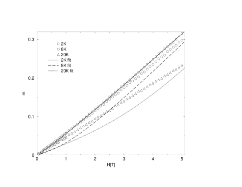
Figure 10: Magnetization $m(H)$ of $\mathrm{Mn}[\mathrm{C}_{10}\mathrm{H}_{6}(\mathrm{OH})(\mathrm{COO})]_{2}\!\times\!2\mathrm{H}_{2}\mathrm{O}$ up to field $H=5\,\mathrm{T}$. Experimental data are indicated by squares ($2\,\mathrm{K}$), circles ($8\,\mathrm{K}$) and triangles ($20\,\mathrm{K}$). Theoretical magnetization curves for honeycomb lattice with $S=5/2$ and $J_{2}=2J_{1}=1.95\,\mathrm{K}$ are denoted by lines.

It turns out that the magnetization as well as the susceptibility are not very sensitive to the ratio $J_{2}/J_{1}$ as long as $J_{1}$ and $J_{2}$ have the same order of magnitude. Thus, we cannot determine the precise value of $J_{2}/J_{1}$, but our fits are compatible with the assumption $J_{2}\approx 2J_{1}$.

In Fig. 10 we show experimental data and theoretical fits for the normalized uniform magnetization $m=M/(NS)$ at different temperatures. The magnetic field $H=2\tilde{J}_{0}Sh$ is given in Tesla. Surprisingly, all experimental curves are almost straight lines, whereas from Fig. 9 we would expect an upward bend of $m(h)$ at higher temperatures. Fits for $T=2\,\mathrm{K}$ and different ratios $J_{1}/J_{2}$ invariably give $\tilde{J}_{0}\approx 4\,\mathrm{K}$. Hence we assume $J_{2}=2J_{1}$ and fit the theoretical curve to the experimental data at $T=2\,\mathrm{K}$. Good agreement is achieved for $J_{2}=1.95\,\mathrm{K}$. For this value of the exchange couplings, we also plot theoretical magnetization curves at $T=8\,\mathrm{K}$ and $T=20\,\mathrm{K}$ in Fig. 10. These curves deviate significantly from the data, but one should be aware that $T=8K$ is already beyond the estimated limit of validity $T\lesssim 0.5\tilde{J}_{0}S$ of our theoretical approach.

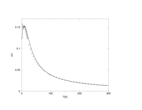
Figure 11: Susceptibility $\chi(T)$ of $\mathrm{Mn}[\mathrm{C}_{10}\mathrm{H}_{6}(\mathrm{OH})(\mathrm{COO})]_{2}\!\times\!2\mathrm{H}_{2}\mathrm{O}$. Circles are experimental data in a field of $2\,\mathrm{T}$. Theoretical fit for honeycomb lattice with $J_{2}=2J_{1}$ (solid line) gives $J_{2}=1.66K$.

In Fig. 11 the uniform susceptibility is plotted in the experimental units $\mathrm{cm^{3}/mol}$. When all exchange integrals have the same order of magnitude we expect a peak in the susceptibility for $T\approx\tilde{J}_{0}S$. Experimentally, the peak is at approximately $7\,\mathrm{K}$ so that we have $\tilde{J}_{0}\approx 3\,\mathrm{K}$, in accordance with the fits of the magnetization curves. For a more quantitative comparison we use the following procedure. First we substract the temperature-independent contribution from the experimental susceptibility in order to get the correct paramagnetic behavior at high temperatures. Then we fit the theoretical expression (48) with $J_{2}=2J_{1}$ to the full set of data points. Circles in Fig. 11 are experimental data and the solid line is a fit with $J_{2}=1.66\,\mathrm{K}$. The theoretical curve reproduces the behavior of the susceptibility very well and it especially gives a good estimate of the position and the form of the peak. Note that we experimentally observe an increase in the susceptibility below $T_{\ast}=3.0\pm 0.2\mathrm{K}$. This coincides with an anomaly in the specific heat. The careful reader will notice at this point that the estimated value of $T_{\ast}$ is larger than the temperature $T=2\,\mathrm{K}$ where we obtained the best fit of our calculated magnetization curve $m(H)$ to the experimental data shown in Fig. 10. Hence, at $T=2\,\mathrm{K}$ the system seems to have some kind of long range magnetic order, which we have ignored in our calculation. However, the precise nature of the order and the mechanism responsible for the ordering are not known at this point. The fact that a strictly 2D model can reasonably well explain the magnetization curve at $T=2\,\mathrm{K}$ imposes some constraint on possible ordering mechanisms. We suspect that dipole-dipole interactions play an important role in this temperature range, because the long-range nature of the dipole-dipole interaction can give rise to spontaneous antiferromagnetic order even in 2D.Pich93 This point deserves further attention, both theoretically and experimentally.

IV.3 Staggered correlation length in a magnetic field

The energy gap appearing in Eq. (32) can be related to the staggered correlation length $\xi$, as discussed by Takahashi.Takahashi89 Assuming for simplicity $|\bm{\delta}_{\nu}|=a$, we may identify

$$\left(\frac{a}{2\xi}\right)^{2}=\Delta^{2}=\frac{4h_{s}}{n_{0}}\,.$$ (52)

In the absence of a uniform field the low temperature behavior of $\xi$ has been thoroughly studied by Chakravarty, Halperin and Nelson.Chakravarty88 Surprisingly, the effect of a uniform field $h$ on $\xi$ has so far not been investigated. We now analyze the asymptotic behavior of $\xi$ at low temperatures. In two spatial dimensions, the limit $T\to 0$ also implies $h_{s}\to 0$. Our self-consistency equations (34) and (35) can then be solved analytically by isolating divergent contributions to the integrals $I(h,h_{s})$ and $F(h,h_{s})$ originating from gapless modes in the spin-wave spectrum. In the regular part of the integral, the limit $T\to 0$ and $h_{s}\to 0$ can be taken. For the leading behavior at small uniform fields $h\ll 1$ only the singular part of $I(h,h_{s})$ contributes, and we obtain the self-consistency condition

$$0=n(0)-\frac{I^{\text{sing}}(h,h_{s})}{S}\,.$$ (53)

Here, $I^{\text{sing}}(h,h_{s})$ is the part of the integral $I(h,h_{s})$ that diverges for vanishing gaps in the spin-wave dispersions, and $n(0)=n(h=0,h_{s}=0,T=0)$. For $h\ll 1$, we obtain

$$I^{\text{sing}}(h,h_{s}) = \frac{T}{\tilde{J}_{0}S}\frac{V_{u}}{2}\sum_{\sigma}\int\frac{d^{2}k}{(2\pi)^{2}}\frac{1}{\epsilon_{{\bm{k}}\sigma}^{2}}$$ (54)

$$\approx -\frac{T}{\tilde{J}_{0}S}\frac{V_{u}}{8\pi\ell_{x}\ell_{y}}\Bigg{[}\ln\left(\frac{4h_{s}}{n_{0}}\right)$$

$$+\ln\left(4h^{2}+\frac{4h_{s}}{n_{0}}\right)\Bigg{]}\,,$$

to leading logarithmic order. From Eqs. (52) and (53) we then obtain the following result for the self-consistent energy gap in a small uniform magnetic field

$$\Delta^{2}(h)=\left(\frac{a}{2\xi(h)}\right)^{2}=\sqrt{\Delta_{0}^{4}+\frac{(2h)^{4}}{4}}-\frac{(2h)^{2}}{2}\,,$$ (55)

where $\Delta_{0}=a/2\xi(0)$ is the gap for vanishing uniform field and the temperature dependence of the zero-field staggered correlation length is given by

$$\frac{\xi(0)}{a}\propto\exp\left(\frac{2\pi\tilde{J}_{0}S^{2}n(0)}{T}\frac{\ell_{x}\ell_{y}}{V_{u}}\right)\,.$$ (56)

For a square lattice this yields with $\tilde{J}_{0}=4J$ and $\ell_{x}\ell_{y}/V_{u}=1/4$

$$\frac{\xi(0)}{a}\propto\exp\left(\frac{2\pi JS^{2}n(0)}{T}\right)\,,$$ (57)

which is identical to Takahashi’s result (see Eq. (27a) in Ref. Takahashi89, ), except that we do not include a spin-wave velocity renormalization in our approach. To obtain this renormalization, the spin-wave interaction would have to be treated on the mean-field level in a fully self-consistent way.

The field dependence of the correlation length for fixed temperature is given by Eq. (55). For $h\ll\Delta_{0}(T)$, we have

$$\xi(h)=\xi(0)\left[1+\frac{1}{2}\left(\frac{h}{\Delta_{0}}\right)^{2}\right]\,,$$ (58)

whereas for $h\gg\Delta_{0}(T)$, we obtain

$$\frac{\xi(h)}{a}=4h\,\left(\frac{\xi(0)}{a}\right)^{2}\,.$$ (59)

From Eq. (55) it is clear that $\xi(h)>\xi(0)$. Thus, the correlation length is increased by a small uniform field due to reduced quantum fluctuations.

The temperature dependence of the correlation length for fixed uniform field $h$ can also be extracted from Eq. (55). As long as $\Delta_{0}(T)\gg 2h$, this temperature dependence is still given by Eq. (56). When the temperature is further reduced, Eq. (55) predicts a crossover at $\Delta_{0}(T)\approx 2h$ to the following temperature-dependent correlation length

$$\frac{\xi(h)}{a}\propto\exp\left(\frac{4\pi\tilde{J}_{0}S^{2}n(0)}{T}\frac{\ell_{x}\ell_{y}}{V_{u}}\right)\,.$$ (60)

The additional factor of two in the exponent as compared to Eq. (56) is due to the fact that at very low temperatures the spin-wave mode $\epsilon_{{\bm{k}}-}$ yields a singular contribution, whereas the mode $\epsilon_{{\bm{k}}+}$ has a gap $~{}2h$ which is fixed by the external field. In contrast, for $h=0$ both modes contribute equally, leading to Eq. (56).

The analysis in this section has been carried out for $h\ll 1$. For larger fields, there are field dependent prefactors of the first logarithm in Eq. (54) leading to a field dependent renormalization factor $Z_{h}$ in the exponent of Eq. (60). The field dependence of the correlation length at fixed temperature is then no longer determined by the singular contributions to the integrals and cannot be extracted from the simple analysis presented here. Close to the critical field at $h=1$ the nature of the divergences changes, since the dispersion of the $\sigma=-$ mode becomes quadratic. As our mean-field calculation is not suitable to describe the true critical behavior in two dimensions, we do not discuss this limit in more detail.

Our approach can also describe a quasi one-dimensional anisotropic system, where the exchange coupling between chains is very weak. The dispersion is then almost flat in the transverse direction. The integrals will be quasi one-dimensional as long as the maximum variation of the dispersion in the transverse direction is smaller than the self-consistent gap $4h_{s}/n_{0}$. In this intermediate temperature regime the staggered correlation length behaves as if the system were one-dimensional. At even lower temperatures there will be a crossover to the true asymptotic two-dimensional behavior. A rough estimate for the position of the crossover is ${a}/{\xi}\propto{\ell_{\bot}}/{a}$ where $\ell^{2}_{\bot}$ is the eigenvalue of the matrix $\bm{A}$ defined in Eq. (27) associated with the eigenvector perpendicular to the chain direction.

V Conclusion

In summary, we have investigated the magnetic properties of the new metal-organic quantum magnet $\mathrm{Mn}[\mathrm{C}_{10}\mathrm{H}_{6}(\mathrm{OH})(\mathrm{COO})]_{2}\!\times\!2\mathrm{H}_{2}\mathrm{O}$. Its layered structure contains two-dimensional arrangements of $\mathrm{Mn}^{2+}$ ions that suggest a spin $S=5/2$ Heisenberg model on a distorted honeycomb lattice as a minimal model. In order to explain measurements of the magnetization $M(H,T)$ and the susceptibility $\chi(T)$, we develop a variant of modified spin-wave theory, which can be used to describe finite temperature properties of two-dimensional magnets in a uniform external magnetic field. A fit of the theoretical results to the experimental curves shows a satisfactory agreement for the magnetization at low temperatures where we expect our theoretical approach to be valid. The magnetic susceptibility is very well described down to temperatures of $T\gtrsim T_{\ast}\approx 3\mathrm{K}$. Both quantities are consistently fitted by one parameter $J_{2}=2J_{1}$ to give the exchange coupling $J_{2}\approx 1.8\,\mathrm{K}$. For temperatures below $T_{\ast}$ the uniform susceptibility shows again an upturn, which together with an anomaly in the specific heat is most likely due to some ordering transition. Possible mechanisms for this transition are dipole-dipole interactions or couplings between the layers, which should be included in more refined theoretical models. From the experimental point of view nuclear magnetic resonance or neutron scattering measurements could provide a more detailed insight into the nature of the magnetic interactions.

This work was supported by the DFG via Forschergruppe FOR 412. We thank M. Kulić for interesting discussions and especially for pointing out the possible importance of dipole-dipole interactions.

References

- (1) For a collection of recent reviews see U. Schollwöck, J. Richter, D. J. J. Farnell, and R. F. Bishop (Eds.), Quantum Magnetism, (Springer, Berlin Heidelberg, 2004).
- (2) M. U. Schmidt, E. Alig, L. Fink, M. Bolte, R. Panisch, V. Pashchenko, B. Wolf, and M. Lang, Acta. Cryst. C 61, m361 (2005).
- (3) Details of the crystal structure determination are available from the Cambridge Crystallographic Data Centre, http://www.ccdc.cam.ac.uk/products/csd/request/ quoting the reference number CSD-269503.
- (4) P. C. Hohenberg, Phys. Rev. 158, 383 (1967); N. D. Mermin and H. Wagner, Phys. Rev. Lett. 17, 1133 (1966).
- (5) S. Chakravarty, B. I. Halperin, and D. R. Nelson, Phys. Rev. B 39, 2344 (1989).
- (6) Y. Fukumoto, J. Phys. Soc. Jpn. 65, 569 (1996);
- (7) M. E. Zhitomirsky and T. Nikuni, Phys. Rev. B 57, 5013 (1998).
- (8) K. Fabricius, M. Karbach, U. Löw, and K.-H. Mütter, Phys. Rev. B 45, 5315 (1992).
- (9) M. Kollar, I. Spremo, and P. Kopietz, Phys. Rev. B 67, 104427 (2003).
- (10) F. Schütz, M. Kollar, and P. Kopietz, Phys. Rev. Lett. 91, 017205 (2003); Phys. Rev. B 69, 035313 (2004).
- (11) F. J. Dyson, Phys. Rev. 102, 1217 and 1230 (1956);
- (12) S. V. Maleev, Zh. Eksp. Theor. Fiz. 30, 1010 (1957) [Sov. Phys. JETP 64, 654 (1958)].
- (13) M. E. Zhitomirsky and A. L. Chernyshev, Phys. Rev. Lett. 82, 4536 (1999).
- (14) S. V. Maleyev, Phys. Rev. Lett. 85, 3281 (2000).
- (15) A. V. Syromyatnikov and S. V. Maleyev, Phys. Rev. B 65, 12401 (2001).
- (16) M. Y. Veillette, J. T. Chalker, and R. Coldea, Phys. Rev. B 71, 214426 (2005).
- (17) M. Takahashi, Phys. Rev. B 40, 2494 (1989).
- (18) P. Kopietz and S. Chakravarty, Phys. Rev. B 56, 3338 (1997).
- (19) R. B. Griffiths, Phys. Rev. 133, A768 (1964)
- (20) S. Gluzman, Z. Phys. B 90, 313 (1993).
- (21) F. M. Woodward, A. S. Albrecht, C. M. Wynn, C. P. Landee, and M. M. Turnbull, Phys. Rev. B 65, 144412 (2002).
- (22) C. Pich and F. Schwabl , Phys. Rev. B 47, 7957 (1993).