Renormalization-group approach to superconductivity: from weak to strong electron-phonon coupling

Abstract

We present the numerical solution of the renormalization group (RG) equations derived in Ref.Tsai, , for the problem of superconductivity in the presence of both electron-electron and electron-phonon coupling at zero temperature. We study the instability of a Fermi liquid to a superconductor and the RG flow of the couplings in presence of retardation effects and the crossover from weak to strong coupling. We show that our numerical results provide an ansatz for the analytic solution of the problem in the asymptotic limits of weak and strong coupling.

The renormalization-group approach to interacting fermions in more than one spatial dimension shankar has been extensively applied to the study of instabilities of the Fermi liquid state, and has become a major tool in the study of correlated electron systems. Nevertheless, even for weak electron-electron interactions, the picture is far from being complete, since electrons in solids also interact with bosonic modes such as phonons. Therefore, the development of an RG scheme Tsai that includes both electron-electron and electron-phonon interactions on an equal footing is an important advance. Experimental evidence show that in many strongly correlated systems, such as high-temperature superconductors and organic charge transfer salts, both electron interactions and phonons seem to play an important roleshen ; organics ; mgb2 ; millis ; c60 .

The renormalization-group approach to interacting fermions coupled to phonons was presented in Ref. [Tsai, ]. This approach takes retardation effects and the presence of multiple energy scales fully into account. For a circular Fermi surface, the RG equations predict the onset of the superconducting instability in agreement withe Eliashberg’s superconducting theory eliashberg . A large-$N$ analysis, where $N\approx E_{F}/\Lambda$ is the number of patches in the Fermi surface ($E_{F}$ is the Fermi energy and $\Lambda$ is the size of the patch), shows that in this case Eliashberg theory is asymptotically exact and Migdal’s theorem migdal emerges as a consequence of the $1/N$ expansion. Here we present a numerical solution of the RG equations at $T=0$, showing how the couplings, which are functions of frequencies, flow with the RG procedure. In the limits of weak and strong phonon coupling, simple analytical expressions are extracted on the basis of the numerical solution.

For completeness, in Sec. I the RG equations for the self-energy and interaction couplings are derived. In Sec. II we present the numerical results, and the analytical expressions associated with the asymptotic limits. Sec. III contains the concluding remarks.

I Derivation of the RG equations

The action that describes electron-electron and electron-phonon interactions can be written as $S(\psi,\phi)=S_{e}(\psi)+S_{ph}(\phi)+S_{e-ph}(\psi,\phi)+S_{e-e}(\psi)$, where $\phi$ are bosonic fields, $\psi$ are fermionic (Grassman) fields (we use units such that $\hbar=1=k_{B}$),

$$S_{e}=\int_{\omega{\bf k}\sigma}\psi^{\dagger}_{k\sigma}(i\omega-\epsilon_{{\bf k}})\psi_{k\sigma}\,,$$ (1)

is the free electron action, $\epsilon_{{\bf k}}$ is the electron dispersion as a function of momentum ${\bf k}$, and

$$S_{ph}=\int_{\Omega{\bf q}}\phi^{\dagger}_{q}(i\Omega-w_{{\bf q}})\phi_{q}\,,$$ (2)

is the free phonon action where $w_{{\bf q}}$ is the phonon dispersion ($\sigma=\uparrow,\downarrow$ is the electron spin, $k=\{\omega,{\bf k}\}$ and $q=\{\Omega,{\bf q}\}$, where $\omega,\Omega$ are fermionic and bosonic Matsubara frequencies, respectively, and ${\bf k},{\bf q}$ are the momenta). The electron-phonon interaction can be written as:

$$S_{e-ph}=\int_{\omega{\bf k}\sigma}\int_{\Omega{\bf q}}g(q)\psi^{\dagger}_{k+q\sigma}\psi_{k\sigma}(\phi_{q}+\phi^{\dagger}_{-q})\,,$$ (3)

where $g(q)$ is the electron-phonon coupling constant. The electron-electron interactions have the form:

$$S_{e-e}=\frac{1}{2}\prod_{i=1}^{3}\int_{\omega_{i}{\bf k}_{i}\sigma\sigma^{\prime}}u(k_{4},k_{3},k_{2},k_{1})\psi^{\dagger}_{k_{4}\sigma}\psi_{k_{2}\sigma}\psi^{\dagger}_{k_{3}\sigma^{\prime}}\psi_{k_{1}\sigma^{\prime}}\,,$$ (4)

where $u(\{k_{i}\})$ is a general spin-independent electron-electron coupling which depends on the momenta and frequencies of the electrons, and $k_{4}=k_{1}+k_{2}-k_{3}$ due to momentum conservation.

Since the bosonic action is quadratic in the boson fields, they can be integrated out exactly, leading to an effective electron-electron problem with retarded interactions:

$$\tilde{u}(k_{4},k_{3},k_{2},k_{1})=u(k_{4},k_{3},k_{2},k_{1})-2g(k_{1},k_{3})g(k_{2},k_{4})D(k_{1}-k_{3})\,,$$ (5)

where

$$D(q)=\omega_{{\bf q}}/(\omega^{2}+\omega_{{\bf q}}^{2})$$ (6)

is the phonon propagator. Here we consider the case of a circular Fermi surface and anisotropic Einstein phonons, with $g(k,k^{\prime})=g_{0}$ and $\omega_{{\bf q}}=\omega_{E}$. In what follows, it is also convenient to define the dimensionless electron-phonon coupling constant

$$\lambda=2N(0)g_{0}^{2}/\omega_{E}\,.$$ (7)

In the Kadanoff-Wilson approach to RG the flow equations are obtained by computing the corrections to the couplings of the theory as the energy modes in a energy shell between $\Lambda$ and $\Lambda+d\Lambda$ are integrated out. The momenta, frequencies, and fields are then rescaled in such a way that the quadratic terms remain unchanged. This second step presents a difficulty in the electron-phonon problem. The momenta of the electrons scale differently in the directions parallel and perpendicular to the Fermi surface, while the momenta of the phonons scale isotropically. In our RG treatment of the electron-phonon problem Tsai , we use the quantum field theory version of the RG, with no rescaling. In this approach, corrections to the vertices of the model are written in term of running, i. e. cut-off–dependent, coupling functions. The RG flow equations for these running couplings are then obtained by imposing that the vertices are cut-off independent.

We start with the two-point vertex, which at one loop is given by Tsai

$$\Gamma^{(2)}(\Sigma(\omega,{\mathbf{k}}))=\Sigma_{\ell}(\omega,{\mathbf{k}})-\int_{-\infty}^{\infty}\frac{d\Omega}{2\pi}\int_{(\Lambda)}\frac{d^{2}{\mathbf{k}}^{\prime}}{(2\pi)^{2}}\frac{e^{i\Omega 0_{+}}}{i\Omega-\epsilon_{\mathbf{k}^{\prime}}-\Sigma_{\ell}(\Omega,{\mathbf{k}}^{\prime})}\tilde{u}(k,k^{\prime},k,k^{\prime})$$ (8)

where $k=(\omega,{\mathbf{k}})$ and $k^{\prime}=(\Omega,{\mathbf{k}}^{\prime})$, and $\Sigma_{\ell}(\omega,{\mathbf{k}})$ is the electronic self-energy which now flows under the RG, and the RG parameter $\ell=\log(\Lambda_{0}/\Lambda)$, so that $d\ell=-d\Lambda/\Lambda$. The RG equation for the electron self-energy is obtained by imposing the condition of renormalizability of the theory, that is,

$$\frac{d\Gamma^{(2)}}{d\ell}=0\,,$$ (9)

where $\ell=\log(\Lambda_{0}/\Lambda)$ and $d\ell=-d\Lambda/\Lambda$.

Notice that the interaction that appears in Eq. (8), $\tilde{u}(k,k^{\prime},k,k^{\prime})$, only describes the forward scattering channel ($k_{4}=k_{1}=k$, $k_{3}=k_{2}=k^{\prime}$) which, in the large $N$ limit, does not flow under RG Tsai . Therefore, it can be substituted by its unrenormalized value given by Eq. (5). The electron-electron part of the interaction, $u(k,k^{\prime},k,k^{\prime})=u_{0}$ contributes only to the real part of the self-energy and gives a shift in the chemical potential that can be reabsorded into the definition of the chemical potential shankar . The electron-phonon part for $\omega>0$, leads to the following RG equation for the imaginary part of the self-energy, $\Sigma^{{}^{\prime\prime}}(\omega)$:

$$\frac{\partial}{\partial\ell}\Sigma^{{}^{\prime\prime}}_{\ell}(\omega)=-\int_{-\infty}^{+\infty}\frac{d\Omega}{\pi}\lambda\omega_{E}D(\Omega-\omega)\frac{\Lambda_{\ell}(\Omega-\Sigma^{{}^{\prime\prime}}_{\ell}(\Omega))}{(\Omega-\Sigma^{{}^{\prime\prime}}_{\ell}(\Omega))^{2}+\Lambda_{\ell}^{2}}\ \ ,$$ (10)

where $\Lambda_{\ell}=\Lambda_{0}e^{-\ell}$ (where $\Lambda_{0}<E_{F}$ is the cut-off in the beginning of the RG flow and it is assumed to be much larger than the other energy scales in the problem). There is no dependence of $\Sigma^{{}^{\prime\prime}}_{\ell}$ on the direction of the momentum ${\mathbf{k}}$ because we are considering the case of isotropic Fermi surface, and the dependence on the magnitude of ${\mathbf{k}}$ is irrelevant shankar . It is convenient to write $\Sigma^{"}(\omega)=[1-Z(\omega)]\omega$, and the solution of Eq. (10) becomes:

$$Z_{\ell}(\omega)=1+\frac{1}{\omega}\int_{-\infty}^{+\infty}\frac{d\Omega}{2}\lambda\omega_{E}D(\Omega-\omega)\Omega F_{\ell}(\Omega)$$ (11)

where

$$F_{\ell}(\omega)=\frac{2}{\pi}\int_{W_{\ell}(\omega)}^{\infty}\frac{dW^{\prime}}{\left(Z_{W^{\prime}}(\omega)/Z_{W}(\omega)\right)^{2}\omega^{2}+W^{\prime 2}}\ \ ,$$ (12)

where we have introduce $W_{\ell}(\omega)=\Lambda_{\ell}/Z_{\ell}(\omega)$ is the new renormalized cut-off running scale. The dependence of $Z_{W}(\omega)$ on $W$ is weak (see below) and therefore we can write $Z_{W}(\omega)\approx Z_{W^{\prime}}(\omega)$. In this case (12) can be solved at once:

$$F_{\ell}(\omega)\approx\frac{1}{|\omega|}\left[1-\frac{2}{\pi}\tan^{-1}\left(\frac{W_{\ell}(\omega)}{|\omega|}\right)\right]\,.$$ (13)

In what follows we will be only interested in the low frequency behavior, in which case $W_{\ell}(\omega)$ can be safely replaced by $W_{\ell}(\omega=0)$, the expression for $Z_{\ell}(\omega)$ can be easily evaluated from (11) to give

$$Z_{\ell}(\omega)=1-\lambda\frac{\omega_{E}}{\omega}\left[\tan^{-1}\left(\frac{W_{\ell}+\omega_{E}}{|\omega|}\right)-\frac{\pi}{2}\right]\,.$$ (14)

Notice that indeed the dependence of $Z_{W}$ on $W$ is weak, as assumed previously. In the static limit, $\omega\to 0$, one obtains

$$Z_{\ell}(0)=1+\lambda\omega_{E}/(W_{\ell}+\omega_{E})\,.$$ (15)

So far we have considered the renormalization of the self-energy. The renormalization of the interaction in the Cooper channel ($k_{4}=-k_{3}$ and $k_{2}=-k_{1}$) can be obtained in a completely analogous way. Since we are considering the case of a circular Fermi surface, we can focus on the $s$-wave component of the BCS interaction $\tilde{v}(\omega_{1},\omega_{3})\!=\!N(0)\int d\theta_{1}/2\pi\int d\theta_{3}/2\pi\tilde{u}(-k_{3},k_{3},-k_{1},k_{1})$. The RG equation for this interaction can be shown to be Tsai :

$$\frac{\partial}{\partial\ell}\tilde{v}(\omega_{1},\omega_{2},\ell)=-\int_{-\infty}^{+\infty}\frac{d\omega}{\pi}\frac{\Lambda_{\ell}}{[\omega-\Sigma_{\ell}^{{}^{\prime\prime}}(\omega)]^{2}+\Lambda_{\ell}^{2}}\tilde{v}(\omega_{1},\omega,\ell)\,\tilde{v}(\omega,\omega_{2},\ell)\,,$$ (16)

where the initial condition for the flow is given by $\tilde{v}(\omega_{1},\omega_{3},\ell=0)=u_{0}-\lambda\omega_{E}D(\omega_{1}-\omega_{3})$. Equation (16) can be written in matrix equation as:

$$\frac{\partial{\bf U}}{\partial\ell}=-{\bf U}\cdot{\bf M}\cdot{\bf U}$$ (17)

where

$$U_{ij}(\ell) = \tilde{v}(\omega_{i},\omega_{j},\ell)$$ (18)

$$M_{ij}(\ell) = \Lambda_{\ell}\delta_{ij}/[(\omega_{i}-\Sigma^{{}^{\prime\prime}}_{\ell}(\omega_{i}))^{2}+\Lambda_{\ell}^{2}]\,.$$ (19)

Formally, we can rewrite (17) as

$$\frac{\partial{\bf U}^{-1}}{\partial\ell}={\bf M}$$ (20)

since ${\bf U}^{-1}\partial_{\ell}{\bf U}{\bf U}^{-1}=-\partial_{\ell}{\bf U}^{-1}$. The solution of (20) reads:

$${\bf U}^{-1}(\ell)={\bf U}^{-1}(0)+{\bf P}(\ell)$$ (21)

where

$${\bf P}(\ell)=\int_{0}^{\ell}d\ell^{\prime}{\bf M}(\ell^{\prime})\,,$$ (22)

which can inverted to give:

$${\bf U}(\ell)=[{\bf 1}+{\bf U}(0)\cdot{\bf P}(\ell)]^{-1}\cdot{\bf U}(0)\,.$$ (23)

Eq.(23) allows the study of instabilities of the Fermi liquid state towards superconducting instabilities. The instabilities occur when one of the couplings diverges under the RG flow. These instabilities happen at some finite energy (or temperature) scale $\ell_{c}$ at which one of the eigenvalues of the coupling matrix ${\bf U}(\ell_{c})$ diverges at $\ell=\ell_{c}$. Notice that the condition for the instability can be written as:

$$\det[{\bf 1}+{\bf U}(0)\cdot{\bf P}(\ell_{c})]=0\,.$$ (24)

Hence, the problem reduces to the calculation of the zeros of a determinant or, equivalently, to the problem of finding the zero eigenvalue of the matrix $\left[{\bf 1}+{\bf U}(0)\cdot{\bf P}\right]$:

$$[{\bf 1}+{\bf U}(0)\cdot{\bf P}(\ell_{c})]\cdot{\bf f}=0$$ (25)

where the $f_{i}$ is the eigenvector of the problem. Eq. (25) can be written explicitly as:

$$f(\omega)=-\int_{-\infty}^{+\infty}\frac{d\Omega}{\pi}\int_{\Lambda_{c}}^{\Lambda_{0}}d\Lambda\frac{1}{[\Omega Z_{\ell}(\Omega)]^{2}+\Lambda^{2}}\left[u_{0}-\frac{\lambda\omega_{E}^{2}}{(\omega-\Omega)^{2}+\omega_{E}^{2}}\right]f(\Omega)\,.$$ (26)

Here we can, similarly to the expression for the self-energy (11), write

$$Z_{\ell_{c}}(\omega)\phi_{\ell_{c}}(\omega)=-\int_{-\infty}^{+\infty}\frac{d\omega^{\prime}}{2}\left[u_{0}-\frac{\lambda\omega_{E}^{2}}{(\omega-\omega^{\prime})^{2}+\omega_{E}^{2}}\right]F_{\ell_{c}}(\omega^{\prime})\,\,\phi_{\ell_{c}}(\omega^{\prime})\,,$$ (27)

where we have defined $\phi_{\ell_{c}}(\omega)=f_{\ell_{c}}(\omega)/Z_{\ell_{c}}(\omega)$. Equations (14) and (27) determine the energy scale $W_{c}=W_{0}e^{-\ell_{c}}$ at which the renormalization group equations for the scattering in the Cooper channel diverge as one renormalizes the problem from high to low energies. Below this energy scale the Fermi liquid breaks down and superconductivity sets in. Thus, we can associate $W_{c}$ with the superconducting gap, $\Delta$. In fact, we will show that the equation for $W_{c}$ gives exactly the same result obtained from Eliashberg’s theory for strongly coupled superconductors eliashberg .

II Solution of the RG flow equations

Traditionally the superconducting temperature has been calculated directly from Eliashberg’s equations eliashberg . Nevertheless, the formalism presented in the previous section allows the solution of the problem by solving equations (14) and (23), instead. The advantage of such a procedure is clear since it is not necessary to solve integral equations.

It is interesting to investigate how the coupling matrix evolves under the RG flow in different regimes since it provides an insight on how to solve the problem analytically in some asymptotic limits. The simplest case occurs when there are no phonons present (as discussed in Ref.shankar, ) where a full analytical solution is possible. For the case of $\lambda=0$, Eq. (14) gives $Z_{\ell}=1$ and (23) becomes independent of the external frequency and therefore we must have $\phi(\omega)=C$ is a non-zero constant. In this case (23) gives:

$$1 = -u_{0}\int_{-\infty}^{+\infty}\frac{d\omega^{\prime}}{2}F_{\ell_{c}}(\omega^{\prime})$$ (28)

$$= -u_{0}\ln(W_{0}/W_{c})$$

where we have used (13). Notice that because $W_{c}<W_{0}$ the above equation only has solution if $u_{0}<0$, that is, if the unrenormalized electron-electron interactions are attractive to start with. The solution of the above equation gives:

$$\Delta=\Lambda_{0}e^{1/u_{0}}\,,$$ (29)

where $W_{0}=\Lambda_{0}$ since $Z=1$. Since, in our case we assume $u_{0}>0$, no superconducting instability can exist in the absence of phonons.

Instead of only focusing on the solution of the RG equation at the instability, at which point the zero eigenvalue condition (25) holds, we have also obtained the full solution for the RG flow by solving (11) and (23) numerically. Fig. 1 shows the evolution of ${\bf U}(\ell)$ with $\ell$. Each panel in Fig. 1 represents the $N$x$N$ matrix ${\bf U}(\ell)$ at a given $\ell$. The frequency has been cut-off so that $|\omega|<\Lambda_{0}$ and has been discretized in $N=200$ divisions in this interval. In a typical flow in the weak-coupling limit (in the case of Fig. 1 $\lambda=0.3$, $\omega_{E}=10$, and $u_{0}=0.1$), ${\bf U}$ flows from the initial condition where $\tilde{v}(\omega,-\omega)$ are the largest couplings to the instability point where the couplings that first diverge are the $\tilde{v}(\omega_{i},\omega_{j})$ where $|\omega_{i}|,|\omega_{j}|<\omega_{E}$.

Figure 1: Plots of the $N$x$N$ matrix $U$ at different RG scales $\ell$. Here the number of frequency divisions $N\!=\!200$, and the value of the parameters used are $\lambda\!=\!0.3$, $\Lambda_{0}\!=\!100$, $\omega_{E}\!=\!10$, $u_{0}\!=\!0.1$. Panels correspond to $\ell$ = 0, 2.5, 3, 5, 6.5, 6.9, 7.1, and 7.19.

We can clearly see from Fig.1 that, as the RG develops, the matrix ${\bf U}$, which at the beginning of the RG has its largest elements along the diagonal, acquires a cross-like shape, at which point its largest matrix elements occur near the origin where the frequencies are very small. The region with largest matrix elements occurs within the dark circle of size $\omega_{E}$ around the origin. Moreover, within this circle the matrix elements are essentially constant showing that there is very little frequency dependence if the frequencies are smaller than $\omega_{E}$. Hence, $\omega_{E}$ is the scale that separates high from low energy physics in the weak coupling regime. Thus, the full frequency dependence of the phonon propagator is irrelevant and we can safely approximate:

$$\lambda\omega_{E}D(\omega)\approx\left\{\begin{array}[]{ll}\lambda&\hskip 14.22636pt{\rm if}\ \ \ |\omega|<\omega_{E}\\ 0&\hskip 14.22636pt{\rm if}\ \ \ |\omega|>\omega_{E}\\ \end{array}\right.\,.$$ (32)

Hence, from Eq. (14) we have $Z_{\ell}(\omega)\approx 1+\lambda$ which is independent of $\ell$.

Even tough the most divergent elements of the matrix ${\bf U}$ are the ones at small frequencies, it is important to include all the matrix elements since the RG equation couples low and high frequency processes. Again, making use of the fact that $\omega_{E}$ is the energy scale that separates high and low energy physics in this limit, we can propose the ansatz:

$$\phi(\omega)=\left\{\begin{array}[]{ll}\phi_{0}&\hskip 14.22636pt{\rm if}\ \ \ |\omega|<\omega_{E}\\ \phi_{\infty}&\hskip 14.22636pt{\rm if}\ \ \ |\omega|>\omega_{E}\\ \end{array}\right.$$ (35)

where $\phi_{0}$ and $\phi_{\infty}$ are unknowns that to be calculated. Substituting (32), (35), and the expression for $Z_{\ell_{c}}$ into (23) one finds:

$$\left[1+\lambda+(u_{0}-\lambda)\,h(\omega_{E}/\Lambda_{c})\right]\phi_{0}+(1+\lambda)(\ell_{c}-h(\omega_{E}/\Lambda_{c}))\phi_{\infty} = 0\,,$$

$$u_{0}h(\omega_{E}/\Lambda_{c})\phi_{0}+(1+\lambda)\left[1+(\ell_{c}-h(\omega_{E}/\Lambda_{c}))u_{0}\right]\phi_{\infty} = 0\,,$$ (36)

where

$$h(z)=\frac{2}{\pi}\int_{0}^{z}dx\,\frac{\tan^{-1}(x)}{x}\,,=\frac{z}{2\pi}\Phi(-z^{2})$$ (37)

and where $\Phi(x)$ is a LerchPhi function, $\Phi(x)=\sum_{k=0}^{\infty}x^{k}/(k+1/2)^{2}$. The solution of (36) is given by the determinant equation:

$$\left|\begin{array}[]{ll}1+\lambda+(u_{0}-\lambda)\,h(\omega_{E}/\Lambda_{c})&\hskip 14.22636pt(1+\lambda)(\ell_{c}-h(\omega_{E}/\Lambda_{c}))\,u_{0}\\ u_{0}\,h(\omega_{E}/\Lambda_{c})&\hskip 14.22636pt(1+\lambda)(1+(\ell_{c}-h(\omega_{E}/\Lambda_{c})))\,u_{0}\\ \end{array}\right|=0\,,$$ (40)

or equivalently,

$$\lambda u_{0}h^{2}(\omega_{E}/\Lambda_{c})-\lambda(1+u_{0}+u_{0}\ell_{c})h(\omega_{E}/\Lambda_{c})+(1+\lambda)\,(1+u_{0}\ell_{c})=0\,,$$ (41)

which is a transcendental equation for $\Lambda_{c}$. The last equation can be rewritten in a more interesting form by defining $\Lambda_{c}=x_{c}\omega_{E}$ where $x_{c}$ is the variable of the problem (notice that $\ell_{c}=\ln(\Lambda_{0}/\Lambda_{c})=\ell_{E}+\ln(1/x_{c})$ where $\ell_{E}=\ln(\Lambda_{0}/\omega_{E})$) in order to get:

$$h^{2}(1/x_{c})-\left[1/\mu^{*}+1+\ln(1/x_{c})\right]h(1/x_{c})+\frac{1+\lambda}{\lambda}\left[1/\mu^{*}+\ln(1/x_{c})\right]=0\,,$$ (42)

where

$$\mu^{*}=\frac{u_{0}}{1+u_{0}\ln(\Lambda_{0}/\omega_{E})}\,,$$ (43)

is the renormalized electron-electron interaction at the scale of phonon energy $\omega_{E}$. This is the Anderson-Morel potentialMorel , which emerges naturally from the solution to the RG flow.

Note that the renormalized interaction is really weakly dependent on the bare electron-electron interaction since as $u_{0}$ increases it saturates very fast at $\mu^{*}\approx 1/\ln(\Lambda_{0}/\omega_{E})$ which is interaction independent. In fact, in ordinary superconductors $\mu^{*}$ varies little from material to material ($0.1<\mu^{*}<0.25$) and this can be understood by the logarithmic dependence with the cut-off $\Lambda_{0}$ and the phonon frequency $\omega_{E}$ (if we estimate $\Lambda_{0}\approx 10^{4}$K while $\omega_{E}\approx 10^{2}$K we get $\mu^{*}\approx 0.217$).

When $x_{c}\ll 1$ ($\Lambda_{c}\ll\omega_{E}$) we can approximate $h(1/x_{c})\approx\ln(1/x_{c})$ and Eq. (42) becomes

$$\left(\frac{1}{\mu^{*}}+1-\frac{1+\lambda}{\lambda}\right)\ln(1/x_{c})\approx\frac{1+\lambda}{\lambda\mu^{*}}\,,$$ (44)

which leads to

$$W_{c}\approx\omega_{E}\,\exp[-(1+\lambda)/(\lambda-\mu^{*})]$$ (45)

which is the MacMillan expression for the superconducting gap at zero temperature mc ; allen .

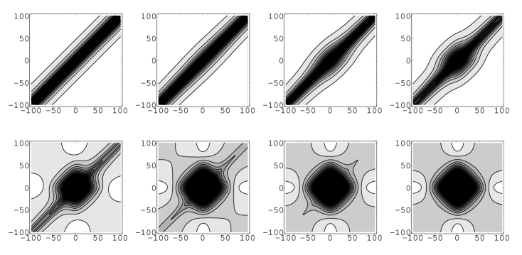
Figure 2: Plots of the $N$x$N$ matrix $U$ at different RG scales $\ell$. Here the number of frequency divisions $N\!=\!200$, and the value of the other parameters are $\lambda\!=\!4$, $\Lambda_{0}\!=\!100$, $\omega_{E}\!=\!10$, and $u_{0}\!=\!0.1$. Panels correspond to $\ell$ = 0, 1, 2, 2.5, 3, 3.13, 3.157, 3.172. The scale $2W_{c}\approx 40$ distinguishes the high and low frequencies close to $\ell_{c}$.

In the strong-coupling regime ($\lambda>1$) the situation is rather different. Fig. 2 shows the numerical results for the full solution of the RG flow for parameters in strong coupling. The form of the matrix ${\bf U}(\ell)$ is very different from the weak-coupling limit and the important scale separating the high and low energy physics is $2W_{c}$. We have seen that for $\lambda<1$ the characteristic energy scale that separates high from low energy physics is $\omega_{E}$. When $\lambda>1$ we expect $W_{c}>\omega_{E}$ in which case $\omega_{E}$ is not the characteristic energy scale of the instability. Instead we expect $W_{c}$ to act as the characteristic energy scale in separating the low and high energy physics. Thus, it is natural to make the following ansatz:

$$\phi(\omega)=\left\{\begin{array}[]{ll}\phi_{0}&\hskip 14.22636pt{\rm if}\ \ \ |\omega|<2W_{c}\\ 0&\hskip 14.22636pt{\rm if}\ \ \ |\omega|>2W_{c}\\ \end{array}\right.\,.$$ (48)

where $\phi_{0}$ is an unknown. Since, as discussed previously, $\mu^{*}$ is bounded from above, the electron-electron interaction will play a minimal role in the problem and can be disregarded.

In this regime (27) becomes ($\phi_{0}\neq 0$):

$$Z_{c}(0)=2\lambda\omega^{2}_{E}\int_{0}^{2W_{c}}\frac{d\omega}{\pi}\int_{W_{c}}^{+\infty}d\Lambda\frac{1}{(\omega^{2}+\Lambda^{2})\,(\omega^{2}+\omega_{E}^{2})}\approx\frac{2\lambda}{\pi}\left(\frac{\pi\omega_{E}}{2W_{c}}-\frac{\pi\omega_{E}^{2}}{4W_{c}^{2}}\right)\,.$$ (49)

But from (14) we have $Z_{c}(0)\approx 1+\lambda(\omega_{E}/W_{c})-\lambda(\omega_{E}/W_{c})^{2}$, which substituted in (49) gives

$$W_{c}\approx\sqrt{\lambda}\omega_{E}\,,$$ (50)

the strong coupling result of Eliashberg equation found by Allen and Dynes allen .

III Discussion and conclusion

We have numerically solved the RG equations for the flow of the BCS coupling matrix for interacting electrons coupled to phonons, for the case of circular Fermi surface and Einstein phonons. Fig. 3 shows the result for the energy scale of divergence in the Cooper channel, for a range of $\lambda$, and the expected analytical result at weak and strong coupling limits. One can clearly see that the approximate analytical solutions, based on the evolution of the coupling matrix under the RG, give a very good description of the superconducting gap in the asymptotic limits. Thus, our RG scheme can used as an alternative way to solve for the superconducting properties of a Fermi liquid and is in full agreement with Eliashberg’s theory.

Figure 3: Plot of $W_{c}$ ($\sim$ superconducting gap) in units of $\omega_{E}$ versus $\lambda$ (black circles) ($N=200$, $\Lambda_{0}=100$, $\omega_{E}=10$, $u_{0}=0.1$). The dashed line is the fit at small $\lambda$’s using the MacMillan formula and the solid line is the fit to $\sqrt{\lambda}$ at large $\lambda$’s (Allen-Dynes).

Unlike mean-field approaches like Eliashberg theory, the RG approach, when solved numerically, can be easily extended to any shape of the Fermi surface or anisotropic phonons. It also addresses the question of competition between different types of instabilities, as was done extensively for the case without phononszanchi ; halboth ; marston . Furthermore, the approach presented here at zero temperature can be easily extended to finite temperature.

References

• (1) S.-W. Tsai, A. H. Castro Neto, R. Shankar, and D. K. Campbell, “Renormalization Group Approach to Strong-Coupled Superconductors”, to appear in Phys.Rev.B.
• (2) R. Shankar, Rev. Mod. Phys. 68, 129 (1994).
• (3) A. Lanzara, et al., Nature 412, 510 (2001); X. J. Zhou, et al., “Multiple Bosonic Mode Coupling in Electron Self-Energy of (La2-xSrx)CuO4, cond-mat/0405130.
• (4) R. H. McKenzie, Science 278, 820 (1997).
• (5) H. J. Choi, M. L. Cohen, and S. G. Louie, Physica C385, 66 (2003).
• (6) A. Deppeler, and A. J. Millis, Phys. Rev. B 65, 224301 (2002).
• (7) J. E. Han, O. Gunnarsson, and V. H. Crespi, Phys. Rev. Lett. 90, 167006 (2003).
• (8) G. M. Eliashberg, Zh. Eksp. Teor. Fiz. 38, 966 (1960) [Sov. Phys. JETP 11, 696 (1960)].
• (9) A. B. Migdal, Zh. Eksp. Teor. Fiz. 34, 1438 (1958) [Sov. Phys. JETP 7, 996 (1958)].
• (10) See, J. P. Carbotte, Rev. Mod. Phys. 62, 1027 (1990), and references therein.
• (11) W. L. McMillan, Phys. Rev. 167, 331 (1968).
• (12) P. B. Allen, and R. C. Dynes, Phys. Rev. B 12, 905 (1975).
• (13) P. Morel and P. W. Anderson, Phys. Rev. 125, 1263 (1962).
• (14) D. Zanchi, and H. J. Schulz, Phys. Rev. B 61, 13609 (2000);
• (15) C. J. Halboth and W. Metzner, Phys. Rev. B 61, 7364 (2000);
• (16) S.-W. Tsai and J. B. Marston, Can. J. Phys. 79 1463 (2001).