Kinetics of the Wako–Saitô–Muñoz–Eaton Model of Protein Folding

Abstract

We consider a simplified model of protein folding, with binary degrees of freedom, whose equilibrium thermodynamics is exactly solvable. Based on this exact solution, the kinetics is studied in the framework of a local equilibrium approach, for which we prove that (i) the free energy decreases with time, (ii) the exact equilibrium is recovered in the infinite time limit, and (iii) the folding rate is an upper bound of the exact one. The kinetics is compared to the exact one for a small peptide and to Monte Carlo simulations for a longer protein, then rates are studied for a real protein and a model structure.

Many experimental findings on the folding of small proteins suggest a strong relationship between the structure of the native state (the functional state of the protein) and the folding kinetics (see e.g. Baker ; OnuchicWolynes and refs. therein), and several theoretical models have been proposed which aim to elucidate the protein folding kinetics on the basis of this relationship. Among these, three studies appeared in 1999 in the same PNAS issue Finkelstein ; AlmBaker ; ME3 , all of them based on models with binary (ordered/disordered) degrees of freedom associated to each aminoacid or peptide bond (the bond between consecutive aminoacids). The third of these works ME3 is particularly interesting because it is based on a model with remarkable mathematical properties which make it possible to obtain exact results. It is a one–dimensional model, with long–range, many–body interactions, where a binary variable is associated to each peptide bond. Two aminoacids can interact only if they are in contact in the native state and all the peptide bonds between them are in the ordered state. Moreover an entropic cost is associated to each ordered bond.

A homogeneous version of the model was first introduced in 1978 by Wako and Saitô WS1 ; WS2 , who solved exactly the equilibrium thermodynamics. The full heterogeneous case was later considered by Muñoz, Eaton and coworkers ME1 ; ME2 ; ME3 , who introduced the single (double, triple) sequence approximations, i.e. they considered only configurations with at most one (two, three) stretches of consecutive ordered bonds, for both the equilibrium and the kinetics. They applied the model to the folding of a 16–aminoacid $\beta$–hairpin ME1 ; ME2 , and to a set of 22 proteins ME3 . The equilibrium problem has been subsequently studied in Amos , with exact solutions for homogeneous $\beta$–hairpin and $\alpha$–helix structures, mean field approximation and Monte Carlo simulations. The exact solution for the equilibrium in the full heterogeneous case was given in BP . Moreover, in P it was shown that the equilibrium probability has an important factorization property, which implies the exactness of the cluster variation method (CVM) Kikuchi ; An ; TopicalReview , a variational method for the study of lattice systems in statistical mechanics. Recently, the model has been used to study the kinetics of the photoactive yellow protein ItohSasai1 ; ItohSasai2 and the free energy profiles and the folding rates of a set of 25 two–state proteins HenryEaton . It is also interesting that the WSME model, and the technique developed in BP , have found an application in a problem of strained epitaxy TD1 ; TD2 ; TD3 .

The ultimate purpose of this class of models being the study of the kinetics, under the assumption that it is mainly determined by the structure of the native state, it is worth asking whether the exact solution developed for the equilibrium can be extended to the kinetics. Strictly speaking, in the general case an exact solution for the kinetics can not be achieved. Nevertheless, thanks to the factorization property proved in P , it is possible to devise a local equilibrium approach for the kinetics which can be proved to yield the exact equilibrium state in the infinite time limit. It is the aim of the present Letter to illustrate this approach and its properties, and to discuss its accuracy and its possible applications.

The WSME model describes a protein of $N+1$ aminoacids as a chain of $N$ peptide bonds (connecting consecutive aminoacids) that can live in two states (native and unfolded) and can interact only if they are in contact in the native structure and if all bonds in the chain between them are native. To each bond is associated a binary variable $m_{i}$, $i\in\{1,\ldots,N\}$, with values $0,1$ for unfolded and native state respectively. The effective free energy of the model (sometimes improperly referred to as Hamiltonian) reads

$$H_{N}(m)=\sum_{i=1}^{N-1}\sum_{j=i+1}^{N}\epsilon_{i,j}\Delta_{i,j}\prod_{k=i}^{j}m_{k}-RT\sum_{i=1}^{N}q_{i}(1-m_{i})$$ (1)

where $R$ is the gas constant and $T$ the absolute temperature. The first term assigns an energy $\epsilon_{i,j}<0$ to the contact (defined as in ME3 ; BP ) between bonds $i$ and $j$ if this takes place in the native structure ($\Delta_{i,j}=1$ in this case and $\Delta_{i,j}=0$ otherwise). The second term represents the entropic cost $q_{i}>0$ of ordering bond $i$.

A crucial step in the exact solution of the equilibrium problem BP ; P is a mapping onto a two–dimensional model through the introduction of the variables $x_{i,j}\doteq\prod_{k=i}^{j}m_{k}$ which satisfy the short–range constraints $x_{i,j}=x_{i,j-1}x_{i+1,j}$ for $1\leq i<j\leq N$. These can be associated to the nodes of a triangular shaped portion $\Lambda$ of a two–dimensional square lattice, defined by $\Lambda=\{(i,j)\in\mathbb{N}^{2}:1\leq i\leq j\leq N\}$. Let ${\cal{C}}_{\Lambda}$ be the set of all configurations $x$ on $\Lambda$ that fulfil previous constraints and rewrite the effective free energy (divided by $RT$ and leaving apart an additive constant) in the form

$$H_{\Lambda}(x)=\sum_{(i,j)\in\Lambda}h_{i,j}x_{i,j}.$$ (2)

The corresponding Boltzmann distribution, which will be denoted by $p_{\Lambda}^{e}$, has been shown P to factor as

$$p^{e}_{\Lambda}(x)=\prod_{\alpha\in\cal{A}}[p^{e}_{\alpha}(x_{\alpha})]^{a_{\alpha}}.$$ (3)

Here $\cal{A}$ is a set of local clusters $\alpha\subset\Lambda$ made of all square plaquettes ($a_{\alpha}=1$), the triangles lying on the diagonal boundary ($a_{\alpha}=1$) and their intersections, that is internal nearest–neighbour pairs ($a_{\alpha}=-1$) and single nodes ($a_{\alpha}=1$). For each cluster $\alpha\in\cal{A}$ we denote by $x_{\alpha}$ ($x_{\Lambda\setminus\alpha}$) the projection of $x$ onto $\alpha$ ($\Lambda\setminus\alpha$), by $\cal{C}_{\alpha}$ the set of all configurations on $\alpha$ that are projections of configurations on $\Lambda$, and define the cluster probability as the marginal distribution

$$p_{\alpha}^{e}(x_{\alpha})\doteq\sum_{x_{\Lambda\setminus\alpha}}p_{\Lambda}^{e}(x).$$ (4)

As a consequence of Eq. (3), the equilibrium problem can be solved exactly P by means of the CVM. Let ${\cal{D}}_{\Lambda}$ be the set of all cluster probabilities $p$ relative to $\cal{A}$ satisfying the compatibility conditions $p_{\beta}(x_{\beta})=\sum_{x_{\alpha\setminus\beta}}p_{\alpha}(x_{\alpha})$ for $\alpha,\beta\in\cal{A}$ and $\beta\subset\alpha$. Since the Boltzmann distribution minimizes the free energy and factors, restricting the variational principle to distributions with the same property one finds that $p^{e}\in{\cal{D}}_{\Lambda}$ is the minimum of the variational free energy

$$F_{\Lambda}[p]=\sum_{\alpha\in\cal{A}}\sum_{x_{\alpha}}a_{\alpha}[\ln p_{\alpha}(x_{\alpha})+h_{\alpha}(x_{\alpha})]p_{\alpha}(x_{\alpha})$$ (5)

with respect to $p\in{\cal{D}}_{\Lambda}$. Here $h_{\alpha}$ are defined by $h_{\alpha}(x_{\alpha})\doteq\sum_{(i,j)\in\alpha}h_{i,j}x_{i,j}$ and it follows that $H_{\Lambda}(x)=\sum_{\alpha\in\cal{A}}a_{\alpha}h_{\alpha}(x_{\alpha})$. This variational approach is not the most efficient way to solve the equilibrium problem, which is handled in BP by the transfer matrix method. Nevertheless it is a good starting point for a very accurate treatment of the kinetics.

Our kinetic problem will be formulated in the framework of a master equation approach. Denoting by $W_{\Lambda}(x^{\prime}\to x)$ the transition probability per unit time from the state $x^{\prime}$ to $x\not=x^{\prime}$, we have to solve

$$\frac{d}{dt}p^{t}_{\Lambda}(x)=\sum_{x^{\prime}\in{\cal{C}}_{\Lambda}}W_{\Lambda}(x^{\prime}\to x)p^{t}_{\Lambda}(x^{\prime})$$ (6)

where $W_{\Lambda}(x\to x)$ is such that $\sum_{x\in{\cal{C}}_{\Lambda}}W_{\Lambda}(x^{\prime}\to x)=0$. If the principle of detailed balance holds, i.e. $W_{\Lambda}(x^{\prime}\to x)p^{e}_{\Lambda}(x^{\prime})=W_{\Lambda}(x\to x^{\prime})p^{e}_{\Lambda}(x)$, and $W_{\Lambda}$ is irreducible, then the expected equilibrium is reached.

The above problem is in general not exactly solvable and in order to overcome this difficulty, we shall assume local equilibrium Kawasaki ; AdvPhys , that is we shall assume that, provided the initial condition $p^{0}_{\Lambda}$ factors according to Eq. (3) as the equilibrium probability, the solution $p^{t}_{\Lambda}$ of the master equation factors in the same way at any subsequent time. With this simplification the master equation yields Thesis ; Prep , for the cluster probabilities,

$$\frac{d}{dt}p^{t}_{\alpha}(x_{\alpha})=\sum_{x^{\prime}\in{\cal{C}}_{\Lambda}}W_{\alpha}(x^{\prime}\to x_{\alpha})\prod_{\beta\in\cal{A}}[p^{t}_{\beta}(x_{\beta}^{\prime})]^{a_{\beta}},$$ (7)

where

$$W_{\alpha}(x^{\prime}\to x_{\alpha})\doteq\sum_{x_{\Lambda\setminus\alpha}}W_{\Lambda}(x^{\prime}\to x).$$ (8)

One can show Thesis ; Prep that the above evolution preserves the compatibility conditions between the cluster probabilities and that the free energy is not increasing in time,

$$\frac{d}{dt}F_{\Lambda}[p^{t}]\leq 0$$ (9)

(equality holding if and only if $p^{t}=p^{e}$). Since $p^{e}$ minimizes the free energy, it follows by Lyapunov’s theorem that the exact equilibrium probability is recovered in the infinite time limit,

$$\lim_{t\to+\infty}p^{t}=p^{e}.$$ (10)

It is important to stress that in previous approximations ME2 for the kinetics the above condition was not satisfied, and the behaviour of the free energy was not discussed.

Moreover, denoting by $-k$ ($k>0$) the largest eigenvalue of the jacobian matrix of the r.h.s. in (7) evaluated at equilibrium, we have that Prep for all $p^{0}\in{\cal{D}}_{\Lambda}$ there exist functions $R_{\alpha}^{t}$ defined on ${\cal{C}}_{\alpha}$, $\forall~{}\alpha\in\cal{A}$, having a finite limit for $t\to+\infty$ and such that

$$p^{t}_{\alpha}=p^{e}_{\alpha}+\mbox{e}^{-kt}R^{t}_{\alpha},$$ (11)

which allows to define the equilibration rate as $k$. It can also be shown Prep that this approximate equilibration rate is an upper bound of the exact one, which can be intuitively understood by observing that the local equilibrium assumption implies that we are dealing with an evolution in a restricted probability space.

It is also important to observe that, since the cluster probabilities can be written P as linear functions of the expectation values

$$\xi_{i,j}(t)\doteq\langle x_{i,j}\rangle(t)=\sum_{x\in{\cal{C}}_{\Lambda}}x_{i,j}\prod_{\alpha\in\cal{A}}[p^{t}_{\alpha}(x_{\alpha})]^{a_{\alpha}}$$ (12)

(the probability of the stretch from $i$ to $j$ being native) Eq. (7) can be rewritten as

$$\frac{d}{dt}\xi(t)=f(\xi(t))$$ (13)

with a suitable function $f$, and the kinetic problem is complete with an initial condition $\xi(0)$.

A couple of important remarks are in order here. First of all, for the single “bond–flip” kinetics which will be used in the following, Eq. (13) turns out to be of polynomial complexity and our approach yields a reduction of computational complexity which makes the kinetic problem tractable. This might not be true for other, more complicated, choices of the transition probability, due to the summation in Eq. (8). In addition, we observe that the whole approach can be reformulated in a discrete time framework Prep ; Thesis .

In order to assess the accuracy of our approach, we have applied it to the kinetics of the 16 residues C-terminal $\beta$–hairpin of streptococcal protein G B1 ME1 ; ME2 ; BP . For such a simple system it is easy to compute the exact time evolution of $\xi$, denoted by $\xi^{ex}$, which we compare to our results. Parameters for the effective free energy are taken from BP , $T$ is set to 290 K, the initial condition is the equilibrium state at infinite temperature and the transition probability is specified by

$$W_{\Lambda}(x\to x^{\prime})=\frac{\tau^{-1}}{1+\exp[H_{\Lambda}(x^{\prime})-H_{\Lambda}(x)]}$$ (14)

if $x$ and $x^{\prime}$ differ by exactly one bond, that is by the value of a single $m_{i}$ variable. Here $\tau$ is a microscopic time scale , $W_{\Lambda}(x\to x)=-\sum_{x^{\prime}\neq x}W_{\Lambda}(x\to x^{\prime})$, and $W_{\Lambda}(x\to x^{\prime})=0$ if $x$ and $x^{\prime}$ differ by more than one bond.

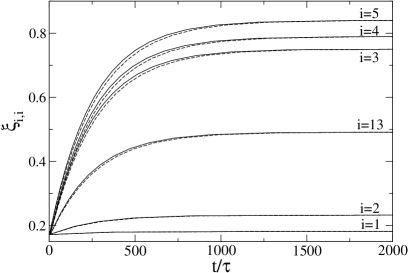
Figure 1: Probability of $\beta$-hairpin bond $i$ being native, versus time. Solid lines: our results, dashed line: exact results.

In Fig. 1 we report our results for the behaviour of the probability $\xi_{i,i}$ of bond $i$ being native, as a function of time. We do not report curves for every value of $i$, since the curves for $i=5$ to 12 (corresponding to most of the hydrophobic core) are almost indistinguishable on the graph scale, and in addition $\xi_{15,15}$ and $\xi_{14,14}$ are almost indistinguishable from $\xi_{1,1}$ and $\xi_{2,2}$ respectively (which follows from the symmetry of the hairpin). A more quantitative measure of the accuracy of our approximation is

$$\max_{t\in\mathbb{R}_{+}}\max_{(i,j)\in\Lambda}|\xi_{i,j}(t)-\xi_{i,j}^{\rm ex}(t)|$$ (15)

which takes the value $1.6\cdot 10^{-2}$, which is attained for $(i,j)=(5,12)$ and $t\simeq 260~{}\tau$. Equilibration rates are also easily computed in our approach. In the case of Fig. 1 we obtain $k\simeq 3.93\cdot 10^{-3}~{}\tau^{-1}$, while the exact value is $3.72\cdot 10^{-3}~{}\tau^{-1}$.

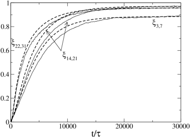
Figure 2: Probability of $\alpha$–helix structures in headpiece subdomain being native, versus time. Dashed lines: our results, solid lines: Monte Carlo simulations.

In order to test our approach on a longer protein, we have considered the headpiece subdomain of the F-actin-binding protein villin (pdb code 1VII) and compared our solution with Monte Carlo simulations (in this case the exact solution is not feasible). The headpiece subdomain contains three $\alpha$–helices going from bond $3$ to $7$, form bond $14$ to $17$ and from bond $22$ to $31$. Fig. 2 shows the probabilities $\xi_{3,7}$, $\xi_{14,17}$ and $\xi_{22,31}$ versus time at the temperature of $300$ K. Parameters for the effective free energy are taken as in ME3 ; BP , the energy scale is chosen in order to have $\frac{1}{N}\sum_{i=1}^{N}\xi_{i,i}=1/2$ at equilibrium at the experimental transition temperature $T=343$ K 1VII.bib . The agreement is still remarkably good and similar results are obtained for proteins BBL and CI2 (pdb codes 1BBL and 1COA respectively).

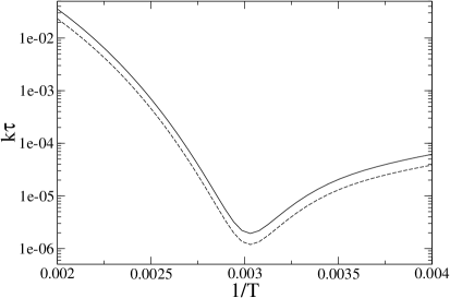
Figure 3: PIN1 equilibration rate versus inverse temperature. Solid lines: Glauber kinetics, dashed line: Metropolis kinetics.

Fig. 3 reports the equilibration rates as a function of temperature for the WW domain of protein PIN1 (pdb code 1I6C) computed using two different choices for the transition probability: Glauber kinetics, corresponding to Eq. (14) and Metropolis kinetics, where Eq. (14) is replaced by

$$W_{\Lambda}(x\to x^{\prime})=\tau^{-1}\exp[H_{\Lambda}(x)-H_{\Lambda}(x^{\prime})]$$ (16)

if $H_{\Lambda}(x^{\prime})\geq H_{\Lambda}(x)$ and $W_{\Lambda}(x\to x^{\prime})=\tau^{-1}$ otherwise. Here $q_{i}$ are chosen as in Cecco , $\epsilon_{i,j}$ as in ME3 ; BP and the energy scale in order to have the transition at the experimental temperature of $332$ K Gruebele . It can be seen that the detailed choice of the kinetics affects only marginally the behaviour of the equilibration rates, which is in very good qualitative agreement with the experimental results Gruebele . The same behaviour is obtained for protein CI2.

Finally, given the observed correlation between experimental equilibration rates and structural characteristics like the absolute contact order ACO $=\frac{1}{N_{c}}\sum_{i<j}\Delta_{i,j}(j-i+1)$ ACO ($N_{c}$ is the total number of contacts, $j-i+1$ the distance in sequence between aminoacids involved in contact $(i,j)$), we have computed the rates predicted by our approach for a simple model structure, an antiparallel $\beta$–sheet made of 4 strands, varying the length $r$ of the strands. In this case the ACO is equal to $r$, while the relative contact order is a constant. We have used Glauber kinetics, $q_{i}=2$ and $\epsilon_{i,j}/(RT)$ independent of $(i,j)$ and such that $\frac{1}{N}\sum_{i=1}^{N}\xi_{i,i}=1/2$ at equilibrium. Results are reported in Fig. 4, which shows an almost perfect linear correlation between $\log k$ and the ACO.

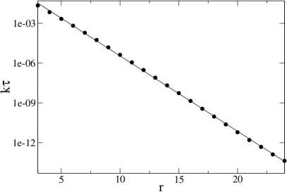
Figure 4: Equilibration rate for a $\beta$–sheet of four strands versus absolute contact order. Dots: our results, line: exponential fit.

In conclusion, we can say that the local equilibrium approach for the kinetics of the WSME model gives very accurate results with respect to the exact ones. It allows to compute equilibration rates, and hence to explore the relationship between kinetics and structure of the native state. The detailed evolution is also available, which can be very useful to study folding pathways. Work is in progress on several two–state folders and on the effect of mutations. Details of a few mathematical proofs will be given in Prep .

- (1) D. Baker, Nature (London) 405, 39 (2000).
- (2) J.N. Onuchic and P.G. Wolynes, Curr. Opin. Struct. Biol. 14, 70 (2004).
- (3) O.V. Galzitskaya and A.V. Finkelstein, Proc. Natl. Acad. Sci. U.S.A. 96, 11299 (1999).
- (4) E. Alm and D. Baker, Proc. Natl. Acad. Sci. U.S.A. 96, 11305 (1999).
- (5) V. Muñoz and W.A. Eaton, Proc. Natl. Acad. Sci. U.S.A. 96, 11311 (1999).
- (6) H. Wako and N. Saitô, J. Phys. Soc. Jpn 44, 1931 (1978).
- (7) H. Wako and N. Saitô, J. Phys. Soc. Jpn 44, 1939 (1978).
- (8) V. Muñoz, P.A. Thompson, J. Hofrichter and W.A. Eaton, Nature 390, 196 (1997).
- (9) V. Muñoz et al., Proc. Natl. Acad. Sci. U.S.A. 95, 5872 (1998).
- (10) A. Flammini, J.R. Banavar and A. Maritan, Europhys. Lett. 58, 623 (2002).
- (11) P. Bruscolini and A. Pelizzola, Phys. Rev. Lett. 88, 258101 (2002).
- (12) A. Pelizzola, J. Stat. Mech., P11010 (2005).
- (13) R. Kikuchi, Phys. Rev. 81, 988 (1951).
- (14) G. An, J. Stat. Phys. 52, 727 (1988).
- (15) A. Pelizzola, J. Phys. A 38, R309 (2005).
- (16) K. Itoh and M. Sasai, Proc. Natl. Acad. Sci. U.S.A. 101, 14736 (2004).
- (17) K. Itoh and M. Sasai, Chem. Phys. 307, 121 (2004).
- (18) E.R. Henry, W.A. Eaton, Chem. Phys. 307, 163 (2004).
- (19) V.I. Tokar and H. Dreyssé, Phys. Rev. E 68, 011601 (2003).
- (20) V.I. Tokar and H. Dreyssé, J. Phys. Cond. Matter 16, S2203 (2004).
- (21) V.I. Tokar and H. Dreyssé, Phys. Rev. E 71, 031604 (2005).
- (22) M. Zamparo and A. Pelizzola, in preparation.
- (23) K. Kawasaki, in Phase Transitions and Critical Phenomena, vol. 2, ed. C. Domb and M.S. Green (Academic, London, 1972).
- (24) J.-F. Gouyet, M. Plapp, W. Dieterich and P. Maass, Adv. Phys. 52, 523 (2003).
- (25) M. Zamparo, thesis, Politecnico di Torino (2005).
- (26) R. Kikuchi, Progr. Theor. Phys. Suppl. 35, 1 (1966).
- (27) F. Ducastelle, Progr. Theor. Phys. Suppl. 115, 255 (1994).
- (28) C.J. McKnight et al, J. Mol. Biol. 260, 126 (1996).
- (29) P. Bruscolini and F. Cecconi, Biophys. Chem. 115, 153 (2005).
- (30) M. Jäger et al, J. Mol. Biol. 311, 373 (2001).
- (31) D.N. Ivankov et al, Prot. Sci. 12, 2057 (2003).