Frequency dispersion of photon-assisted shot noise in mesoscopic conductors

Abstract

We calculate the low-frequency current noise for AC biased mesoscopic chaotic cavities and diffusive wires. Contrary to what happens for the admittance, the frequency dispersion is not dominated by the electric response time (the ”RC” time of the circuit), but by the time that electrons need to diffuse through the structure (dwell time or diffusion time). Frequency dispersion of noise stems from fluctuations of the Fermi distribution function that preserve charge neutrality. Our predictions can be verified with present experimental technology.

Charge neutrality in mesoscopic devices is enforced by Coulomb interaction on a time scale ($\tau_{RC}$) given by the product of the resistance and the capacitance scales. The typical time ($\tau_{D}$) for non interacting electron motion is instead fixed by either the dwell or diffusion time, depending on the transparency of the interfaces between the system and the electrodes. The typical physically realized situation is $\tau_{RC}\ll\tau_{D}$: electrons, which would normally slowly diffuse, are pushed to run by the electric fields that they are generating themselves by piling up charge. The consequence is that the typical response time of the device is $\tau^{-1}=\tau_{RC}^{-1}+\tau_{D}^{-1}\approx\tau_{RC}^{-1}$. This has been shown for the frequency dependence of both the admittance Büttiker et al. (1993); Naveh et al. (1999) and the noise Nagaev (1998); Golubev and Zaikin (2004); Nagaev et al. (2004); Hekking and Pekola (2006) in mesoscopic chaotic cavities and diffusive wires. The inverse of the diffusion time appears instead as the relevant energy scale for the voltage or temperature dependence for both the conductance and the noise in superconducting/normal metals hybrid systems Volkov et al. (1993); Hekking and Nazarov (1994); Belzig and Nazarov (2001); Houzet and Pistolesi (2004). Indeed, in this case the energy dependence is due to interference of electronic waves that does not induce charge accumulation in the systems. To our knowledge, in normal metallic structures a dispersion on the inverse diffusion time scale has been predicted so far only for the third moment of current fluctuations Nagaev et al. (2004) and for the finite frequency thermal noise response to an oscillating heating power Reulet and Prober (2005). An alternative, and less investigated possibility, is to study the low frequency current noise as a function of the frequency $\Omega$ of an external AC bias. The noise for a quantum point contact was calculated a decade ago Lesovik and Levitov (1994) and later measured Schoelkopf et al. (1997); Reydellet et al. (2003). Since the quantum point contact is very short, electron diffusion does not introduce any additional time scale in the problem and the resulting frequency dispersion is simply linear Lesovik and Levitov (1994). More recently, the noise for an AC biased chaotic cavity was considered Rychkov et al. (2005); Polianski et al. (2005) in the limit of small fields $eV/\hbar\Omega\ll 1$ ($V$ is the amplitude of the AC bias and $e$ is the electron change). The authors of Ref. Rychkov et al. (2005) found that the noise disperse only on the $\tau$ scale, that is the combination of the diffusion and the electric response time. This should be contrasted with the result of Ref. Altshuler et al. (1994) where the noise in a diffusive wire was studied when the conductor was biased by a short voltage pulse. Even if the dispersion of the noise is not considered in that paper, the authors find that the ratio of the diffusion time to the time duration of the pulse may affect the observed noise. This indicate that a dispersion of the noise on the external frequency could be present.

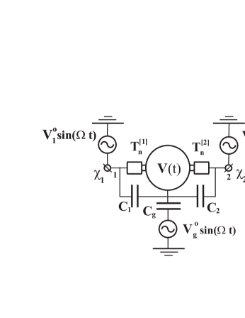
Figure 1: Schematic of the system. A chaotic cavity connected to the electrodes through arbitrary coherent connectors characterized by a set of transparencies $\{T_{n}\}$.

In this paper we derive analytical expressions for the photon-assisted noise in chaotic cavities [Eq. (13) in the following] and numerical results for diffusive wires. We show that the noise depends on the AC frequency $\Omega$ on the diffusion time scale. We take into account the Coulomb response that guarantees charge neutrality over times longer than $\tau_{RC}$. Within our calculation, the admittance has no structure at $\Omega\approx 1/\tau_{D}$, while the derivative of the noise with respect to the frequency shows a clear maximum.

We start by considering a chaotic cavity (see Fig. 1) connected to two metallic leads through two barriers characterized by a set of transparencies $\{T_{n}^{k}\}$ where $k$ takes the value 1 or 2. We define the conductances $G_{k}=G_{Q}\sum_{n}T_{n}^{k}$, the total conductance $G=G_{1}G_{2}/(G_{1}+G_{2})$, and a dwell time $\tau_{D}=2\pi\hbar G_{Q}/(G_{1}+G_{2})\delta$, where $\delta$ is the level spacing of the cavity and $G_{Q}=e^{2}/(2\pi\hbar)$. We assume that the dwell time is much shorter that the inelastic time. We also assume that $G_{\Sigma}=G_{1}+G_{2}\gg G_{Q}$ so that we can use semiclassical theory to describe transport and neglect Coulomb blockade effects. The cavity is coupled capacitively to the leads through the capacitances $C_{k}$ and to a gate through $C_{g}$. One can then define the typical electric response time as $\tau_{RC}=C_{\Sigma}/G$ where $C_{\Sigma}=C_{1}+C_{2}+C_{g}$. If linear dimension of the cavity $L$ are much larger than the Fermi wavelength $\lambda_{F}$, the ratio $\tau_{RC}/\tau_{D}\approx\delta/E_{C}\approx(\lambda_{F}/L)^{d-1}\ll 1$ where $E_{C}=e^{2}/C_{\Sigma}$ is the Coulomb energy and $d=2$ or $3$ is the dimension of the cavity. Three different time dependent voltage biases are applied to the gate and the two contacts ($V_{g}$, $V_{1}$, and $V_{2}$), clearly the current depends only on two voltage differences, we keep the three voltages to simplify the notation. The cavity resistance is negligible with respect to the contact resistances so that we can assume a uniform electric potential inside.

We begin by considering a very simple model of charge transport, where diffusion and electric drift are described classically. The charge $Q$ in the cavity is related to the electric potential $V$ of the cavity itself by the relation $Q=\sum_{k}C_{k}(V-V_{k})$, where $k=1$, $2$, and $g$. The equation of motion for $Q$ is then

$$\partial_{t}Q+Q/\tau_{D}+I_{1}+I_{2}=0,$$ (1)

where $I_{k}=G_{k}(V-V_{k})$. The equation can be conveniently solved in terms of $V(\omega)$, the Fourier transform of the cavity potential:

$$V(\omega)={\tau/\tau_{D}\over 1-i\omega\tau}\sum_{k=1,2,g}V_{k}(\omega)\left[\alpha_{k}{\tau_{D}\over\tau_{RC}}+(1-i\omega\tau_{D}){C_{k}\over C_{\Sigma}}\right],$$

where we defined $\alpha_{k}=G_{k}/G_{\Sigma}$ for $k=1$ or $2$, and $\alpha_{g}=0$. When $\tau_{RC}\ll\tau_{D}$, the response time $\tau=\tau_{RC}\tau_{D}/(\tau_{RC}+\tau_{D})$ is simply given by $\tau_{RC}$. The admittance has a similar frequency dependence. For $\tau_{RC}\ll\tau_{D}$ and $\omega\tau\ll 1$ one thus finds the very simple result

$$V(\omega)=\sum_{k}\alpha_{k}V_{k}(\omega),$$ (2)

and $I_{1}(\omega)=-I_{2}(\omega)=G_{\Sigma}\alpha_{1}\alpha_{2}(V-V_{1})$: charge neutrality is perfectly enforced for low frequency drive. As it follows from Eq. (1), only $I_{k}$ is finite, since $Q$ and $\partial_{t}Q$ vanish in this limit. In the following we will consider this experimentally relevant low driving-frequency limit $\Omega\tau_{RC}\ll 1$, which will enable us to use the $\omega\ll 1/\tau_{RC}$ response for $V(\omega)$.

Let us now consider the noise. We use the semiclassical description of non-equilibrium transport provided by the time dependent Usadel equations Usadel (1970); Larkin and Ovchinninkov (1986):

$$D\nabla(\check{\cal G}\nabla\check{\cal G})+\left[i\hbar(\partial_{t_{1}}+\partial_{t_{2}})+eV(t_{1})-eV(t_{2})\right]\check{\cal G}=0,$$ (3)

where $D$ is the diffusion coefficient in the cavity and the Keldysh Green’s function satisfies the normalization condition:

$$\sum_{l}\int_{-\infty}^{+\infty}\!\!\!\!\!\!dt\ \check{\cal G}_{il}(t_{1},t)\check{\cal G}_{lj}(t,t_{2})=\delta_{ij}\delta(t_{1}-t_{2})\,.$$ (4)

Since the conductance is controlled by the contacts, $\check{\cal G}(t_{1},t_{2})$ is uniform in the cavity. Eq. (3) can then be integrated on the volume of the cavity, and relate $\check{\cal G}$ to the current through the interfaces Nazarov (1999a). The equation for $\check{\cal G}$ takes then the form of a charge conservation equation:

$$\sum_{k}{\check{\cal I}_{k}}-{i\tau_{D}}\left[i\hbar(\partial_{t_{1}}+\partial_{t_{2}})+eV(t_{1})-eV(t_{2})\right]{\check{\cal G}}=0,$$ (5)

where the voltage in the cavity is given by the electroneutrality condition (2) and

$${\check{\cal I}_{k}}={G_{Q}\over G_{\Sigma}}\sum_{n}{T_{n}^{[k]}[\check{\cal G}_{k},\check{\cal G}]\over 4+T_{n}^{[k]}(\{\check{\cal G}_{k},\check{\cal G}\}-2)}$$ (6)

are the spectral currents that relate the Green’s function of the electrodes $\check{\cal G}_{k}$ to the Green function of the cavity Nazarov (1999b). The form of $\check{\cal G}_{k}$ is given by the equilibrium solution for metallic leads of Eq. (5), explicitly, in presence of a time dependent potential, one has:

$$\check{\cal G}_{ok}(t_{1},t_{2})=\left(\begin{array}[]{cc}\delta(t_{1}-t_{2})&2F_{k}(t_{1},t_{2})\\ 0&-\delta(t_{1}-t_{2})\end{array}\right)$$ (7)

where $\hbar\partial_{t}\phi_{k}(t)=eV_{k}(t)$, $F_{k}(t_{1},t_{2})=e^{i\phi_{k}(t_{1})}F_{eq}(t_{1}-t_{2})e^{-i\phi_{k}(t_{2})}$, and $F_{eq}(t)=\int(d\varepsilon/2\pi)e^{i\varepsilon t/\hbar}\tanh(\varepsilon/2T)]=-i{\cal P}T/\sinh(\pi Tt/\hbar)$, with $T$ being the temperature ($k_{B}=1)$.

In order to calculate the noise we need to modify the Green’s function of the electrodes by introducing two counting fields Levitov et al. (1996); Nazarov (1999a):

$$\check{\cal G}_{k}=e^{i\sigma_{x}\chi_{k}/2}\check{\cal G}_{ok}e^{-i\sigma_{x}\chi_{k}/2}$$ (8)

where $\sigma_{x}$ is a Pauli matrix. Solving Eq. (5) together with Eq. (2) gives the value of $\check{\cal G}$ from which, using Eq. (6) one can derive the counting field dependent current: $I_{k}(t,\chi_{1},\chi_{2})=G_{k}{\rm Tr}\{\sigma_{x}\check{\cal I}_{k}(t,t)\}/2$. Derivatives with respect to $\chi_{1}-\chi_{2}$ give all the moments of current fluctuations. We assume that the potential difference between the two leads is harmonically oscillating at frequency $\Omega$. Then the time average over the period $2\pi/\Omega$ of $I_{k}(t)$ and $-i\partial I_{k}(t)/\partial(\chi_{1}-\chi_{2})$ gives the DC current and the low frequency noise, respectively.

Let us first discuss briefly the current. For vanishing $\chi_{k}$, $\check{\cal G}$ has the form given by Eq. (7) and it depends on a single function: $F(t_{1},t_{2})$. It is convenient to change gauge by defining $F(t_{1},t_{2})=e^{i\phi(t_{1})}\,\tilde{F}(t_{1},t_{2})\,e^{-i\phi(t_{2})}$ where $\hbar\partial_{t}\phi(t)=eV(t)$, and introducing new time variables $t_{-}=t_{2}-t_{1}$ and $t_{+}=(t_{1}+t_{2})/2$. $\tilde{F}(t_{+},t_{-})$ is a periodic function of $t_{+}$: $\tilde{F}(t_{+},t_{-})=\sum_{n}e^{in\Omega t_{+}}F_{n}(t_{-})$ and its explicit expression in terms of the Fourier component of $\tilde{F}^{(k)}$ comes from the solution of the equation of motion (5):

$$F_{n}(t_{-})={\sum_{k}\alpha_{k}F_{n}^{(k)}(t_{-})\over 1+in\Omega\tau_{D}}\,.$$ (9)

Here $F_{n}^{(k)}(t)=F_{eq}(t)J_{n}\left(2A_{k}\sin(\Omega t/2)\right)$, $J_{n}$ are Bessel functions, $A_{k}=e(V^{o}_{k}-V^{o})/(\hbar\Omega)$, and $V^{o}$ are the amplitudes of the AC field: $V_{k}(t)=V_{k}^{o}\sin(\Omega t)$. In order to make a connection with the classical description given by Eq. (1) we relate $\tilde{F}$ to the charge on the cavity:

$$Q(t_{+})=-\left(e/\delta\right)\tilde{F}(t_{-}\rightarrow 0,t_{+})\,.$$ (10)

Usadel equations (5) for $t_{-}\rightarrow 0$ reduces then to the continuity equation (1) for the total charge. Note that when the voltage time dependence (2) is enforced, $Q$ vanishes identically, as it can be verified by calculating the limit $t_{-}\rightarrow 0$ in Eq. (9). On the other hand, the energy distribution function, $\tilde{F}(t_{+},\varepsilon)=\int dt_{-}\tilde{F}(t_{-},t_{+})e^{i\varepsilon t_{-}/\hbar}$, varies periodically in time, and its dependence on the AC driving frequency, $\Omega$, is on the scale of the inverse diffusion time $\tau_{D}^{-1}$. When an electron enters the cavity, after a very short time $\sim\tau_{RC}$, the charge rearranges to keep the cavity neutral, the distribution function, instead, will relax on a much longer time given by $\tau_{D}$. Since zero-frequency noise probes the electronic distribution function, it should depend on the frequency $\Omega$ on the same scale.

To obtain the noise, it is sufficient to expand the Green’s function up to first order in $\chi$: $\check{\cal G}=\check{\cal G}_{o}+\check{\cal G}_{1}i(\chi_{1}-\chi_{2})/2+\dots$, and substitute this expression into Eq. (5) Belzig and Nazarov (2001); Houzet and Pistolesi (2004). The term $\check{\cal G}_{o}$ is given by Eq. (7) with $F$ given by Eq. (9). Note that in principle also $V(\omega)$ could depend on $\chi_{k}$. By going back to the Keldysh action formulation we verified that the corrections are of order higher than one in $\chi_{k}$, they thus do not contribute to the calculation of the noise. In order to fulfil the normalization condition (4) we use the parametrization for $\check{\cal G}_{1}$ proposed in Ref. Kamenev and Andreev (1999):

$$i{\chi}\,\check{\cal G}_{1}=\left(\begin{array}[]{cc}1&F\\ 0&-1\end{array}\right)\left(\begin{array}[]{cc}0&{W}\\ {W^{\prime}}&0\end{array}\right)\left(\begin{array}[]{cc}1&F\\ 0&-1\end{array}\right).$$ (11)

By defining $\chi=\chi_{1}-\chi_{2}$ and choosing $\chi_{1}=\alpha_{2}\chi$, $\chi_{2}=-\alpha_{1}\chi$ we obtain $W^{\prime}=0$ and the kinetic equation for $W$:

$$i(1+\tau_{D}\partial_{t_{+}})W = \sum_{k}\chi_{k}\alpha_{k}\left[(1-\beta_{k})(F\circ F+F_{k}\circ F_{k})\right.$$ (12)

$$+ \left.\beta_{k}(F\circ F_{k}+F_{k}\circ F)\right],$$

where $\beta_{k}=G_{Q}/G_{k}\sum_{n}T_{n}^{(k)}(1-T_{n}^{(k)})$ are the Fano factors of the two junctions and with $\circ$ we indicate time convolution. To obtain the low frequency noise we need $W$ averaged over one period, the $n=0$ Fourier component of Eq. (12) thus suffices for our purpose. Substituting the expression for $W$ into the current definition and evaluating the traces we obtain:

$$S=G_{\Sigma}\sum_{n,l,r}\frac{\hbar\omega_{0}(l+r)\coth\left({\bar{\omega}_{0}(l+r)\over 2T}\right)}{1+\omega_{0}^{2}\tau_{D}^{2}n^{2}}\times$$ (13)

$$\left[{\cal F}\,{\cal J}(A_{1},A_{2})+{\cal F}_{1}\,{\cal J}(A_{1},A_{1})+{\cal F}_{2}\,{\cal J}(A_{2},A_{2})\right]$$

$$+ 2G_{\Sigma}T(1-\beta_{1}\alpha_{2}-\beta_{2}\alpha_{1}),$$

where ${\cal J}(A_{1},A_{2})=J_{n+l}(A_{1})J_{l}(A_{1})J_{r-n}(-A_{2})J_{r}(-A_{2})$, ${\cal F}_{1}=(\alpha_{1}+\beta_{1}\alpha_{2}-{\cal F})/2$, ${\cal F}_{2}=(\alpha_{2}+\beta_{2}\alpha_{1}-{\cal F})/2$, ${\cal F}=\alpha_{1}\alpha_{2}+\beta_{1}\alpha_{2}^{3}+\beta_{2}\alpha_{1}^{3}$, and the amplitudes are $A_{1}=\alpha_{1}A$, and $A_{2}=-\alpha_{2}A$, with $A=(V_{1}^{o}-V_{2}^{o})/\hbar\Omega$. Expression (13) is one of the main results of this paper. For $\Omega\tau_{D}\ll 1$ it reduces to Lesovik-Levitov result Lesovik and Levitov (1994) with the effective Fano factor, ${\cal F}$, appearing at the place of the quantum point contact Fano factor. For small $A$ we recover the result of Ref. Polianski et al. (2005): at $A^{2}$ order there is no dispersion. For all other cases a frequency dispersion is present, as it can be seen from Fig. 2, where $dS/d\Omega$ is shown as a function of $\Omega$ for small temperature $T\ll\hbar\Omega$. In particular, we find that $dS/d\Omega$ displays a weak maximum for $\Omega\sim 1/\tau_{D}$ reminiscent of the reentrant behavior in superconductors.

Figure 2: Frequency dependence of a differential photon-assisted shot noise in the symmetric chaotic cavity ($G_{1}=G_{2}$) under fixed flux $A=e(V^{0}_{1}-V^{o}_{2})/(\hbar\Omega)$. The magnitude of $dS/d\Omega$ is normalized to its value at $\Omega=0$. Curve (1) $A=1.0$, (2) $A=2.0$, (3) $A=3.0$, (4) $A=4.0$, (5) $A=5.0$. For symmetric cavity the curves appears to be independent of the transmission distribution of the contacts.

The driving frequency dependence of the photon-assisted noise may also be generated by electron diffusion in disordered metals. To illustrate this point we consider a one-dimensional diffusive wire of length $L$ and dimensionless conductance $g=G/G_{Q}\gg 1$. We employ the same procedure used for a chaotic cavity, with the important difference that we have to take into account the spatial dependence of $\check{\cal G}$ in the wire described by Eq. (3). The condition (2) is substituted by the neutrality condition on the potential along the wire: $eV(z,t)=eV^{o}\sin(\Omega t)(L-z)/L$, with $0<z<L$. We assume now that contact resistance is negligible, thus Eq. (3) is complemented by continuous boundary conditions for $\check{\cal G}$ at the ends of the wire. (The electronic energy distribution function for this problem has been discussed in Ref. Shytov (2005).)

To accomplish this program technically we switch to the energy representation of Eq. (3). Since the driving is periodic we can single out the $t_{+}$ dependence for any operator $\check{A}$: $\check{A}(t_{1},t_{2})=\sum_{n}\check{A}_{n}(t_{-})e^{in\Omega_{0}t_{+}}$. In the energy domain this implies that $\check{A}(\epsilon_{1},\epsilon_{2})=\sum_{n}\widetilde{A}_{n}(\epsilon_{1})\,2\pi\delta(\epsilon_{1}-\epsilon_{2}+n\hbar\Omega)$, where $\widetilde{A}_{n}(\epsilon-n\hbar\Omega/2)$ is the Fourier transform of $\check{A}_{n}(t_{-})$. It is thus convenient to define $\epsilon=E+k\hbar\Omega$, such that $k$ in an integer, and $-\hbar\Omega/2<E<\hbar\Omega/2$. One can then represents $\check{A}$ in matrix form: $\check{A}_{nm}(E)=\widetilde{A}_{m-n}(E+n\Omega)$. In this way the time convolution between two operators becomes a simple matrix product. In the matrix representation the distribution function entering Eq. (7) for the right lead ($z=L$) takes a diagonal form: $F_{R}(E)_{nm}=\delta_{nm}{\rm sign}(E+n\Omega)$. For the left lead at zero temperature it reads instead:

$$F_{L}(E)_{nm}=-\delta_{nm}+{2\,i^{n-m}}\sum_{l=-\infty}^{m}\,J_{l}(-A)J_{m-n-l}(A)$$

where $A=eV^{o}/\hbar\Omega$. In practical calculations it is enough to restrict the matrix size to $|n|\leq 3\,A$.

We solve Eq. (3) by representing the wire as a chain of $N-1\gg 1$ chaotic cavities (where $\check{\cal G}$ is uniform) with $N$ identical barriers between them Belzig and Nazarov (2001); Nazarov and Bagrets (2002). This leads to a finite difference version of the Usadel equation:

$$\left[{1\over 2}\left(\check{\cal G}_{k-1}+\check{\cal G}_{k+1}\right)+i{\check{\epsilon}-\check{V}^{k}\over N(N-1)\epsilon_{\rm Th}},\check{\cal G}_{k}\right]=0,$$ (14)

where $\epsilon_{\rm Th}=\hbar D/L^{2}$ is the Thouless energy of the wire. The operators $\check{\epsilon}$ and $\check{V}^{k}$ have matrix representations $(\check{\epsilon})_{n,n}=E+n\Omega$ and $\check{V^{k}}_{nm}(E)=ieV^{o}(N-k)(\delta_{n,m-1}-\delta_{n,m+1})/(2N)$. Eq. (14) can be solved by iteration Belzig and Nazarov (2001). Then photon-assisted shot noise can be obtained by evaluating the $\chi$-dependent current $I_{k}(\chi)=gN{\rm Tr}\left\{[\check{\cal G}_{k},\check{\cal G}_{k+1}]\check{\tau}_{K}\right\}/8$ at any one of the $N$ barriers.

Results for the differential noise $dS/d\Omega$ versus AC frequency are shown in Fig. 3. We find that diffusion due to impurities induces on the photon-assisted noise a similar frequency dependence as the transmission through a chaotic cavity. Again a weak maximum is present with the main difference that the energy scale is set by the Thouless energy instead of the dwell time.

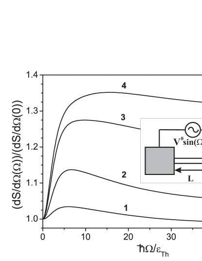
Figure 3: Frequency dependence of the differential photon-noise for a diffusive wire for given values of $A=eV^{o}/\hbar\Omega$. Here $\epsilon_{\rm Th}=\hbar D/L^{2}$ and the numerical calculation has been performed with 10 nodes. The magnitude of $dS/d\Omega$ is normalized to its value at $\Omega=0$. Curve (1) $A=1.0$, (2) $A=2.0$, (3) $A=3.0$, (4) $A=4.0$.

In conclusion, we have shown that the frequency dispersion of the photon assisted noise can be used to probe directly diffusion times in mesoscopic conductors. Our predictions can be verified by an experiment analogous to that described, for instance, in Ref. Reydellet et al. (2003), where a chaotic cavity or a diffusive wire should be substituted to the quantum point contact. By carefully choosing the transparencies of the cavity or the length of the wire, one can match the Thouless energy ($\hbar/\tau_{D}$) with the range of frequencies that have been already investigated. A Thouless energy of 10 $\mu$eV, that is typically realized in mesoscopic conductors, corresponds to $\Omega/2\pi=2.4$ GHz which is a frequency readily accessible in experiments.

We acknowledge useful discussions with F. Hekking, Yu. Nazarov, L. Levitov, and V. Vinokur. We acknowledge hospitality of Argonne National Laboratory where part of this work has been performed with support of the U.S. Department of Energy, Office of Science via the contract No. W-31-109-ENG-38. This work is also a part of research network of the Landesstiftung Baden-Württemberg gGmbH.

References

- Büttiker et al. (1993) M. Büttiker, A. Prêtre, and H. Thomas, Phys. Rev. Lett. 70, 4114 (1993).
- Naveh et al. (1999) Y. Naveh, D. V. Averin, and K. K. Likharev, Phys. Rev. B 59, 2848 (1999).
- Nagaev (1998) K. E. Nagaev, Phys. Rev. B 57, 4628 (1998).
- Golubev and Zaikin (2004) D. S. Golubev and A. D. Zaikin, Phys. Rev. B 69, 075318 (2004).
- Nagaev et al. (2004) K. E. Nagaev, S. Pilgram, and M. Büttiker, Phys. Rev. Lett. 92, 17804 (2004).
- Hekking and Pekola (2006) F. W. J. Hekking and J. P. Pekola, Phys. Rev. Lett. 96, 056603 (2006).
- Volkov et al. (1993) A. F. Volkov, A. V. Zaitsev, and T. M. Klapwijk, Physica C 210, 21 (1993).
- Hekking and Nazarov (1994) F. W. J. Hekking and Y. V. Nazarov, Phys. Rev. B 49, 6847 (1994).
- Belzig and Nazarov (2001) W. Belzig and Y. V. Nazarov, Phys. Rev. Lett. 87, 067006 (2001).
- Houzet and Pistolesi (2004) M. Houzet and F. Pistolesi, Phys. Rev. Lett. 92, 107004 (2004).
- Reulet and Prober (2005) B. Reulet and D. E. Prober, Phys. Rev. Lett. 95, 066602 (2005).
- Lesovik and Levitov (1994) G. B. Lesovik and L. S. Levitov, Phys. Rev. Lett. 72, 538 (1994).
- Schoelkopf et al. (1997) R. J. Schoelkopf, P. J. Burke, A. A. Kozhevnikov, D. E. Prober, and M. J. Rooks, Phys. Rev. Lett. 78, 3370 (1997).
- Reydellet et al. (2003) L.-H. Reydellet, P. Roche, D. C. Glattli, B. Etienne, and Y. Jin, Phys. Rev. Lett. 90, 176803 (2003).
- Rychkov et al. (2005) V. S. Rychkov, M. L. Polianski, and M. Büttiker, Phys. Rev. B 72, 155326 (2005).
- Polianski et al. (2005) M. L. Polianski, P. Samuelsson, and M. Büttiker, Phys. Rev. B 72, 161302 (2005).
- Altshuler et al. (1994) B. L. Altshuler, L. S. Levitov, and A. Y. Yakovets, JETP Letters 59, 857 (1994).
- Usadel (1970) K. D. Usadel, Phys. Rev. Lett. 25, 507 (1970).
- Larkin and Ovchinninkov (1986) A. I. Larkin and Y. V. Ovchinninkov, in Non equilibrium superconductivity, edited by D. Langenberg and A. I. Larkin (Elsevier, Amsterdam, 1986).
- Nazarov (1999a) Y. V. Nazarov, Superlattices Microstruct. 25, 1221 (1999a).
- Nazarov (1999b) Y. V. Nazarov, Ann. Phys. (Leipzig) 8, 193 (1999b).
- Levitov et al. (1996) L. S. Levitov, H. W. Lee, and G. B. Lesovik, J. Math. Phys. 37, 4845 (1996).
- Kamenev and Andreev (1999) A. Kamenev and A. Andreev, Phys. Rev. B 60, 2218 (1999).
- Shytov (2005) A. V. Shytov, Phys. Rev. B 71, 085301 (2005).
- Nazarov and Bagrets (2002) Y. V. Nazarov and D. A. Bagrets, Phys. Rev. Lett. 88, 196801 (2002).