Cooperative effect of load and disorder in thermally activated rupture of a $2d$ random fuse network

Abstract

A random fuse network, or equivalently a $2d$ spring network with quenched disorder, is submitted to a constant load and thermal noise, and studied by numerical simulations. Rupture is thermally activated and the lifetime follows an Arrhenius law where the energy barrier is reduced by disorder. Due to the non-homogenous distribution of forces from stress concentration at microcracks’ tips, spatial correlations between rupture events appear, but they do not affect the energy barrier’s dependence on disorder, they affect only the coupling between disorder and the applied load.

The effect of quenched disorder on dynamics is a recurring problem in many physical systems with elastic interactions. The motion of vortex lines in supraconductors, charge-density waves in Bragg glasses, magnetic domains walls, or contact lines in wetting show a competition between elastic interactions and pinning by disorder [1, 2]. While many studies have focused on systems driven above a critical depininng threshold, an important issue remains to understand the sub-critical regime, when thermally activated creep motion occurs [3, 4].

Rupture in disordered brittle solids falls in the same class of problems [5]. Elastic interactions tend to make a crack propagate in a straight direction while disorder creates roughness [6] or causes spatially diffuse damage [7, 8]. In the sub-critical rupture regime, a very important quantity for safety reasons is the lifetime, i.e. the mean time for a sample to break under a prescribed load. The lifetime follows an Arrehnius law [9, 10], but thermal noise is generally too small compared to recent theoretical estimates of the energy barrier [11, 12, 13] to explain experimental observations in heterogenous materials [14, 15, 16]. For athermal systems, disorder actually reduces the energy barrier and can be seen as an effective temperature [17]. In order to clarify the role of disorder in thermal systems, one-dimensional Thermal and Disordered Fiber Bundles Models ($1d$-TDFBM) have been introduced to model the thermally activated rupture of an heterogenous material submitted to a constant external load [18, 19, 20, 21, 22]. The TDFBM considers an elastic system in equilibrium at constant temperature where statistical force fluctuations occur in time due to thermal noise. This is very different from previous thermal random fuse models [23] where rupture results from an increase in fuse temperature due to dissipation through a generalized Joule effect until reaching a critical melting temperature. In a TDFBM, elastic energy is the equivalent of dissipation in the thermal random fuse model but does not cause rupture when the system is at mechanical equilibrium; rupture is caused by elastic force fluctuations analogous to Nyquist noise.

One problem with the $1d$-TDFBM investigated up to now is that the load is shared equally among all the unbroken fibers. This is not a realistic load-sharing rule for experimental geometries where elasticity cause stress concentration at microcracks’ tips and lead to a non-uniform redistribution of stress. In this letter, we show that spatial correlations between rupture events in $2d$ do not affect the dependence of the energy barrier on disorder but only the coupling between disorder and the applied load.

First, we discuss briefly results obtained by several authors [18, 19, 20, 21, 22] on the $1d$-TDFBM. The system considered is made of a set of $N$ parallel fibers, each carrying an initial force $f_{0}$ and behaving as a linear elastic spring with unity stiffness. Each fiber $j$ can carry a maximum force $f^{(j)}_{c}$ before it breaks. Quenched disorder is introduced in the system by distributing thresholds $f^{(j)}_{c}$ according to a gaussian distribution of mean $<f^{(j)}_{c}>=1$ and variance $T_{d}$; for each fiber, the value $f^{(j)}_{c}$ is a time-independent constant. Contrary to the case of non-thermal $1d$-DFBM where the system evolves due to a progressive increase in total current, we consider that the total force applied to the $1d$-TDFBM is kept constant. Dynamics is introduced in the system by introducing fluctuations in spring forces due to thermal noise. We write $f_{j}$ the average force on fiber $j$. The fluctuations in force $\delta f_{j}$ that occur in time on fiber $j$ are assumed to follow a gaussian probability distribution with $0$ mean value and variance $T$, where $T$ represents the thermodynamical temperature in unit of square force. When the total force on a fiber $f_{j}+\delta f_{j}$ is larger than the threshold $f^{(j)}_{c}$, the fiber breaks. The remaining fibers share equally the total force: this is a so-called democratic model. The bundle will break completely as soon as the average force on each fiber exceeds the breaking threshold. Roux has shown that the mean time to break the first fiber follows an Arrhenius law where disorder acts as an additive temperature [18]:

$$\tau\sim\exp\left(\frac{(1-f_{0})^{2}}{2(T+T_{d})}\right)$$ (1)

with $f_{0}$ the initial force carried by each fiber of the bundle. In the general case where many fibers break before total rupture of the bundle, the lifetime obeys an Arrhenius law with a different general form :

$$\tau\sim\exp\left(\frac{U(f_{0},T_{d})}{T}\right)$$ (2)

An approximate expression of $U$ for low disorder is [19, 20]:

$$U=\frac{1}{2}\left(1-f_{0}-\beta_{1}\sqrt{T_{d}}\right)^{2}$$ (3)

with $\beta_{1}=\sqrt{\pi/2}$. For higher disorder, Politi et al [21] have shown numerically that $U$ is determined with a very good approximation by the minimum value of the rate at which fibers break. More precisely, if $n$ is the number of broken fibers and $N$ the total number of fibers then $\Phi=n/N$ is the fraction of broken fibers and $\dot{\Phi}$ its time derivative. The value $\Phi^{*}$ for which $\dot{\Phi}$ is minimum obeys an implicit equation [21, 22]:

$$\exp\left[\rm{irfc}^{2}(2\Phi^{*})\right](1-\Phi^{*})^{2}=\alpha$$

where $\rm{irfc}$ is the inverse function of the complementary error function and $\alpha=f_{0}/\sqrt{2\pi T_{d}}$. Then, $U$ can be approximated as [24]:

$$U=\frac{1}{2}\left(1-f_{0}-\beta_{2}\sqrt{T_{d}}\right)^{2}\qquad\rm{with}\qquad\beta_{2}(\alpha)=\alpha\sqrt{2\pi}\frac{\Phi^{*}}{1-\Phi^{*}}+\sqrt{2}\,\rm{irfc}(2\Phi^{*})$$ (4)

Note that the coupling coefficient $\beta_{2}$ depends on both disorder $T_{d}$ and applied load $f_{0}$. Eq.(4) predicts that the variation of $U$ with $T_{d}$ for a fixed $f_{0}$ is non monotonous [22]. However, when $\alpha>1/4$ (this condition corresponds to $\Phi^{*}<1/2$ which would be expected in practice for most materials), $U$ decreases when $T_{d}$ is increased with $f_{0}$ constant. In that case, the function $\beta_{2}$ has a lower value $\beta_{2}(1/4)=\beta_{1}/2$ and an asymptotic behavior for large $\alpha$ ($\Phi^{*}\rightarrow 0$), $\beta_{2}(\alpha)\simeq\sqrt{2\ln\alpha}+1/\sqrt{2\ln\alpha}$ [21].

To study the effect of a non-uniform force redistribution on the rupture dynamics of the TDFBM, one could keep a $1d$ geometry and introduce a finite range of interaction between fibers [25]. Instead, we work directly in a $2d$ geometry more closely related to a real experiment. The above described 1d-TDFBM is equivalent to a system of parallel fuses where forces are transformed in currents and displacements in electric potentials. A $2d$ square fuse network is then equivalent to a square lattice of springs in antiplane deformation. Specifically, each node of the $N\times N$ nodes square lattice can move along an axis perpendicular to the plane of springs at rest. A constant force $F$ is applied at two opposite sides of the lattice in antiplane configuration. In the initial equilibrium configuration of the lattice, the springs submitted to a load $f_{0}=F/N$ are called ”parallel” springs while the unloaded springs (zero force) are called ”orthogonal” springs.

Like in $1d$, the fluctuations in force $\delta f_{j}$ on spring $j$ follow a gaussian probability distribution with $0$ mean value and variance $T$, and the rupture thresholds $f_{c}^{(j)}$ follow a gaussian distribution of mean $<f^{(j)}_{c}>=1$ and variance $T_{d}$. The time scale in the simulation is the (constant) time between two configurations of force fluctuations in the system. The whole network is a square with sides 100 springs wide; thus, the lattice contains about $2.\,10^{4}$ springs. Whenever we choose rupture thresholds from the gaussian distribution, there is a non-zero probability to obtain a negative threshold : $P_{<0}=\frac{1}{2}\rm{erfc}\left(<f_{c}>/\sqrt{2T_{d}}\right)$. For a system with $2\,10^{4}$ springs, we can safely consider that no spring will spontaneously break when there is no load ($f_{0}=0$) and at zero temperature if $P_{<0}<10^{-5}$, thus $T_{d}<0.055$ when $<f_{c}>=1$. In practice, we will work with $T_{d}<0.05$.

First, let us consider a lattice with no disorder in the rupture thresholds and all the springs initially intact. When thermal noise is on, some springs will start to break. Due to stress concentration effects, as soon as one of the parallel springs is broken, the neighboring springs are submitted to a larger force. If that new force exceeds the rupture threshold then the neighboring spring will also break, and the force on the next neighbor will be even higher. This process will result in the rupture of the whole network in an avalanche started from a single rupture event. Numerically, this will occur in our lattice as soon as $f_{0}>f_{c}^{1}$, where $f_{c}^{1}(\simeq 0.785)$ is the critical threshold of the homogenous lattice at $T=0$ when one parallel spring is broken. In that case, the rupture time will be directly related to the probability of breaking a single spring in the network and, if the lattice is disordered, we will recover essentially the result given by eq. (1) [18]. In the rest of the paper, we will be interested only in the case where several springs break before the final avalanche occurs, i.e. when $f_{0}<f_{c}^{1}$.

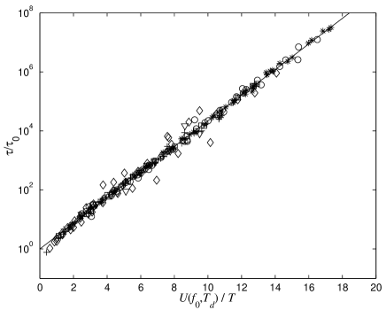
Figure 1: Scaled rupture time versus Arrhenius factor $U/T$. Various symbols correspond to different values of disorder and applied force. The solid line corresponds to $\log y=x$.

For a fixed value of the applied force $f_{0}$ and a fixed value of the disorder $T_{d}$, we measure as a function of temperature $T$ the lifetime, i.e. the rupture time averaged over as many as $100$ numerical experiments. We find that lifetime follows an Arrhenius law and obtain numerically $U(f_{0},T_{d})$ as defined by eq (2). We see on figure 1 the collapse of the data for a range of values $0.04<f_{0}<0.77$ and $10^{-4}<T_{d}<0.05$. Some of the data points are more scattered around the expected behavior (solid line) than others because the ratio of the standard deviation over the mean of the rupture time increases when $T$ becomes small. This property, already mentioned in [18], makes numerical convergence of the mean difficult in some cases.

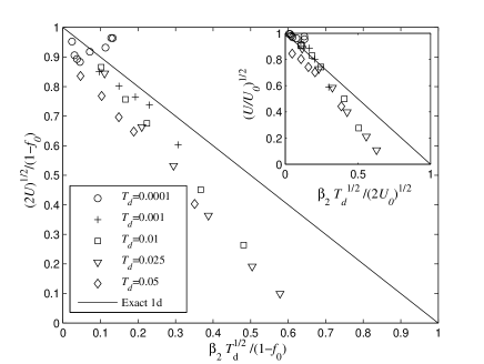
Figure 2: Comparison between the numerical value of $U$ in $2d$ and eq. (4) in $1d$ (solid line). Inset : same scaling, but using the numerical value $U_{0}=U(f_{0},0)$ for the $2d$ lattice.

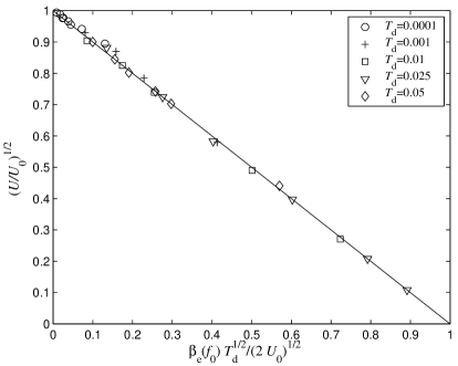
Figure 3: Collapse of all the numerical data using an effective value $\beta_{e}$ which is only a function of $f_{0}$ but not of $T_{d}$, contrary to the case of $\beta_{2}$ which is a function of $T_{d}$.

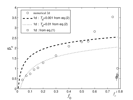
Figure 4: Numerical values of $\beta_{e}$ as a function of $f_{0}$ (circles). The dashed and dotted lines correspond to $\beta_{2}$ as predicted by eq. (4) when $T_{d}=0.001$ and $T_{d}=0.01$. Close to $f_{c}^{1}$, the values found for $\beta_{e}$ are close to values predicted by eq. (1).

To compare the barrier $U(f_{0},T_{d})$ for the $2d$ geometry with the one of the $1d$-TDFBM, we plot on figure 2 $\sqrt{2U}/(1-f_{0})$ as a function of $\beta_{2}\sqrt{T_{d}}/(1-f_{0})$. We clearly see that the functional form for $\beta_{2}$ is not correct, but also that the data for various values of disorder do not rescale very well. The first immediate reason for the discrepancy is that for $T_{d}=0$, the energy barrier of the $2d$ network $U_{0}=U(f_{0},0)$ (determined numerically) is not $(1-f_{0})^{2}/2$ as in $1d$. This is due to the preferential redistribution on the nearest neighbors of the force carried by a fiber before rupture. Taking into account the effective energy barrier in $2d$ does not improve the comparison with the 1d-TDFBM. After replacing $1-f_{0}$ by $\sqrt{2U_{0}}$ in eq. (4), we see in the inset of figure 2 that it is not enough to get a good collapse of all the data on the theoretical prediction (solid line).

We find that the barrier decreases with disorder following the linear curve : $\sqrt{U(f_{0},T_{d})}=\sqrt{U_{0}}-b\sqrt{T_{d}}$ for $10^{-4}<T_{d}<0.05$ and a fixed value of $f_{0}$. Thus, it turns out that eq. (3) is a much better functional form than eq. (4), even though it is an approximate expression in $1d$. Looking at eq. (3) or eq. (4), we can make an analogy with the $1d$ case and say that the second coefficient $b$ corresponds to an effective value $\beta_{e}/\sqrt{2}$ which is now only a function of $f_{0}$. On figure 3, we see the collapse of all the data when we plot $\sqrt{U/U_{0}}$ as a function of $\beta_{e}(f_{0})\sqrt{T_{d}}/\sqrt{2U_{0}}$.

The coupling coefficient $\beta_{e}$ increases almost linearly with $f_{0}$ up to values close to $f_{c}^{1}$ (figure 4). However, when $f_{0}$ gets very close to $f_{c}^{1}$, there is an abrupt decrease in the value of $\beta_{e}$. This is related to the fact that rupture is now controlled by a single event as in eq. (1). Indeed, although eq. (1) does not follow the general scaling property of eq.(2), we can estimate a value $\beta_{e}$ for each temperature value used in the simulation. The average value found for $\beta_{e}$ from eq. (1) (square symbols in figure 4 with an error bar corresponding to variations with temperature) is a reasonable estimate of the numerical value.

The functional behavior of $\beta_{e}$ is very different from that of the $1d$ model (eq. (4)) where $\beta_{2}$ depends on both $f_{0}$ and $T_{d}$. As an example, we plot on figure 4 $\beta_{2}(f_{0})$ for fixed values of $T_{d}$. Not only the functional dependence is clearly different from the numerical estimate $\beta_{e}(f_{0})$ but also $\beta_{2}$ decreases with $T_{d}$ at fixed $f_{0}$. In that sense, the load and the disorder do not act cooperatively in $1d$.

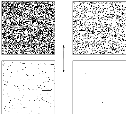
Figure 5: Image of the broken fibers (black dots) just before the final rupture for $T_{d}=0.01$ and $f_{0}=0.05$ (top left), $f_{0}=0.1$ (top right), $f_{0}=0.3$ (bottom left); $T_{d}=0.004$ and $f_{0}=0.75$ (bottom right). The arrow shows the loading direction.

The key point in $2d$ is that the spatial correlations between rupture events depend on the strength of stress intensification. This is illustrated on figure 5 a) to c) which shows the broken fibers just before the final avalanche for different values of $f_{0}$ and a fixed value of $T_{d}$. For very small loads, damage is scattered everywhere in the sample. At higher loads, damage becomes less scattered and growth of straight cracks occurs. Finally, figure 5d) shows that for a load close to the critical threshold, only very few events occur. A similar transition was observed for zero disorder or annealed disorder models with power law rate of rupture [26, 27, 28]. In contrast to these models where the transition occurs by changing the exponent of the power law, we observe a transition resulting from the competition between stress intensification and quenched disorder.

To understand this transition in our model, let us consider the increase in force due to stress intensification when a spring breaks. If the increase is small compared to $\sqrt{T_{d}}$, there will be very little spatial correlation between rupture events occurring preferentially at the weakest springs. For a given disorder, there is always a force $f_{0}$ small enough to observe this rupture regime similar to the $1d$-TDFBM case. On the contrary, if the increase due to stress intensification is large compared to $\sqrt{T_{d}}$, it is easier to break a spring next to an already broken spring, and the rupture will proceed mainly by growth of multiple cracks. In spite of very different regimes of spatial correlation between rupture events, we have the remarkable result that the energy barrier dependence on $T_{d}$ is unchanged. Spatial correlations only affects the coupling coefficient $\beta_{e}$, increasing quasi-linearly with $f_{0}$ and independent of $T_{d}$.

The multiplicative amplification of disorder due to $\beta_{e}$ is a mechanism that will create a load-dependent reduction of the energy barrier in thermally activated rupture. It will have an effect on the order of magnitude and load-dependence of the rupture time which could help understanding experiments in heterogeneous materials [14].

In conclusion, we have studied thermally activated rupture of a $2d$ elastic spring network submitted to a constant load and thermal noise. We find that spatial correlations between rupture events are controlled by a competition between quenched disorder and force inhomogeneities due to stress concentration. For low spatial correlations, the energy barrier scales naturally like in the $1d$ model. Remarkably, the appearance of spatial correlations does not affect the functional dependence of the energy barrier on disorder, but only the coupling coefficient $\beta_{e}$ which is independent of disorder and increases quasi-linearly with the applied load $f_{0}$. This is an important result showing that the applied load contribute to amplify in a cooperative way the effect of disorder on the lifetime. The observed cooperative effects of load and disorder in $2d$ subcritical rupture could be relevant to the creep regime of other physical systems with elastic interactions [1, 2] and also to crackling noise [29].

References

References

- [1] Kardar M. 1998 Phys. Rep. 301 85.
- [2] Chauve P., Giamarchi T. and Le Doussal P. 2000 Phys. Rev. B 62 6241.
- [3] Kolton A. B., Rosso A. and Giamarchi T. 2005 Phys. Rev. Lett. 94 047002; 95 180604.
- [4] Ogawa N., Miyano K. and Brazovski S. 2005 Phys. Rev. B 71 075118.
- [5] Ramanathan S. and Fisher D. S. 1998 Phys. Rev. B 58 6026.
- [6] Bouchaud E. 1997 J. Phys.: Condens. Matter 9 4319.
- [7] Herrmann H. J. and Roux S. (eds) 1990 Statistical Models for the Fracture of Disordered Media (Amsterdam, Elsevier).
- [8] Garcimartin A., Guarino A., Bellon L. and Ciliberto S. 1997 Phys. Rev. Lett. 79 3202.
- [9] Brenner S. S. 1962 J. Appl. Phys. 33 33.
- [10] Zhurkov S. N. 1965 Int. J. Fract. Mech. 1 311.
- [11] Golubovic L. and Feng S. 1991 Phys. Rev. A 43 5223.
- [12] Pomeau Y. 1992 C.R. Acad. Sci. Paris II 314 553.
- [13] Buchel A. and Sethna J. P. 1996 Phys. Rev. Lett. 77 1520.
- [14] Guarino A., Garcimartín A. and Ciliberto S. 1999 Europhys. Lett. 47 456.
- [15] Santucci S., Vanel L. and Ciliberto S. 2004 Phys. Rev. Lett. 93 095505.
- [16] Rabinovitch A., Friedman M. and Bahat S. 2004 Europhys. Lett. 67 969.
- [17] Arndt P. F. and Nattermann T. 2001 Phys. Rev. B 63 134204.
- [18] Roux S. 2000 Phys. Rev. E 62 6164.
- [19] Scorretti. R., Ciliberto. S. and Guarino A. 2001 Europhys. Lett. 55 (5) 626.
- [20] Ciliberto S., Guarino A. and Scorretti R. 2001 Physica D 158 83.
- [21] Politi A., Ciliberto S. and Scorretti R. 2002 Phys. Rev. E 66 026107.
- [22] Saichev A. and Sornette D. 2005 Phys. Rev. E 71 016608.
- [23] Sornette D. and Vanneste C. 1992 Phys. Rev. Lett. 68 612.
- [24] This is the correct expression of . It has been published with several typographic mistakes as eq. (35) in [22].
- [25] Yewande O. E. , Moreno Y., Kun. F., Hidalgo R. C. and Herrmann H. J. 2003 Phys. Rev. E 68 026116.
- [26] Hansen A., Roux S. and Hinrinchsen E. L. 1990 Europhys. Lett. 13 517.
- [27] Curtin W. A. and Scher H. 1997 Phys. Rev. B 55 12038.
- [28] Newman W. I. and Phoenix S. L. 2001 Phys. Rev. E 63 021507.
- [29] Sethna J. P., Dahmen K. A. and Myers C. R. 2001 Nature 10 242.