Interplay of paramagnetic, orbital and impurity effects on the phase transition of a normal metal to superconducting state

Abstract

We derive the generalized Ginzburg-Landau free energy functional for conventional and unconventional singlet superconductors in the presence of paramagnetic, orbital and impurity effects. Within the mean field theory, we determine the criterion for appearence of the non uniform (Fulde-Ferrell-Larkin-Ovchinnikov) superconducting state, with vortex lattice structure and additional modulation along the magnetic field. We also discuss the possible change of the order of transition from normal to superconducting state. We find that the superconducting phase diagram is very sensitive to geometrical effects such as the nature of the order parameter and the shape of the Fermi surface. In particular, we obtain the qualitative phase diagrams for three-dimensional isotropic s-wave superconductors and in quasi two-dimensional d-wave superconductors under magnetic field perpendicular to the conducting layers.

In addition, we determine the criterion for instability toward non uniform superconducting state in s-wave superconductors in the dirty limit.

I Introduction

The relative importance of orbital and paramagnetic effects in suppression of superconductivity is determined by the ratio of the orbital upper critical field Gor ; Wert $H_{c20}\approx\Phi_{0}/2\pi\xi_{0a}\xi_{0b}$ and the paramagnetic limiting field Clog ; Chandr $H_{p}=\Delta_{0}/\sqrt{2}\mu\approx 0.71\Delta_{0}/\mu$, called the Maki parameter Maki $\alpha_{M}=\sqrt{2}H_{c20}/H_{p}$. Here $\Phi_{0}$ is the flux quantum, $\xi_{0a}$ and $\xi_{0b}$ are the superconducting coherence lengths in two mutually perpendicular and perpendicular to magnetic field directions a and b, $\Delta_{0}$ is the superconducting gap at zero temperature and $\mu=g\mu_{B}/2$ is the electron magnetic moment. Usually, the Maki parameter is of the order of the ratio of critical temperature to the Fermi energy $\alpha_{M}\approx T_{c}/\varepsilon_{F}$. That demonstrates the negligibly small influence of paramagnetic effects on superconductivity. However, in the case of small Fermi velocity (that happens in materials with heavy electronic effective mass) or in the layered metals under magnetic field parallel to the layers, the value of the Maki parameter can be even larger than unity.

The consideration of the magnetic field acting only on the electron spins, corresponding to the limiting case of infinitely large Maki parameter, leads to some peculiar effects. First, the phase transition from the normal metal to the superconducting state which is of the second order in low field - high temperature region changes to the first order Sar ; MaTs ; Saint at fields above $H^{*}\approx 1.06T_{c}/\mu$ and temperatures below $T^{*}\approx 0.56T_{c}$. Starting at this critical point, the line of the first order transition is finished at zero temperature and at the magnetic field equal to the Chandrasekhar-Clogston limiting field $H_{p}$. However, as was shown by Fulde and Ferrell FF and Larkin and Ovchinnikov LO , even at larger field $H_{\text{FFLO}}\approx 0.755\Delta_{0}/\mu\approx 1.07H_{p}$, the normal state is unstable with respect to the second order type transition to the inhomogeneous cosine like gap modulated superconducting state (FFLO state) with wave vector $q_{c}\approx 2.38\mu H_{\text{FFLO}}/v_{F}$. The recent calculations Bow at zero temperature have demonstrated that more complicated crystal structures are more favorable than the simple plane wave. A first order type transition to the face-centered cube superconducting state was predicted to occur at the field larger than $H_{\text{FFLO}}$. This conclusion is in correspondence with the finite temperature investigations performed in vicinity of critical point showing the appearence of FFLO superconducting state below the critical temperature Buz ; Mora .

These results are changed a lot due to effects of orbital depairing and impurities.

The role of the orbital effects was studied first at $T=0$ by Gruenberg and Gunther Gru who have demonstrated that the FFLO state appears in pure metal (assuming that it is formed by means the second order transition) if the Maki parameter is larger than $1.8$.

The influence of impurities in absence of the orbital effect was investigated by Aslamazov Asl . He found that impurities do not kill the FFLO state but decrease the field $H_{\text{FFLO}}$ of absolute instability of the normal state for the FFLO formation such that, in the dirty limit ($\tau T_{c}\ll 1$), at zero temperature, $H_{\text{FFLO}}$ is lower than the field of the first order transition to homogeneous superconducting state, $H_{p}$. Physically, it does not yet abolish a possibility of existence of inhomogeneous superconducting state because the actual phase transition from the normal state could be of the first order transition to FFLO state at some field $H>H_{p}$ .

The investigation of orbital effects near the critical point was performed for isotropic three-dimensional pure metals by Houzet and Buzdin Houz . It was found that, unlike the conclusions obtained in the absence of orbital effect, for finite but large enough Maki parameter, the FFLO modulated state arises from the normal state starting from some temperature higher than the critical temperature.

All the studies cited above concerned the case of isotropic s-wave superconductivity. The theoretical interest to the FFLO state in superconductors with d-pairing MakiWon ; Sam ; Kun ; Vor was stimulated by the experimental identification of the pairing state in several of the high-$T_{c}$ cuprate superconductors and heavy fermionic materials.

The recently discovered heavy fermionic tetragonal compound $CeCoIn_{5}$ was established as $d_{x^{2}-y^{2}}$ superconductor similar to high-$T_{c}$ cuprates Mov ; Iza . In this compound, the phase transition to the superconducting state becomes of the first order at low temperature - high field region and possible formation of FFLO at lower temperatures was reported for the magnetic field directed parallel Bian02 ; Mic ; Bian03 as well as perpendicular Bian03 to the basal plane.

The first theoretical investigation of the phase diagram in the tetragonal, doped-by-impurities superconductor with d-pairing under the field parallel to c-axis was done in the Ref.Agt . It was found that, in the absence of orbital effect, the change of the type of transition from the second to the first order occurs at some temperature which is lower than the temperature of appearence of FFLO state.

The orbital effect in the same type of superconductor with quasi two-dimensional spectrum was taken into account by Ikeda and Adachi Ik and the different phase diagram topology was established. That is, in contrast with clean s-wave isotropic superconductor, the FFLO state arises from the normal state starting from some temperature lower than the critical temperature. This result was ascribed by the authors of Ref. Ik to the nonpertubative treatment of the orbital effects incorporated there.

It seems, however, that, in absence of analytical calculations, it is dificult to recognize an inequivocal reason for this discrepancy. The main goal of the present article is to make clear the influence of paramagnetic, orbital and impurity effects on the phase transition of a normal metal to superconducting state, including the FFLO state formation and type of the phase transition. With this purpose, we shall derive Ginzburg-Landau functional for the conventional and unconventional superconducting state with singlet pairing in the metal with arbitrary point symmetry and with arbitrary amount of point like (s-wave scattering) impurities. Then, for the cases of isotropic metal with s-pairing and tetragonal superconductor with d-pairing under magnetic field parallel to c-axis, the simple analytic criteria of appearence of FFLO state and the type of normal-superconductor phase transition shall be established. In particular, we shall demonstrate which temperature of FFLO appearence or the critical point temperature is higher.

The structure of the article is as follows. We begin with the general expressions of Ginzburg-Landau functional for the superconducting state (in metal with the arbitrary concentration of impurities) transforming according to identity and non-identity representations of the crystal point group symmetry. The corresponding derivation of this functional from microscopic theory valid at finite temperature in vicinity of critical point is found in the Appendices. Then, for the cases of s-pairing and d-pairing, the criteria of FFLO state existence and the first order type transition and their competition shall be formulated. In addition to these finite temperature calculations, the critical field of dirty normal metal instabilty to FFLO state formation in presence of the orbital effect (generalization of the papers by Gruenberg and Gunther Gru and by Aslamazov Asl ) at zero temperature is found.

II Free energy near critical point

The Ginzburg-Landau functional consists of the sum of the leading terms in the expansion of the superconducting free energy in the order parameter $\Delta$ and its gradients.

In the purely orbital limit, it contains terms proportional to $|\Delta|^{2}$, $|\Delta|^{4}$ and $|\nabla\Delta|^{2}$, with coefficients depending on the temperature and impurity concentration. Strictly speaking, it is only valid near the critical temperature $T_{c}$ of the second order transition from normal to superconducting state, when the coefficient $\alpha$ in front of $|\Delta|^{2}$ vanishes. Close to this point, the amplitude of the gap is indeed small and the magnetic length which determines the characteristic scale of the variation of $\Delta$ coincides with the thermal correlation length which diverges at $T_{c}$. This allows to retain only the first term in gradient expansion.

In the purely paramagnetic limit, the coefficients in the functional also depend on the magnetic field. The equation $\alpha(T,H)=0$ then defines the transition line $H_{0}(T)$ from normal state to uniform superconducting state in the temperature-magnetic field phase diagram. Along this line, the coefficient $\gamma$ in front of $|\nabla\Delta|^{2}$ happens to change its sign. This signals the instability toward the modulated FFLO superconducting state. In order to establish the modulation wavelength in FFLO state, higher order terms in the gradient expansion should also be included in the functional. One can restrict the free energy expansion to the term $|\nabla^{2}\Delta|^{2}$ only in the vicinity of the triple point, where the FFLO instability occurs and the typical FFLO modulation wavelength diverges. The coefficient $\beta$ in front of $|\Delta|^{4}$ also may change its sign. This signals a critical point when the type of the transition into uniform superconducting state changes from second order to first order as the temperature is lowered. In such case, the type of the transition into FFLO state will be determined by the sign of the fourth order terms in $\Delta$ and of higher order in the gradient expansion. Again, close to the critical point, one can consider the terms of the order $|\Delta|^{2}|\nabla\Delta|^{2}$ only Buz . The peculiarity of the microscopic theory is that, in the pure limit, $\gamma$ and $\beta$ change sign at the same place, with coinciding triple and critical point: the tricritical point $(T^{*},H^{*})$, with $H^{*}=H_{0}(T^{*})$. In the presence of impurities, however, the triple point and the critical point do not coincide any longer. For s-wave superconductors, the triple point occurs at lower temperature than the critical point, while for d-wave superconductors, the opposite situation takes place Agt .

The effect of the orbital field on the interplay between transition into conventional superconducting state (with vortex lattice in such case) and FFLO state (with FFLO modulation in the direction parallel to the vortex axes) was considered within this frame in s-wave superconductors and in pure limit only Houz . As it is important that the magnetic length remains large compared to the superconducting coherence length, a Ginzburg-Landau expansion is only possible when the paramagnetic effect is much larger than the orbital effect (large Maki parameter). In the pure s-wave superconductor, it was shown that the triple point was moved to higher temperatures Houz . Therefore, impurities and orbital effect act in opposite directions in the s-wave case.

The goal of the two next Sections is to provide a frame to discuss the nature of the transition from normal to superconducting state in the presence of impurities and a small orbital effect in superconductors with arbitrary (even and one-component) order parameter.

The free energy Ginzburg-Landau functional up to the fourth order terms of the order parameter and the fourth order terms in gradients for the isotropic s-pairing superconductors doped by impurities has been derived first in the paper Ovc . With a purpose of investigation of FFLO state in clean s-wave superconductors a similar result based on calculation using Eilenberger Eil and Larkin and Ovchinnikov LaOv formalism has been derived also in the paper Houz . The derivation for the dirty d-wave tetragonal superconductor based on the direct calculation of the vertex parts renormalization first introduced by Gor’kov Gor60 has been accomplished in the paper Agt , then including all orders in gradients in the paper Ik . Our derivation made for reliability by both Gor’kov Gor60 and Eilenberger Eil ; LaOv methods (see Appendices A and B) is related to the case of doped-by-impurities superconducting metal of arbitrary crystaline symmetry with an order parameter

$$\Delta(\hat{\bf k},{\bf r})=\psi(\hat{\bf k})\Delta({\bf r})$$ (1)

transformed according to either identity, $\langle\psi(\hat{\bf k})\rangle\neq 0$, or non-identity, $\langle\psi(\hat{\bf k})\rangle=0$, one-dimensional representation of the point group symmetry of the crystal Min . Here and after, the angular brackets mean the averaging over the Fermi surface, $\psi(\hat{\bf k})$ are the functions of irreducible representations, $\langle|\psi(\hat{\bf k})|^{2}\rangle=1$. The generalization for the multidimensional superconducting states can be easily considered.

The derivation for the case of superconducting state with an order parameter transforming according to general identity representation leads to quite cumbersome expression for the free energy. We shall consider the simplest example of identity representation with $\psi(\hat{\bf k})=1$, or s-wave pairing superconductivity, where the free energy functional is

$$F=\int d^{3}r\left\{\alpha|\Delta|^{2}+\pi N_{0}\Delta^{*}\left[\frac{K_{21}}{4}\langle({\bf v}{\bf D})^{2}\rangle\right.\right.$$

$$\left.-\left.\frac{K_{23}}{16}\langle({\bf v}{\bf D})^{4}\rangle-\frac{K_{33}}{32\tau}\langle({\bf v}{\bf D})^{2}\rangle^{2}\right]\Delta\right.$$

$$\left.+\pi N_{0}\frac{K_{30}}{4}|\Delta|^{4}\right.$$

$$\left.+\pi N_{0}\left(-\frac{K_{41}}{2}+\frac{K_{42}}{16\tau}\right)|\Delta|^{2}\langle({\bf v}{\bf D}\Delta)^{*}({\bf v}{\bf D}\Delta)\rangle\right.$$

$$\left.+\pi N_{0}\frac{K_{41}}{16}\left[(\Delta^{*})^{2}\langle({\bf v}{\bf D}\Delta)^{2}\rangle+c.c.\right]\right\}.$$ (2)

Here,

$$\alpha=N_{0}\Re\left[\Psi\left(\frac{1}{2}-\frac{i\mu H}{2\pi T}\right)-\Psi\left(\frac{1}{2}-\frac{i\mu H_{0}}{2\pi T}\right)\right]$$ (3)

and $H_{0}=H_{0}(T)$ is the critical field in homogeneous superconductor determined by the equation

$$\ln\frac{T_{c}}{T}=\Re\left[\Psi\left(\frac{1}{2}-\frac{i\mu H_{0}}{2\pi T}\right)-\Psi\left(\frac{1}{2}\right)\right].$$ (4)

The coefficients

$$K_{nm}=2T\Re{\sum^{\infty}}_{\nu=o}\frac{1}{(\omega_{\nu}-i\mu H)^{n}(\tilde{\omega}_{\nu}-i\mu H)^{m}},$$ (5)

and $\omega_{\nu}=\pi T(2\nu+1)$ are Matsubara frequencies,

$$\tilde{\omega}_{\nu}=\omega_{\nu}+\frac{\text{sign}~{}\omega_{\nu}}{2\tau},$$

${\bf D}=-i\nabla+(2\pi/\Phi_{0}){\bf A}$, ${\bf v}(\hat{\bf k})$ is the Fermi velocity, $N_{0}$ is the density of states at the Fermi level. We put through the article $\hbar=1$.

Near the critical temperature $T_{c}$, both fields $H_{0}(T)$ and the upper critical field tend to zero and the latter should be determined from the linear Ginzburg-Landau equation giving well known Gor’kov result Gor60 with small correction due to paramagnetic effect. On the contrary, near the tricritical point, at large enough Maki parameter the upper critical field is close to $H_{0}(T)$ such that one can write

$$\alpha = \alpha_{0}(H-H_{0})$$ (6)

$$= \frac{N_{0}\mu(H-H_{0})}{2\pi T}\Im\Psi^{\prime}\left(\frac{1}{2}-\frac{i\mu H_{0}}{2\pi T}\right)$$

and put $H=H_{0}$ in all other terms of the functional.

The free energy functional for non-identity representation is

$$F=\int d^{3}r\left\{\tilde{\alpha}|\Delta|^{2}\right.$$

$$+\left.\pi N_{0}\Delta^{*}\left[\frac{K_{03}}{4}\langle|\psi(\hat{\bf k})|^{2}({\bf v}{\bf D})^{2}\rangle\right.\right.$$

$$\left.-\left.\frac{K_{05}}{16}\langle|\psi(\hat{\bf k})|^{2}({\bf v}{\bf D})^{4}\rangle\right.\right.$$

$$\left.-\frac{K_{15}}{32\tau}\langle\psi(\hat{\bf k})^{*}({\bf v}{\bf D})^{2}\rangle\langle\psi(\hat{\bf k})({\bf v}{\bf D})^{2}\rangle\right]\Delta$$

$$\left.+\pi N_{0}\left(\frac{K_{03}}{4}\langle|\psi(\hat{\bf k})|^{4}\rangle-\frac{K_{04}}{8\tau}\right)|\Delta|^{4}\right.$$

$$\left.-\pi N_{0}\frac{K_{05}}{2}|\Delta|^{2}\langle|\psi(\hat{\bf k})|^{4}({\bf v}{\bf D}\Delta)^{*}({\bf v}{\bf D}\Delta)\rangle\right.$$

$$\left.+\pi N_{0}\frac{5K_{06}}{16\tau}|\Delta|^{2}\langle|\psi(\hat{\bf k})|^{2}({\bf v}{\bf D}\Delta)^{*}({\bf v}{\bf D}\Delta)\rangle\right.$$

$$\left.+\pi N_{0}\frac{K_{05}}{16}\left[(\Delta^{*})^{2}\langle|\psi(\hat{\bf k})|^{4}({\bf v}{\bf D}\Delta)^{2}\rangle+c.c.\right]\right.$$

$$\left.-\pi N_{0}\frac{K_{06}}{16\tau}\left[(\Delta^{*})^{2}\langle|\psi(\hat{\bf k})|^{2}({\bf v}{\bf D}\Delta)^{2}\rangle+c.c.\right]\right\}.$$ (7)

Here,

$$\tilde{\alpha}=N_{0}\Re\left[\Psi\left(\frac{1}{2}-\frac{i\mu H}{2\pi T}+\frac{1}{4\pi\tau T}\right)\right.$$

$$\left.-\Psi\left(\frac{1}{2}-\frac{i\mu\tilde{H}_{0}}{2\pi T}+\frac{1}{4\pi\tau T}\right)\right]$$ (8)

and $\tilde{H}_{0}=\tilde{H}_{0}(T)$ is the critical field in homogeneous superconductor determined by the equation

$$\ln\frac{T_{c}}{T}=\Re\left[\Psi\left(\frac{1}{2}-\frac{i\mu\tilde{H}_{0}}{2\pi T}+\frac{1}{4\pi\tau T}\right)-\Psi\left(\frac{1}{2}\right)\right].$$ (9)

Near the critical temperature $T_{c}$, both fields $\tilde{H}_{0}(T)$ and the upper critical field tend to zero and the latter should be determined from the linear Ginzburg-Landau equation. Near the tricritical point, at large enough Maki parameter, the upper critical field is close to $\tilde{H}_{0}(T)$ such that one can write

$$\tilde{\alpha} = \tilde{\alpha}_{0}(H-\tilde{H}_{0})$$ (10)

$$= \frac{N_{0}\mu(H-\tilde{H}_{0})}{2\pi T}\Im\Psi^{\prime}\left(\frac{1}{2}-\frac{i\mu\tilde{H}_{0}}{2\pi T}+\frac{1}{4\pi\tau T}\right)$$

and put $H=\tilde{H}_{0}$ in all other terms of the functional.

In addition to the superconducting energy (2) or (7), one should in principle also include the magnetic energy

$$F_{m}=\frac{1}{8\pi}\int d^{3}r({\bf H-H_{\text{ext}}})^{2},$$ (11)

where $\bf H_{\text{ext}}$ is the external field, in the total free energy functional. In the following, we will negelect the contribution of such term by assuming that the screening current are not important (high-$\kappa$ limit) and $\bf H=H_{\text{ext}}$.

III Criteria for the appearence of FFLO state and the first order transition

III.1 Identity representation

With the purpose to derive simple analytic criteria for the appearence of FFLO state and the change of the second order normal metal - superconductor transition to the first order one, let us make the angular averaging in the expression (2) for the free energy in the case of pure s-pairing ($\psi(\hat{\bf k})=1$) in a metal with spherical Fermi suface:

$$F=\int d^{3}r\left\{\alpha_{0}(H-H_{0})|\Delta|^{2}+\frac{\pi N_{0}v^{2}K_{21}}{12}\Delta^{*}({\bf D})^{2}\Delta\right.$$

$$\left.-\frac{\pi N_{0}v^{4}K_{23}}{80}\Delta^{*}\left(({\bf D}^{2})^{2}+\frac{1}{\lambda^{4}}\right)\Delta\right.$$

$$\left.-\frac{\pi N_{0}v^{4}K_{33}}{288\tau}\Delta^{*}({\bf D}^{2})^{2}\Delta+\frac{\pi N_{0}K_{30}}{4}|\Delta|^{4}\right.$$

$$\left.+\pi N_{0}v^{2}\left(-\frac{K_{41}}{6}+\frac{K_{42}}{48\tau}\right)|\Delta|^{2}|{\bf D}\Delta|^{2}\right.$$

$$\left.+\frac{\pi N_{0}v^{2}K_{41}}{48}\left[(\Delta^{*})^{2}({\bf D}\Delta)^{2}+c.c.\right]\right\},$$ (12)

where $v$ is the modulus of Fermi velocity and the term $\lambda^{-4}=(2eH/c)^{2}$ originates from noncommutativity of the operators $D_{x}$ and $D_{y}$. This value serves as the measure of the orbital effect such that the orbital effects free situation corresponds to the limit $\lambda\to\infty$.

Let us choose the magnetic field direction along the z-axis ${\bf A}=(0,Hx,0))$. So, for the Abrikosov lattice ground state $\Delta=\varphi_{0}(x,y)f(z)$ which is the linear combination of Landau wave fuctions with $n=0$ multiplied by exponentially $f_{\text{exp}}=\exp(iqz)$ or sinusoidally $f_{\text{sin}}=\sqrt{2}\sin qz$ modulated function along z-direction, one can substitute

$${\bf D}^{2}\Delta=({\bf D}_{\perp}^{2}+D_{z}^{2})\Delta=\left(\frac{1}{\lambda^{2}}+q^{2}\right)\Delta.$$ (13)

Making use of the properties:

$$({\bf D}_{\perp}\Delta)^{2}=0,~{}~{}~{}\int d^{3}r|\Delta|^{2}|{\bf D}_{\perp}\Delta|^{2}=\frac{1}{2\lambda^{2}}\int d^{3}r|\Delta|^{4},$$ (14)

we come to the free energy in the following form

$$F=\int dxdy\left\{\alpha_{0}\left(H-H(q)\right)|\varphi_{0}|^{2}+\pi N_{0}B|\varphi_{0}|^{4}\right\},$$ (15)

where

$$H(q)=H_{0}-\frac{\pi N_{0}}{\alpha_{0}}\left[\frac{v^{2}K_{21}}{12}\left(\frac{1}{\lambda^{2}}+q^{2}\right)\right.$$ (16)

$$\left.-\frac{v^{4}K_{23}}{80}\left(\left(\frac{1}{\lambda^{2}}+q^{2}\right)^{2}+\frac{1}{\lambda^{4}}\right)\right.\left.-\frac{v^{4}K_{33}}{288\tau}\left(\frac{1}{\lambda^{2}}+q^{2}\right)^{2}\right],$$

and the coefficient $B$ is given by

$$B_{0}=\frac{K_{30}}{4}-\frac{v^{2}}{2\lambda^{2}}\left(\frac{K_{41}}{6}-\frac{K_{42}}{48\tau}\right)$$ (17)

in the conventional superconducting vortex-lattice state,

$$B_{\text{exp}}=B_{0}-v^{2}q^{2}\left(\frac{K_{41}}{8}-\frac{K_{42}}{48\tau}\right)$$ (18)

in the exponentially modulated FFLO phase, and

$$B_{\text{sin}}=\frac{3B_{0}}{2}-\frac{q^{2}v^{2}}{2}\left(\frac{5K_{41}}{24}-\frac{K_{42}}{48\tau}\right)$$ (19)

in the sinusoidally modulated FFLO phase.

The critical field value $H_{c}$ is found by taking the maximum of $H=H(q)$ as the function of $q$. The usual superconducting state appears at $q=0$, while the FFLO state is formed when the maximum of $H$ is reached at finite $q=q_{0}$, where

$$q_{0}^{2}=-\frac{1}{\lambda^{2}}+\frac{\frac{K_{21}}{3v^{2}}}{\frac{K_{23}}{10}+\frac{K_{33}}{36\tau}}.$$ (20)

The FFLO state appears when the coefficient at $q^{2}$ in the square brackets of Eq. (16) changes the sign from positive to negative and it exists at

$$K_{21}~{}<~{}\frac{3v^{2}}{\lambda^{2}}\left(\frac{K_{23}}{10}+\frac{K_{33}}{36\tau}\right).$$ (21)

Let us now examine the question of the transition type. It is determined by the sign of the coefficient at $|\varphi_{0}|^{4}$ in the expression (15) for the free energy. Hence, the first order transition occurs at $B_{0}<0$ for the transition into usual superconducting state. It occurs at $B_{\text{exp}}(q_{0})<0$ for transition into FFLO state with exponential modulation or $B_{\text{sin}}(q_{0})<0$ for transition into FFLO state with sinusoidal modulation.

To see explicitly the role of orbital effects and the impurities in the formation of FFLO state and the change of the transition type, let us look on them separetely.

In the clean, paramagnetic limit ($\lambda,\tau=\infty$), Eq. (15) coincides with the free energy derived in Ref. Buz . There, the inequality $K_{30}<0$ was obtained as the condition both for the change of the transition type from normal to uniform superconducting state and for the FFLO state formation. In the vicinity of the tricritical point, keeping $H=H_{0}(T)$ in $K_{30}$, one finds that $K_{30}$ changes its sign as a function of the temperature when $T=T^{*}$. Therefore, $K_{30}\propto(T-T^{*})$ has the meaning of an effective temperature close to this point. Further study reveals that, while $B_{\text{exp}}(q_{0})=-K_{30}/6$ remains positive at $T<T_{t}$, $B_{\text{sin}}(q_{0})=K_{30}/36$ becomes negative. This means that the first order transition from sinusoidally modulated FFLO state is favored at $T<T^{*}$. The qualitative superconducting phase diagram which results from this study is shown on Fig. 1(a).

Figure 1: Qualitative superconducting phase diagram for three-dimensional s-wave superconductor in presence of strong paramagnetic effect. The clean, purely paramagnetic case is shown on (a), the purely paramagnetic case with disorder is shown on (b), and the clean case, with some orbital effect is shown on (c). Possible phases are the normal state (N), the conventional superconducting state: uniform state (U) in the absence or orbital effect, Abrikosov vortex lattice state (A) in presence of orbital effect, and the FFLO modulated state with exponential modulation (FF) or sinusoidal modulation (LO) along the applied field, eventually with Abrikosov vortex lattice (A+FF or A+LO) if orbital effect is present. Thin lines correspond to second order transitions, thick lines correspond to first order transitions, dashed lines correspond to transitions between different superconducting states and they have not been calculated in the present work.

In presence of impurities but neglecting the orbital effect ($\lambda\to\infty$), we obtain from Eq. (21) inequality $K_{21}<0$ as condition of FFLO formation. It is easy to check that at the temperature determined by equation $K_{21}=0$, where the coefficient $K_{21}$ changes the sign and, hence, the finite $q$ modulation appears, the coefficient $K_{30}$ is already negative. Therefore, $B_{0}$ is negative and the normal metal transforms to homogeneous superconducting state by means of the first order transition. The impurities shift FFLO state to lower temperatures leaving unchanged the temperature of change of type of transition. The qualitative phase diagram in this limit is shown on Fig. 1(b).

On the other hand, taking into account only orbital effects, that is in the completely pure case ($\tau\to\infty$), one can rewrite the condition (21) of FFLO appearence as

$$K_{30}~{}<~{}\frac{3}{10}\frac{v^{2}K_{50}}{\lambda^{2}}.$$ (22)

In pure case and at $\lambda\to\infty$, the FFLO state appears exactly when the coefficient $K_{30}$ changes its sign. Whereas in presence of orbital effect, the FFLO state appears at slightly negative $K_{30}$ determined by negative value of $K_{50}$. Moreover, the condition of the first order transition into usual superconducting state, $B_{0}<0$, is rewritten as

$$K_{30}~{}<~{}\frac{1}{3}\frac{v^{2}K_{50}}{\lambda^{2}}$$ (23)

The comparison of these two inequalities makes clear that, due to the orbital effect, the change of the type of transition always appears at lower temperature than the FFLO state formation. This conclusion is in correspondence with the results of the paper Houz where the qualitative phase diagram shown on Fig. 1(c) was first proposed.

Thus, we find that impurities and orbital effect act in opposite directions regarding the shift of the temperature below which FFLO state will appear. In the following, we study the interplay between low impurities and orbital effect ($1/\lambda,1/\tau\rightarrow 0$) on FFLO state formation. In this limit, the change of the transition type at the normal/conventional superconducting vortex lattice transition, determined by $B_{0}<0$, is still given by Eq. (23). The temperature below which transition into FFLO state occurs is determined by Eq. (21). In leading order in $1/\lambda^{2}$ and $1/\tau$, this equation yields:

$$K_{30}<\frac{1}{2}\frac{K_{40}}{\tau}+\frac{3}{10}\frac{v^{2}K_{50}}{\lambda^{2}},$$ (24)

where we made use of the property :

$$K_{nm}\simeq K_{n+m,0}-\frac{m}{2\tau}K_{n+m+1,0}.$$

In Eqs. (23), (24), we recall that $K_{30}\propto(T-T^{*})$ has the meaning of an effective temperature, while $K_{40}$ and $K_{50}$ have to be evaluated at the tricritical point $(T^{*},H^{*})$, where they take negative values. By comparing Eqs. (23),(24), we find that the FFLO state appears at temperatures higher than the critical temperature when the impurity concentration remains low enough:

$$\frac{1}{\tau}<\frac{v^{2}}{15\lambda^{2}}\frac{K_{50}}{K_{40}}.$$ (25)

When Eq. (25) is obeyed, the free energy (15) also allows to discuss the structure of the FFLO state which is realized at the second order normal/FFLO transition. When $B_{\text{exp}}(q_{0})<B_{\text{sin}}(q_{0})$ (and both of them positive), with $q_{0}$ given by Eq. (20), the FFLO state with exponential modulation is energetically favored. In the limit of low impurity and orbital effect that we consider, this inequality corresponds to:

$$K_{30}>\frac{5}{28}\frac{K_{40}}{\tau}+\frac{9}{28}\frac{v^{2}K_{50}}{\lambda^{2}}.$$ (26)

The FFLO state with sinusoidal modulation is favored when $B_{\text{sin}}(q_{0})<B_{\text{exp}}(q_{0})$. The transition into this state becomes of the first order when $B_{\text{sin}}(q_{0})<0$, that is:

$$K_{30}<-\frac{25}{4}\frac{K_{40}}{\tau}+\frac{3}{4}\frac{v^{2}K_{50}}{\lambda^{2}}.$$ (27)

The above discussion is summarized on Fig. 2. It represents the nature and type of the transition from normal to the different superconducting states as temperature is lowered, for a given ratio between orbital and impurity effects.

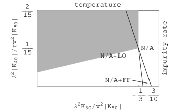
Figure 2: This figure shows the nature of the superconducting state which is realized just below the upper critical line, as well as the type of the transition, for three-dimensional s-wave superconductors with spherical Fermi surface, at large paramagnetic, small orbital and impurity effects, and for temperatures close to the tricritical temperature $T^{*}$. $\lambda^{2}K_{30}/v^{2}|K_{50}|\propto(T-T^{*})$ is the effective temperature, $\lambda^{2}|K_{40}|/\tau v^{2}|K_{50}|\propto\tau^{-1}$ is the ratio between orbital and impurity effects. N/A indicates the place where the transition is from normal state into conventional Abrikosov superconducting vortex lattice state, N/A+FF indicates the place where the transition is from normal state into FFLO state with vortex structure in the plane parpendicular to the magnetic field and exponential modulation along the field, N/A+LO indicates the place where the transition is into FFLO state with vortex structure in the plane perpendicular to the magnetic field and sinusoidal modulation along the field; in the white (gray) region, the transition into superconducting state is of the second (first) order.

When the transition is of the second order, minimization of the free energy (15) on $\varphi_{0}$ yields that the vortex lattice is triangular.Abrikosov

In the Ref.BuzBris , it was predicted that a very large Maki parameter may favor not only FFLO modulation, but also an order parameter formed of higher-level Landau functions: $\Delta\sim\varphi_{n}(x,y)f(z)$, with $n>0$. In Eqs. (14),(16) the expression $(\lambda^{-2}+q^{2})$ should be then replaced by $((2n+1)/\lambda^{2}+q^{2})$, and the fourth order term $B$ in the free energy (13) should also be calculated accordingly. In particular, the condition to maximize the critical field (16) at the second order transition from normal to vortex lattice state with Landau functions of level $n\geq 1$ is:

$$K_{30}<\frac{1}{2}\frac{K_{40}}{\tau}+\frac{3(2n+1)}{10}\frac{v^{2}K_{50}}{\lambda^{2}}.$$ (28)

This equation is obtained by requiring that $q_{0}^{2}>0$ in Eq. (20) after substituting $1/\lambda^{2}$ by $(2n+1)/\lambda^{2}$. One can note that, when such inequality is obeyed, the transition from normal to vortex lattice state (with $n=0$) has already turned from second to first order, both in the ”low impurity” case in the presence of sinusoidal modulation (because Eq. (27) is already obeyed), and in the ”high impurity” case (because Eq. (23) is already obeyed).

Therefore, we get now the qualitative picture of the superconducting phase diagram in three-dimensional s-wave superconductors with strong paramagnetic effect. At large impurity concentration, the transition from normal to usual superconducting state becomes of the first order at low temperatures, while FFLO state may exist at even more lower temperatures either as stable or as metastable state. On the other hand, at low impurity concentration, while temperature is lowered, the phase diagram shows the second order transition from normal to usual supercondutcing state, then to exponential FFLO state, then to sinusoidal FFLO state, and finally the change of the transition order into such state. These conclusions are summarized in the phase diagrams shown in Fig. 1 and 2.

III.2 Non-identity representation

As an example of similar calculations for nonconventional superconductivity we consider the d-wave superconducting state $\psi(\hat{\bf k})\propto k_{x}^{2}-k_{y}^{2}$ in tetragonal crystal under magnetic field along c-axis ($\hat{z}$-direction). One can rewrite first the Eq.  (7) in the following form

$$F=\int d^{3}r\left\{\tilde{\alpha}|\Delta|^{2}\right.$$

$$+\left.\pi N_{0}\Delta^{*}\left[\frac{K_{03}}{4}(\langle|\psi|^{2}v_{\perp}^{2}/2\rangle{\bf D}_{\perp}^{2}+\langle|\psi|^{2}v_{z}^{2}\rangle D_{z}^{2})\right.\right.$$

$$\left.\left.-\frac{K_{05}}{16}(\langle|\psi|^{2}({\bf v}{\bf D}_{\perp})^{4}\rangle+3\langle|\psi|^{2}v_{\perp}^{2}v_{z}^{2}\rangle{\bf D}_{\perp}^{2}D_{z}^{2}\right.\right.$$

$$\left.\left.+\langle|\psi|^{2}v_{z}^{4}\rangle D_{z}^{4})\right.\right.$$

$$\left.\left.-\frac{K_{15}}{32\tau}|\langle\psi\hat{v}_{\perp}^{2}/2\rangle{\bf D}_{\perp}^{2}+\langle\psi\hat{v}_{z}^{2}\rangle D_{z}^{2}|^{2}\right]\Delta\right.$$

$$\left.+\pi N_{0}\left(\frac{K_{03}}{4}\langle|\psi|^{4}\rangle-\frac{K_{04}}{8\tau}\right)|\Delta|^{4}\right.$$

$$\left.-\pi N_{0}\frac{K_{05}}{2}|\Delta|^{2}\left[\langle|\psi|^{4}v_{\perp}^{2}/2\rangle({\bf D}_{\perp}\Delta)^{*}{\bf D}_{\perp}\Delta\right.\right.$$

$$\left.\left.+\langle|\psi|^{4}v_{z}^{2}\rangle(D_{z}\Delta)^{*}D_{z}\Delta\right]\right.$$

$$\left.+\pi N_{0}\frac{5K_{06}}{16\tau}|\Delta|^{2}\left[\langle|\psi|^{2}v_{\perp}^{2}/2\rangle({\bf D}_{\perp}\Delta)^{*}{\bf D}_{\perp}\Delta\right.\right.$$

$$\left.\left.+\langle|\psi|^{2}v_{z}^{2}\rangle(D_{z}\Delta)^{*}D_{z}\Delta\right]\right.$$

$$\left.+\pi N_{0}\frac{K_{05}}{16}\left[(\Delta^{*})^{2}(\langle|\psi|^{4}v_{\perp}^{2}/2\rangle({\bf D}_{\perp}\Delta)^{2}\right.\right.$$

$$\left.\left.+(\Delta^{*})^{2}\langle|\psi|^{4}v_{z}^{2}\rangle(D_{z}\Delta)^{2})+c.c.\right]\right.$$

$$\left.-\pi N_{0}\frac{K_{06}}{16\tau}\left[(\Delta^{*})^{2}(\langle|\psi|^{2}v_{\perp}^{2}/2\rangle({\bf D}_{\perp}\Delta)^{2}\right.\right.$$

$$\left.\left.+(\Delta^{*})^{2}\langle|\psi|^{2}v_{z}^{2}\rangle(D_{z}\Delta)^{2})+c.c.\right]\right\}.$$ (29)

From this step, unlike to the conventional superconductivity, the continuation of calculation for d-pairing in closed analytical form is not possible. The point is that the average $\langle|\psi|^{2}({\bf v}{\bf D}_{\perp})^{4}\rangle=\langle|\psi|^{2}(D^{+}v^{-}+D^{-}v^{+})^{4}\rangle$ contains the terms $\langle|\psi|^{2}(D^{\pm}v^{\mp})^{4}\rangle$ which are not equal to zero in tetragonal crystal. Here $D^{\pm}=(D_{x}\pm iD_{y})/\sqrt{2}$, $v^{\pm}=(v_{x}\pm iv_{y})/\sqrt{2}$ and $v_{\perp}^{2}=v_{x}^{2}+v_{y}^{2}$. Hence, unlike to conventional superconductivity, the Abrikosov lattice ground state in tetragonal superconductor with d-pairing Vav is the linear combination of functions consisting of infinite series of Landau wave functions $\varphi_{n}(x,y)$ with n=0, 4, 8, 12…multiplied by exponentially or sinusoidally modulated function $f(z)$ along z-direction

$$\Delta=f(z)(A_{0}\varphi_{0}+A_{4}\varphi_{4}+A_{8}\varphi_{8}\ldots.)$$ (30)

Fortunately, in the limit of large Maki parameters we are interested in, one can work with cut-off series of the form similar to s-wave pairing

$$\Delta\approx f(z)\varphi_{0}$$ (31)

and also neglect the terms like $\langle|\psi|^{2}(D^{\pm}v^{\mp})^{4}\rangle$ in the Hamiltonian (the proof of this property is found in Appendix C). So, we shall use the substitution

$$\langle|\psi|^{2}({\bf v}{\bf D}_{\perp})^{4}\rangle\Delta$$

$$\Rightarrow~{}~{}\langle|\psi|^{2}(v^{-}v^{+})^{2}\rangle(D^{-}D^{+}D^{-}D^{+}+D^{-}D^{-}D^{+}D^{+})\Delta$$

$$=3\langle|\psi|^{2}(v^{-}v^{+})^{2}\rangle\lambda^{-4}\Delta$$ (32)

Thus, the further calculations have the sence of variational treatment.

Similar to the case of conventional superconductivity, we now obtain from Eq.  (29)

$$F=\int dxdy\left\{\tilde{\alpha}_{0}\left(H-\tilde{H}(q)\right)|\varphi_{0}|^{2}+\pi N(0)\tilde{B}|\varphi_{0}|^{4}\right\},$$ (33)

where

$$\tilde{H}(q)=\tilde{H}_{0}-\frac{\pi N_{0}}{\tilde{\alpha}_{0}}\left[\frac{K_{03}}{4}(\langle|\psi|^{2}v_{\perp}^{2}\rangle\frac{1}{2\lambda^{2}}+\langle|\psi|^{2}v_{z}^{2}\rangle q^{2})\right.$$

$$\left.-\frac{K_{05}}{16}(\frac{3}{4\lambda^{4}}\langle|\psi|^{2}v_{\perp}^{4}\rangle+\frac{3q^{2}}{\lambda^{2}}\langle|\psi|^{2}v_{\perp}^{2}v_{z}^{2}\rangle+\langle|\psi|^{2}v_{z}^{4}\rangle q^{4})\right.$$

$$\left.-\frac{K_{15}}{32\tau}|\langle\psi v_{\perp}^{2}\rangle\frac{1}{2\lambda^{2}}+\langle\psi v_{z}^{2}\rangle q^{2}|^{2}\right]$$ (34)

and

$$\tilde{B}_{0}=\frac{K_{03}}{4}\langle|\psi|^{4}\rangle-\frac{K_{04}}{8\tau}-\frac{K_{05}}{8\lambda^{2}}\langle|\psi|^{4}v_{\perp}^{2}\rangle+\frac{5K_{06}}{64\tau\lambda^{2}}\langle|\psi|^{2}v_{\perp}^{2}\rangle$$ (35)

for the conventional superconducting vortex lattice state,

$$\tilde{B}_{\text{exp}}(q)=\tilde{B}_{0}+q^{2}\left(-\frac{3K_{05}}{8}\langle|\psi|^{4}v_{z}^{2}\rangle+\frac{3K_{06}}{16\tau}\langle|\psi|^{2}v_{z}^{2}\rangle\right)$$ (36)

for the exponentially modulated FFLO state, and

$$\tilde{B}_{\text{sin}}(q)=\frac{3\tilde{B}_{0}}{2}+\frac{q^{2}}{2}\left(-\frac{5K_{05}}{8}\langle|\psi|^{4}v_{z}^{2}\rangle+\frac{7K_{06}}{16\tau}\langle|\psi|^{2}v_{z}^{2}\rangle\right)$$ (37)

for the sinusoidally modulated FFLO state.

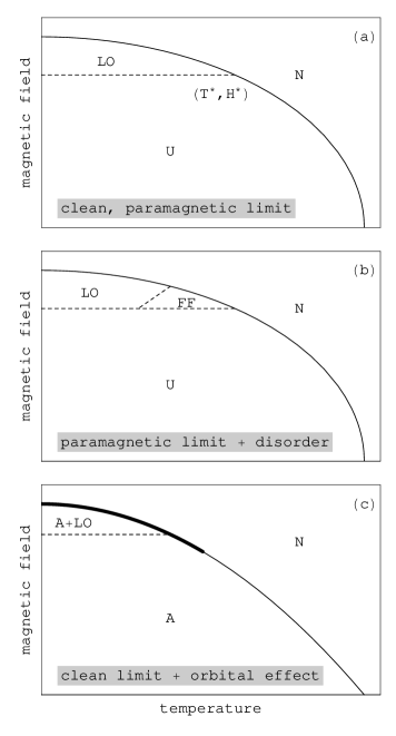
Figure 3: Qualitative superconducting phase diagram for quasi two-dimensional d-wave superconductor in presence of strong paramagnetic effect. (see also legend of Fig. 1).

The study is now similar to the previous section.

The critical field $H_{c}$ is determined by the maximum of $\tilde{H}(q)$ as the function of $q$. The FFLO state arises when the maximum of $H$ occurs at finite wave vector

$$q_{0}^{2}=$$ (38)

$$\frac{K_{03}\langle|\psi|^{2}v_{z}^{2}\rangle-\frac{3K_{05}\langle|\psi|^{2}v_{\perp}^{2}v_{z}^{2}\rangle}{4\lambda^{2}}-\frac{K_{15}\Re(\langle\psi^{*}v_{\perp}^{2}\rangle\langle\psi v_{z}^{2}\rangle)}{8\tau\lambda^{2}}}{\frac{K_{05}\langle|\psi|^{2}v_{z}^{4}\rangle}{2}+\frac{K_{15}|\langle\psi v_{z}^{2}\rangle|^{2}}{4\tau}}.$$

The FFLO state appears with the sign change of the coefficient at $q^{2}$ in Eq.  (34) and it exists at

$$K_{03}~{}<~{}\frac{3K_{05}\langle|\psi|^{2}v_{\perp}^{2}v_{z}^{2}\rangle+K_{15}\Re(\langle\psi^{*}v_{\perp}^{2}\rangle\langle\psi v_{z}^{2}\rangle)/2\tau}{4\lambda^{2}\langle|\psi|^{2}v_{z}^{2}\rangle}.$$ (39)

The type of transition changes from the second to the first order with the sign change of the coefficient $\tilde{B}$ at $|\varphi_{0}|^{4}$ in Eq. (33). So, the first order transition from normal to Abrikosov vortex lattice state persists when $\tilde{B}_{0}<0$, that is in the region of validity of the following inequality

$$K_{03}<\frac{K_{04}}{2\tau\langle|\psi|^{4}\rangle}+\frac{K_{05}}{2\lambda^{2}}\frac{\langle|\psi|^{4}v_{\perp}^{2}\rangle}{\langle|\psi|^{4}\rangle}-\frac{5K_{06}}{16\tau\lambda^{2}}\frac{\langle|\psi|^{2}v_{\perp}^{2}\rangle}{\langle|\psi|^{4}\rangle}.$$ (40)

To see explicitly the role of orbital effects and the impurities in the formation of FFLO state and the change of the transition type, let us look on them separetely.

In pure limit $\tau\to\infty$, the two inequalities (39) and (40) take the much simpler form, where FFLO exists at

$$K_{03}~{}<~{}\frac{3K_{05}\langle|\psi|^{2}v_{\perp}^{2}v_{z}^{2}\rangle}{4\lambda^{2}\langle|\psi|^{2}v_{z}^{2}\rangle}$$ (41)

and the first order transition to vortex lattice state at

$$K_{03}~{}<~{}\frac{K_{05}\langle|\psi|^{4}v_{\perp}^{2}\rangle}{2\lambda^{2}\langle|\psi|^{4}\rangle}.$$ (42)

In quasi two-dimensional case, we deal in first approximation with cylindrical Fermi surface: $\psi_{k}=\sqrt{2}(\hat{k}_{x}^{2}-\hat{k}_{y}^{2})$ and $v_{\perp}\simeq v$ is constant. Then, the inequalities look even simpler: FFLO state exists at

$$K_{03}~{}<~{}\frac{3K_{05}v^{2}}{4\lambda^{2}}$$ (43)

and the first order transition to vortex lattice state at

$$K_{03}~{}<~{}\frac{K_{05}v^{2}}{2\lambda^{2}}.$$ (44)

The comparison of these two expressions makes evident that the critical point where the second order transition from normal metal to superconductor transforms to the first order one lies at higher temperature than the point at which FFLO state arises. The resulting phase diagram is qualitatively shown on Fig. 3(c). It corresponds to the experimental observation in $CeCoIn_{5}$ Bian03 .

This conclusion is just the opposite to the case of s-wave superconductivity in isotropic metal considered in previous subsection. It is obvious that this difference has pure geometrical origin (order parameter and the Fermi surface anisotropy) and does not originate from the difference in applied theoretical approaches: gradient expansion in Houz and nonpertubative treatment Ik .

In absence of orbital effect ($\lambda\to\infty$), the FFLO state exists at $K_{03}<0$. In the pure limit ($\tau\to\infty$), it gives therefore higher critical field than the critical field corresponding to the transition from normal to uniform superconducting state which also changes its type at the same place. In this pure, paramagnetic limit, $K_{03}=K_{30}$ and $\tilde{H}_{0}(T)=H_{0}(T)$. Therefore, the tricriical point defined by $K_{30}=0$ along the critical line $H_{0}(T)$ is still $(T^{*},H^{*})$ for d-parining. The actual structure of the FFLO state which is realized just below the critical line, at $T<T^{*}$, was considered in Refs. MakiWon ; Sam ; Vor ; Agt for quasi two-dimensional d-wave superconductors. It was shown that, close to the tricritical point, the second order transition takes place from normal state to sinusoidally modulated state, with the direction of modulation parallel to the conducting planes and along the nodes of the order parameter. The resulting phase diagram is illustrated in Fig. 3(a). In our analysis, we considered the modulation along the applied field. It yields $\tilde{B}_{\text{exp}}(q_{0})=-3K_{03}/8$ and $\tilde{B}_{\text{sin}}(q_{0})=-K_{03}/16$, that is $\tilde{B}_{\text{exp}}(q_{0})>\tilde{B}_{\text{sin}}(q_{0})>0$ in the region of existence of FFLO state. Therefore, we obtain the same topology for the phase diagram as shown in Fig. 3(a).

In absence of orbital effect ($\lambda\to\infty$), but with some disorder, one can check that, at the point where FFLO instability takes place, defined by $K_{03}=0$, $\tilde{B}_{0}$ is still positive. Therefore, the phase transition from normal to uniform superconducting state is still of the second order. Thus the influence of impurities is also opposite to the case of s-pairing in isotropic metal. If we consider the modulation along the applied field, we find $\tilde{B}_{\text{exp}}(q_{0})=-3K_{03}/8-K_{04}/8\tau$ and $\tilde{B}_{\text{sin}}(q_{0})=-K_{03}/16-3K_{04}/16\tau$. Thus, both are positive, due to negative value of $K_{04}$ at the tricritical point and transition from normal to FFLO state remains of the second type, while the sinusoidal (exponential) modulation is favored at $K_{03}<K_{04}/5\tau$ ($K_{04}/5\tau<K_{03}<0$). The corresponding phase diagram is qualitatively shown in Fig. 3(b). It has the same topology as the phase diagram given for modulation along the nodes of the order parameter in the presence of impurities in Ref. Agt .

When both orbital effect and impurities are present and small, and assuming an almost cylindrical Fermi surface, we can obtain the more precise following picture for the phase diagram. In the leading order in $1/\lambda^{2},1/\tau$, one finds that the equations defined by (39) and (40) cross at $K_{04}/2\tau=3v^{2}K_{05}/8\lambda^{2}$. When

$$\frac{1}{\tau}<\frac{3v^{2}}{4\lambda^{2}}\frac{K_{05}}{K_{04}},$$ (45)

transition from normal to usual superconducting vortex state turns from second to first order when temperature is lowered. The modulated FFLO state may exist as a stable or metastable state below the first order transition line, with eventually even larger critical field at lower temperatures (Fig. 3(c)). On the other hand, when inequality (45) is reversed, the impurity effect dominates: as the temperature is lowered, the transition from normal to superconducting state is changed into the transition from normal to exponentially modulated state at $K_{03}<3v^{2}K_{05}/4\lambda^{2}$. Then, it is changed into the transition into sinusoidally modulated state at $\tilde{B}_{\text{exp}}(q_{0})>\tilde{B}_{\text{sin}}(q_{0})$. With Eqs. (36), (37), (40), and appropriate averaging over Fermi surface, one finds that this occurs at:

$$K_{03}<\frac{K_{04}}{5\tau}+\frac{3v^{2}K_{05}}{5\lambda^{2}}.$$ (46)

In this region, $\tilde{B}_{\text{exp}}(q_{0})$ and $\tilde{B}_{\text{sin}}(q_{0})$ remain positive, therefore the critical line remains of the second order. These results are summarized in the Fig. 4.

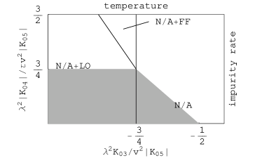
Figure 4: This figure shows the nature of the superconducting state which is realized just below the upper critical line, as well as the type of the transition, for quasi two-dimensional d-wave superconductors, at large paramagnetic, small orbital and impurity effects, and for temperatures close to the tricritical temperature $T^{*}$. (See also the legend of Fig. 2).

From the previous discussion, one can guess that our Ansatz (33) is not the most general. Indeed, in the presence of orbital effect, one should also consider order parameters in the form

$$\Delta=f(z)(A_{n}\varphi_{n}+A_{n+4}\varphi_{n+4}+\ldots),$$

where $n>0$. Therefore, the FFLO phases illustrated in Figs. 3 and 4 may compete with phases corresponding to order parameter with higher Landau level $n>0$. This problem is reserved for further study.

Note that these results are very sensitive to the shape of the Fermi surface. In particular, different topology for the phase diagram would be obtained for anisotropic d-wave superconductor with elliptic Fermi surface.

IV FFLO instability in disordered s-wave superconductor

According to Ref. Asl , instability toward FFLO state formation is always present in s-wave superconductors in the paramagnetic limit. In particular, assuming that the transition from normal to FFLO state is of the second type, such instability occurs at $T^{*}=0.56T_{c}$ in clean systems and at vanishingly small temperature $T_{d}^{*}\simeq-\Delta_{0}/(2\ln\tau\Delta_{0})$ in dirty ones.

On the other hand, a large orbital effect is detrimental to FFLO instability, as shown in clean s-wave superconductors in Ref. Gru . Indeed, it was shown there that the FFLO instability only takes place when the paramagnetic effect, characterized by a Maki parameter $\alpha_{M}^{c}>1.8$, is strong enough.

In this section, we adress the question of FFLO instability in s-wave superconductors with disorder. In particular, we find that the second order transition toward FFLO state exists for any disorder provided that the orbital effect remains small enough. In the dirty limit ($\tau\Delta_{0}\ll 1$), the Maki parameter characterizing its strength must be very large: $\alpha_{M}^{d}>-1/(\tau\Delta_{0}\ln\tau\Delta_{0})$.

As we discussed in the previous sections, transition from normal to conventional superconducting state may change its type. In particular, in dirty systems, such change of the transition type was shown to take place below some critical temperature as soon as $\alpha_{M}^{d}>1$.maki66 Therefore, the FFLO state may either exist as a metastable state below the first order transition line into conventional superconducting state or take place by first order transition with even higher critical field. We do not discuss the question of the type of the transition in the present section.

Let us now derive the result.

At the second order transition in superconducting state, the linearized self-consistency equation (74) is

$$\Delta\ln\frac{T}{T_{c}}+2\pi T\Re\left[\sum_{\nu\geq 0}\left(\frac{1}{\omega_{\nu}}-\frac{\langle{\cal L}_{\nu}\rangle}{1-\frac{1}{2\tau}\langle{\cal L}_{\nu}\rangle}\right)\right]\Delta=0,$$ (47)

where the differential operator $\langle{\cal L}_{\nu}\rangle$ is:

$$\langle{\cal L}_{\nu}\rangle=\int\frac{d\Omega_{\bf{v}}}{4\pi}\frac{1}{\tilde{\Omega}_{\nu}+i\frac{\bf{vD}}{2}}.$$ (48)

The most general form of the solution for the gap at the second order transition is $\Delta=\varphi_{0}(x,y)e^{iqz}$, where $q$ is the FFLO modulation vector and $\varphi_{0}$ is the Abrikosov vortex lattice formed of lowest level Landau functions. Using the identity $1/X=\int_{0}^{\infty}dse^{-sX}$ and the properties of Landau functions, we find that the operator $\langle{\cal L}_{\nu}\rangle$ applied to $\Delta$ yields the eigenvalue:

$$\langle{\cal L}_{\nu}(q)\rangle=\int_{0}^{\infty}ds\exp(-s\tilde{\Omega}_{\nu})\int_{0}^{1}du\qquad\qquad$$ (49)

$$\quad\times\exp\left(-\frac{\pi Hv_{F}^{2}}{8\Phi_{0}}s^{2}(1-u^{2})\right)\cos\left(\frac{suv_{F}q}{2}\right).$$

At $q=0$, Eqs. (47),(49) yield the second order critical line $H_{c2}(T)$ for transition into usual superconducting vortex lattice state. In particular, in the paramagnetic limit the upper critical field is $H_{p}^{(2)}=\Delta_{0}/(2\mu)=H_{p}/\sqrt{2}$ and it does not depend on the disorder. In the clean, orbital limit, the upper critical field is $H_{c20}^{c}=(\gamma e^{2}/2\pi)\Phi_{0}\Delta_{0}^{2}/v_{F}^{2}$. At finite temperature and/or intermediate disorder, $H_{c2}$ must be found numerically.

In the dirty limit, the equations determining the upper critical field simplify greatly. Indeed, integration on $s$ in Eq. (49) is cut off by impurity scattering time, $s\lesssim\tau$. Thus, assuming that $H\ll\Phi_{0}/(v_{F}\tau)^{2}$ (as can be checked consistently later), we may expand the second exponential in Eq. (49) and perform the integration explicitly:

$$\langle{\cal L}_{\nu}(0)\rangle\simeq\left(\frac{1}{\tilde{\Omega}_{\nu}}-\frac{\pi Hv_{F}^{2}}{6\Phi_{0}\tilde{\Omega}_{\nu}^{3}}\right).$$ (50)

Thus, we obtain the implicit equation for $H_{c2}$ in the dirty limit K.Maki :

$$\ln\frac{T}{T_{c}}=\Re\left[\Psi\left(\frac{1}{2}\right)-\Psi\left(\frac{1}{2}+i\frac{\mu H_{c2}}{2\pi T}+\frac{DH_{c2}}{2\Phi_{0}T}\right)\right],$$ (51)

where $D=v_{F}^{2}\tau/3$ is the diffusion constant. In particular, the critical field at zero temperature,

$$H_{c2}(0)=\frac{H_{c20}^{d}}{\sqrt{1+\alpha_{M}^{d2}}},$$ (52)

interpolates between $H_{p}^{(2)}$ in the paramagnetic limit and the upper critical field in the orbital, dirty limit, $H_{c20}^{d}=\Phi_{0}T_{c}/2\gamma D$, with the Maki parameter in the dirty limit defined as: $\alpha_{M}^{d}=\sqrt{2}H_{c20}^{d}/H_{p}=\mu\Phi_{0}/\pi D$.

In general, the critical field defined by Eq. (47) also depends on $q$: $H=H(q)$. The actual critical field corresponds to the maximal value of $H(q)$ with respect to $q$. When it is obtained for $q\neq 0$, second order transition into FFLO state is realized. Along the critical line $H(q=0)$ at given impurity rate and Maki parameter, the triple point below which such transition may occur is defined by $\partial H/\partial(q^{2})|_{q=0}=0$. (One could check that $\partial H/\partial q|_{q=0}=0$ is always true.) In order to obtain $\partial H/\partial(q^{2})|_{q=0}=0$, one can expand Eq. (47) up to the second order in $q$, and obtain:

$$H = H_{c2}(T)+\Lambda q^{2}+{\cal O}(q^{4})$$ (53)

$$\Lambda = \frac{(2\pi T)^{2}}{\mu\Re\left[\zeta\Psi_{1}\left(\frac{1}{2}+\frac{\mu H\zeta}{2\pi T}\right)\right]}\Re\sum_{\nu\geq 0}\left.\frac{\partial\langle{\cal L}_{\nu}(q)\rangle/\partial(q^{2})}{(1-\frac{1}{2\tau}\langle{\cal L}_{\nu}(q)\rangle)^{2}}\right|_{q=0}.$$

where $\zeta=1/\alpha_{M}^{d}+i$. Making use of Eq. (49) and integration by part, one finally obtains the condition $\partial H/\partial(q^{2})|_{q=0}\propto\Lambda=0$ in the form:

$$0=\Re\sum_{\nu\geq 0}\frac{\tilde{\Omega}_{\nu}^{-1}-\langle{\cal L}_{\nu}(0)\rangle}{(1-\frac{1}{2\tau}\langle{\cal L}_{\nu}(0)\rangle)^{2}}.$$ (54)

In particular, at zero temperature this equation defines the minimal Maki parameter which allows existence of FFL0 state. In the dirty limit, Eq. (54) is easily integrated at zero temperature:

$$0 = \Re\int_{0}^{\infty}d\omega\frac{1}{\omega+\frac{1}{2\tau}+i\mu H}\frac{1}{(\omega+\frac{\pi DH}{\Phi_{0}}+i\mu H)^{2}}$$ (55)

$$\simeq \frac{\sqrt{1+(\alpha_{M}^{d})^{2}}}{\alpha_{M}^{d}(\tau\Delta_{0})^{2}}\left(\frac{1}{\alpha_{M}^{d}}-\tau\Delta_{0}\ln\frac{1}{\tau\Delta_{0}}\right)$$

It yields the critical Maki parameter above which FFLO instability exists:

$$\alpha_{M}^{d}\simeq\frac{1}{\tau\Delta_{0}\ln\frac{1}{\tau\Delta_{0}}}.$$ (56)

Therefore, FFLO instability is present in dirty superconductors provided that the orbital effect is small enough.

V Conclusion

In conclusion, we derived microscopically the generalized Ginzburg-Landau free energy functional which is adequate to describe conventional and unconventional singlet superconductors in the presence of paramagnetic, orbital and impurity effects. This free energy was used to predict the superconducting phase diagrams of three-dimensional s-wave superconductors and quasi-two-dimensional d-wave superconductors under magnetic field perpendicular to the conducting layers. These phase diagrams prove to be quite different and to be very sensitive to geometrical effects such as the nature of the order parameter and the shape of the Fermi surface. In particular, we found that impurities tend to favor the transition from normal state to the Abrikosov vortex lattice state, with the change of the transition type as the temperature is lowered in the s-wave case, while they tend to favor the transition from normal state to the FFLO state with vortex lattice plus additional modulation of the order parameter along the field direction in the d-wave case. We also found that the orbital effect acts in the opposite direction. That is, it tends to favor transition from normal to the FFLO state in s-wave case, while it tends to favor the transition from normal state to the vortex lattice state with the change of the transition type in the d-wave case.

In addition, we determined the criterion for instability toward non uniform superconducting state in s-wave superconductors in the dirty limit.

Appendix A Free energy functional in superconductor doped by impurities

The free energy functional expanded over the order parameter for superconducting state with pairing interaction

$$V({\bf k},{\bf k}^{\prime})=-V\psi(\hat{\bf k})\psi(\hat{\bf k}^{\prime})$$ (57)

has the following form

$$F=\sum_{{\bf q}}\frac{|\Delta_{{\bf q}}|^{2}}{V}-$$

$$T\sum_{\omega}\sum_{{\bf k}{\bf k}^{\prime}{\bf q}^{\prime}}G^{\omega}({\bf k},{\bf k}^{\prime})G^{-\omega}(-{\bf k}+{\bf q},-{\bf k}^{\prime}+{\bf q}^{\prime})\Delta^{*}_{{\bf k},{\bf q}}\Delta_{{\bf k}^{\prime},{\bf q}^{\prime}}$$

$$+\frac{T}{2}\sum_{\omega}\sum_{{\bf q}_{1}-{\bf q}_{2}={\bf q}_{4}-{\bf q}_{3}}\sum_{{\bf k}{\bf p}{\bf l}{\bf m}}G^{\omega}({\bf k},{\bf p})\Delta^{*}_{{\bf k},{\bf q}_{1}}$$

$$G^{-\omega}(-{\bf k}+{\bf q}_{1},-{\bf l}+{\bf q}_{1})\Delta_{{\bf l},{\bf q}_{2}}$$

$$G^{\omega}({\bf m}-{\bf q}_{1}+{\bf q}_{2},{\bf l}-{\bf q}_{1}+{\bf q}_{2})\Delta^{*}_{{\bf m},{\bf q}_{3}}$$

$$G^{-\omega}(-{\bf m}+{\bf q}_{4},-{\bf p}+{\bf q}_{4})\Delta_{{\bf p},{\bf q}_{4}}.$$ (58)

Here, the order parameter is given by Fourier transformation of Eqn (1)

$$\Delta_{{\bf k},{\bf q}}=\psi(\hat{\bf k})\Delta_{{\bf q}}=\int d^{3}r\exp(-i{\bf q}{\bf r})\Delta({\bf k},{\bf r}),$$

and $G^{\omega}({\bf k},{\bf p})$ is exact electron Green function in normal metal with arbitrary configuration of impurities. Averaging of the free energy over impurity configurations demands calculation of averages of vertices Gor60

$$A_{{\bf k},{\bf q}}=$$

$$\sum_{{\bf k}^{\prime}{\bf q}^{\prime}}\overline{G^{\omega}({\bf k},{\bf k}^{\prime})G^{-\omega}(-{\bf k}+{\bf q},-{\bf k}^{\prime}+{\bf q}^{\prime})\Delta_{{\bf k}^{\prime},{\bf q}^{\prime}}}$$ (59)

obeying of equation

$$A_{{\bf k},{\bf q}}=\sum_{{\bf k}^{\prime}{\bf q}^{\prime}}\overline{G^{\omega}({\bf k},{\bf k}^{\prime})}~{}\overline{G^{-\omega}(-{\bf k}+{\bf q},-{\bf k}^{\prime}+{\bf q}^{\prime}})$$

$$[\Delta_{{\bf k}^{\prime},{\bf q}^{\prime}}+nu^{2}\sum_{{\bf p}}A_{{\bf p},{\bf q}^{\prime}}],$$ (60)

where $nu^{2}=1/2\pi N_{0}\tau$, $n$ is impurity concentration, $u$ is the amplitude of scattering, and $\tau$ is mean free time of scattering of quasiparticles. Substituting the Green functions by its average

$$\overline{G^{\omega}({\bf k},{\bf p})}=G^{\omega}({\bf k})\delta({\bf k}-{\bf p}),$$ (61)

$$G^{\pm\omega}({\bf k})=\frac{1}{\pm i(\tilde{\omega}_{\nu}-i\mu H)-\xi({\bf k})}$$ (62)

we obtain from (60)

$$A_{{\bf k},{\bf q}}=G^{\omega}({\bf k})G^{-\omega}(-{\bf k}+{\bf q})\bar{\Delta}_{{\bf k},{\bf q}},$$ (63)

where

$$\bar{\Delta}_{{\bf k},{\bf q}}=\Delta_{{\bf k},{\bf q}}+nu^{2}\sum_{{\bf p}}A_{{\bf p},{\bf q}},$$ (64)

and

$$\sum_{{\bf k}}A_{{\bf k},{\bf q}}=\frac{\sum\limits_{{\bf k}}G^{\omega}({\bf k})G^{-\omega}(-{\bf k}+{\bf q})\Delta_{{\bf k},{\bf q}}}{1-nu^{2}\sum\limits_{{\bf k}}G^{\omega}({\bf k})G^{-\omega}(-{\bf k}+{\bf q})}.$$ (65)

Then, following the procedure developed in Gor60 , after the averaging of free energy (58) we obtain

$$F=F_{2}+F_{4}$$ (66)

where

$$F_{2}=\sum_{{\bf q}}\frac{|\Delta_{{\bf q}}|^{2}}{V}-$$

$$T\sum_{\omega}\sum_{{\bf k}{\bf q}}G^{\omega}({\bf k})G^{-\omega}(-{\bf k}+{\bf q})\Delta^{*}_{{\bf k},{\bf q}}\bar{\Delta}_{{\bf k},{\bf q}}$$ (67)

$$F_{4}=\frac{T}{2}\sum_{\omega}\sum_{{\bf q}_{1}-{\bf q}_{2}={\bf q}_{4}-{\bf q}_{3}}\left\{\sum_{{\bf k}}G^{\omega}({\bf k})\bar{\Delta}^{*}_{{\bf k},{\bf q}_{1}}\right.$$

$$\left.G^{-\omega}(-{\bf k}+{\bf q}_{1})\bar{\Delta}_{{\bf k},{\bf q}_{2}}G^{\omega}({\bf k}-{\bf q}_{1}+{\bf q}_{2})\bar{\Delta}^{*}_{{\bf k},{\bf q}_{3}}\right.$$

$$\left.G^{-\omega}(-{\bf k}+{\bf q}_{4})\bar{\Delta}_{{\bf k},{\bf q}_{4}}\right.$$

. $$\left.+nu^{2}\sum_{{\bf k}}G^{\omega}({\bf k})\bar{\Delta}^{*}_{{\bf k},{\bf q}_{1}}\right.$$ (68)

$$\left.G^{-\omega}(-{\bf k}+{\bf q}_{1})\bar{\Delta}_{{\bf k},{\bf q}_{4}}G^{-\omega}(-{\bf k}+{\bf q}_{4})\right.$$

$$\left.\sum_{{\bf k}}G^{-\omega}(-{\bf k}+{\bf q}_{1})\bar{\Delta}_{{\bf k},{\bf q}_{2}}G^{-\omega}(-{\bf k}+{\bf q}_{4})\right.$$

$$\left.\bar{\Delta}^{*}_{{\bf k},{\bf q}_{3}}G^{\omega}({\bf k}-{\bf q}_{1}+{\bf q}_{2})\right.$$

$$\left.+nu^{2}\sum_{{\bf k}}G^{-\omega}(-{\bf k}+{\bf q}_{4})\bar{\Delta}_{{\bf k},{\bf q}_{4}}\right.$$

$$\left.G^{\omega}({\bf k})\bar{\Delta}^{*}_{{\bf k},{\bf q}_{3}}G^{\omega}({\bf k}-{\bf q}_{1}+{\bf q}_{2})\right.$$

$$\left.\sum_{{\bf k}}G^{-\omega}(-{\bf k}+{\bf q}_{1})\bar{\Delta}^{*}_{{\bf k},{\bf q}_{1}}\right.$$

$$\left.G^{\omega}({\bf k})\bar{\Delta}_{{\bf k},{\bf q}_{2}}G^{\omega}({\bf k}-{\bf q}_{1}+{\bf q}_{2})\right\}$$

The further calculations are different for different superconducting states. Expanding the quadratic in respect of the order parameter terms up to forth order in respect of ${\bf q}$ and performing $\xi$ integration we obtain for the case of s-pairing

$$\sum_{{\bf k}}G^{\omega}({\bf k})G^{-\omega}(-{\bf k}+{\bf q})\Delta^{*}_{{\bf k},{\bf q}}\bar{\Delta}_{{\bf k},{\bf q}}$$

$$=\frac{\pi N_{0}}{\Omega_{\nu}}\left\{1-\frac{\langle({\bf q}{\bf v})^{2}\rangle}{4\Omega_{\nu}\tilde{\Omega}_{\nu}}+\frac{\langle({\bf q}{\bf v})^{4}\rangle}{16\Omega_{\nu}\tilde{\Omega}_{\nu}^{3}}\right.$$

$$\left.+\frac{(\langle({\bf q}{\bf v})^{2}\rangle)^{2}}{32\tau\Omega_{\nu}^{2}\tilde{\Omega}_{\nu}^{3}}\right\}|\Delta_{{\bf q}}|^{2}.$$ (69)

Corresponding expression for superconducting order parameter transforming according to non-identity representation even in respect of ${\bf k}$ is

$$\sum_{{\bf k}}G^{\omega}({\bf k})G^{-\omega}(-{\bf k}+{\bf q})\Delta^{*}_{{\bf k},{\bf q}}\bar{\Delta}_{{\bf k},{\bf q}}$$

$$=\frac{\pi N_{0}}{\tilde{\Omega}_{\nu}}\left\{1-\frac{\langle({\bf q}{\bf v})^{2}|\psi(\hat{\bf k})|^{2}\rangle}{4\tilde{\Omega}_{\nu}^{2}}+\frac{\langle({\bf q}{\bf v})^{4}|\psi(\hat{\bf k})|^{2}\rangle}{16\tilde{\Omega}_{\nu}^{4}}\right.$$

$$\left.+\frac{|\langle({\bf q}{\bf v})^{2}\psi(\hat{\bf k})\rangle|^{2}}{32\tau\Omega_{\nu}\tilde{\Omega}_{\nu}^{4}}\right\}|\Delta_{{\bf q}}|^{2}.$$ (70)

Here

$$\Omega_{\nu}=\omega_{\nu}-i\mu H,~{}~{}\tilde{\Omega}_{\nu}=\tilde{\omega}_{\nu}-i\mu H,~{}~{}\tilde{\omega}_{\nu}=\omega_{\nu}+\frac{sign~{}\omega_{\nu}}{2\tau}.$$ (71)

Substituting (69) and (70) in (67) and performing Fourier transformation to the coordinate space (accompanied by substitution ${\bf q}\to{\bf D}=-i\nabla+(2\pi/\Phi_{0}){\bf A}$) we come to the quadratic terms in the Eqns (2) and (7) correspondingly.

In terms of the forth order in respect of the order parameter one should calculate $\bar{\Delta}_{{\bf k},{\bf q}}$ up to the second order in ${\bf q}$. For the s-pairing state it is

$$\bar{\Delta}_{{\bf k},{\bf q}}=\frac{\tilde{\Omega}_{\nu}}{\Omega_{\nu}}\left(1-\frac{\langle({\bf q}{\bf v})^{2}\rangle}{8\tau\Omega_{\nu}\tilde{\Omega}_{\nu}^{2}}\right)\Delta_{{\bf q}}$$ (72)

and for a non-identity representation

$$\bar{\Delta}_{{\bf k},{\bf q}}=\left(\psi(\hat{\bf k})-\frac{\langle({\bf q}{\bf v})^{2}\psi(\hat{\bf k})\rangle}{8\tau\Omega_{\nu}\tilde{\Omega}_{\nu}^{2}}\right)\Delta_{{\bf q}}.$$ (73)

It is easy to check that in the latter case in terms of the forth order in respect of the order parameter and up to the second order in ${\bf q}$ one can put just $\bar{\Delta}_{{\bf k},{\bf q}}=\psi(\hat{\bf k})\Delta_{{\bf q}}$.

Substituting (72) and (73) in (68), expanding the Green functions up to the second order in ${\bf q}$, performing the integration over ${\xi}$ and Fourier transformation to the coordinate space we come to the quartic terms in the Eqns (2) and (7) correspondingly.

Appendix B Free energy functional derived from Eilenberger equations

In this appendix we propose another method to derive the superconducting free energies (2) and (7) which are introduced in Sec. II.

The quasiclassical theory of superconductivity forms a convenient framework to study conventional and unconventional superconductors in the presence of magnetic fields or impurities.kopnin In this theory, the superconducting gap is related to the anomalous function $f_{\nu}(\hat{\bf k},{\bf r})$ through:

$$\Delta({\bf r})=\pi TV\sum_{\nu}\langle\psi(\hat{\bf k})^{*}f_{\nu}(\hat{\bf k},{\bf r})\rangle_{\hat{\bf k}},$$ (74)

where the brackets stand for the averaging over the Fermi surface labelled by $\hat{\bf k}$, $V$ and $\psi(\hat{\bf k})$ define the pairing interaction (57). The anomalous function is determined by the set of Eilenberger equations:

$$\frac{i}{2}{\bf vD}f_{\nu}+(\Omega_{\nu}+\frac{1}{2\tau}\langle g_{\nu}\rangle)f_{\nu}=\left(\psi\Delta+\frac{1}{2\tau}\langle f_{\nu}\rangle\right)g_{\nu},$$ (75)

where

$$g_{\nu}=\text{sign}(\omega_{\nu})\sqrt{1-f_{\nu}f^{\dagger}_{\nu}}\quad\text{and}\quad f^{\dagger}_{\nu}=-f^{*}_{-(\nu+1)}.$$ (76)

The magnetic field ${\bf H}=\text{rot}{\bf A}$ is combined with gradient in ${\bf D}=-i\nabla+(2\pi/\Phi_{0}){\bf A}$, and $\Omega_{\nu}=\omega_{\nu}-i\mu H$ where $\omega_{\nu}$ is a Matsubara frequency.

Near the second order transition from normal to superconducting state, the order parameter $\Delta$ is vanishingly small. Moreover, we assume that the order parameter is slowly varying on the scale of the superconducting coherence length. Then we may expand the selfconsistency equation (74) up to the third order terms in the gap, and the fourth order terms in the gradient expansion.

In the following we proceed separately for the cases of identity and non-identity representation.

B.1 Identity representation

For simplicity, we only consider identity represenation with $\psi=1$.

The set of Eilenberger equations can be expanded perturbatively in the gap. In this expansion, $g_{\nu}$ only contains even terms: $g_{\nu}=g_{\nu}^{(0)}+g_{\nu}^{(2)}+\dots$, while $f_{\nu}$ only contains odd terms: $f_{\nu}=f_{\nu}^{(1)}+f_{\nu}^{(3)}+\dots$.

In the zeroth order in $\Delta$, at $\omega_{\nu}>0$, we find $g_{\nu}^{(0)}=1$.

In the first order in $\Delta$, $f_{\nu}^{(1)}$ is the solution of the linearized differential equation (75):

$$\frac{i}{2}{\bf vD}f_{\nu}^{(1)}+\tilde{\Omega}_{\nu}f_{\nu}^{(1)}=\Delta+\frac{1}{2\tau}\langle f_{\nu}^{(1)}\rangle,$$ (77)

where $\tilde{\Omega}_{\nu}=\Omega_{\nu}+1/2\tau$. Expressing $\langle f_{\nu}^{(1)}\rangle$ in terms of $\Delta$, we get:

$$\langle f_{\nu}^{(1)}\rangle=\frac{\langle{\cal L}_{\nu}\rangle}{1-\frac{1}{2\tau}\langle{\cal L}_{\nu}\rangle}\Delta,$$ (78)

where ${\cal L}_{\nu}=(\tilde{\Omega}_{\nu}+i{\bf vD}/2)^{-1}$. Expanding up to the fourth order terms in the gradient expansion, we find:

$$\langle f_{\nu}^{(1)}\rangle=\frac{\Delta}{\tilde{\omega}_{\nu}}-\frac{\langle({\bf vD})^{2}\rangle\Delta}{4\tilde{\omega}_{\nu}^{2}\tilde{\Omega}_{\nu}}+\frac{\langle({\bf vD})^{4}\rangle\Delta}{16\tilde{\omega}_{\nu}^{2}\tilde{\Omega}_{\nu}^{3}}+\frac{\langle({\bf vD})^{2}\rangle^{2}\Delta}{32\tau\tilde{\omega}_{\nu}^{3}\tilde{\Omega}_{\nu}^{3}},$$ (79)

where $\tilde{\omega}_{\nu}=\omega_{\nu}+1/2\tau$.

In the second order in $\Delta$, we find from Eq. (76): $g_{\nu}^{(2)}=-f_{\nu}^{(1)}f_{\nu}^{\dagger(1)}/2$.

In the third order in $\Delta$, on gets from Eq. (75) that $f_{\nu}^{(3)}$ is the solution of the linear differential equation:

$$\frac{i}{2}{\bf vD}f_{\nu}^{(3)}+\tilde{\Omega}_{\nu}f_{\nu}^{(3)}=\Delta g_{\nu}^{(2)}+\frac{1}{2\tau}\langle f_{\nu}^{(3)}\rangle$$

$$+\frac{1}{2\tau}\left(\langle f_{\nu}^{(1)}\rangle g_{\nu}^{(2)}-\langle g_{\nu}^{(2)}\rangle f_{\nu}^{(1)}\right).$$ (80)

We can now express $\langle f_{\nu}^{(3)}\rangle$ in terms of $\Delta$ and we make an expansion up to terms of the second order in the gradient expansion. We obtain:

$$\langle f_{\nu}^{(3)}\rangle=-\frac{\Delta|\Delta|^{2}}{2\tilde{\omega}_{\nu}^{3}}+\frac{1}{8\tilde{\omega}_{\nu}^{3}\tilde{\Omega}_{\nu}^{2}}\left[\langle({\bf vD})^{2}\rangle\Delta|\Delta|^{2}\right.$$

$$\left.+\langle({\bf vD})(|\Delta|^{2}({\bf vD})\Delta+\Delta^{2}({\bf vD})^{*}\Delta^{*})\rangle\right.$$

$$\left.+\Delta\langle|{\bf vD}\Delta)|^{2}\rangle+|\Delta|^{2}\langle({\bf vD})^{2}\Delta\rangle+\Delta^{2}\langle({\bf vD}^{*})^{2}\Delta^{*}\rangle\right]$$

$$+\frac{1}{16\tau\tilde{\omega}_{\nu}^{4}\tilde{\Omega}_{\nu}^{2}}\left[\langle({\bf vD})^{2}\rangle\Delta|\Delta|^{2}+\langle({\bf vD})\Delta^{2}({\bf vD})^{*}\Delta^{*}\rangle\right.$$

$$\left.+|\Delta|^{2}\langle({\bf vD})^{2}\rangle\Delta+\Delta^{2}\langle({\bf vD}^{*})^{2}\rangle\Delta^{*}\rangle\right].$$

At $\omega_{\nu}$ of arbitrary sign, one should substitute $\tilde{\omega}_{\nu}\rightarrow|\omega_{\nu}|-i\mu H\text{sign}\omega_{\nu}$ and $\tilde{\Omega}_{\nu}\rightarrow|\omega_{\nu}|+1/2\tau-i\mu H\text{sign}\omega_{\nu}$ in Eqs. (79), (B.1).

Inserting now Eqs. (79), (B.1) into (74), we can put the selfconsistency equation for the gap in the form:

$$0=\left(\ln\frac{T}{T_{c0}}+2\pi T\sum_{\omega>0}\frac{1}{\omega}-\pi K_{10}\right)\Delta+\frac{\pi K_{21}}{4}\langle({\bf vD})^{2}\rangle\Delta$$

$$-\frac{\pi K_{23}}{16}\langle({\bf vD})^{4}\rangle\Delta-\frac{\pi K_{33}}{32\tau}\langle({\bf vD})^{2}\rangle^{2}\Delta+\frac{\pi K_{30}}{2}\Delta|\Delta|^{2}$$

$$-\frac{\pi K_{32}}{8}\left[4|\Delta|^{2}\langle({\bf vD})^{2}\rangle\Delta+\Delta^{2}\langle({\bf vD}^{*})^{2}\rangle\Delta^{*}\right.$$

$$\left.+3\Delta^{*}\langle({\bf vD}\Delta)\rangle^{2}-2\Delta|\langle({\bf vD}\Delta)\rangle|^{2}\right]$$

$$-\frac{\pi K_{42}}{16\tau}\left[3|\Delta|^{2}\langle({\bf vD})^{2}\rangle\Delta+\Delta^{2}\langle({\bf vD}^{*})^{2}\rangle\Delta^{*}\right.$$

$$\left.+2\Delta^{*}\langle({\bf vD}\Delta)\rangle^{2}-2\Delta|\langle{\bf vD}\Delta\rangle|^{2}\right],$$

where we used the standard regularization rule:

$$\frac{1}{V}=\ln\frac{T}{T_{c0}}+2\pi T\sum_{\omega>0}\frac{1}{\omega},$$ (83)

and the coefficients $K_{nm}$ are defined in Eq. (5). We can check straightforwardly that Eq. (B.1) corresponds to the saddle point equation for the free energy functional (2):

$$\frac{\delta F}{\delta\Delta^{*}({\bf r})}=0.$$ (84)

B.2 Non-identity representation

One should proceed along the same line to derive the gap equation for non-identity representation (when $\langle\psi\rangle=0$). In particular, one can obtain:

$$\langle\psi^{*}f_{\nu}^{(1)}\rangle=\frac{\Delta}{\tilde{\Omega}_{\nu}}-\frac{\langle|\psi|^{2}({\bf vD})^{2}\rangle\Delta}{4\tilde{\Omega}_{\nu}^{3}}+\frac{\langle|\psi|^{2}({\bf vD})^{4}\rangle\Delta}{16\tilde{\Omega}_{\nu}^{5}}$$

$$+\frac{\langle\psi^{*}({\bf vD})^{2}\rangle\langle\psi({\bf vD})^{2}\rangle\Delta}{32\tau\tilde{\omega}_{\nu}\tilde{\Omega}_{\nu}^{5}}\qquad$$ (85)

and

$$\langle\psi^{*}f_{\nu}^{(3)}\rangle=-\frac{1}{2\tilde{\Omega}_{\nu}^{3}}\left(\langle|\psi|^{4}\rangle-\frac{1}{2\tau\tilde{\Omega}_{\nu}}\right)\Delta|\Delta|^{2}$$

$$+\frac{1}{8\tilde{\Omega}_{\nu}^{5}}\langle|\psi|^{4}\left[({\bf vD})^{2}\Delta|\Delta|^{2}+{\bf vD}\left(|\Delta|^{2}({\bf vD}\Delta)\right.\right.$$

$$\left.\left.+\Delta^{2}({\bf vD}\Delta)^{*}\right)+|\Delta|^{2}({\bf vD})^{2}\Delta\right.$$

$$\left.+\Delta^{2}({\bf vD}^{2}\Delta)^{*}+\Delta|{\bf vD}\Delta|^{2}\right]\rangle$$

$$-\frac{1}{16\tau\tilde{\Omega}_{\nu}^{6}}\langle|\psi|^{2}\left[({\bf vD})|\Delta|^{2}({\bf vD})\Delta+({\bf vD})^{2}|\Delta|^{2}\Delta\right.$$

$$\left.+2|\Delta|^{2}({\bf vD})^{2}\Delta+\Delta^{2}({\bf vD}^{*})^{2}\Delta^{*}+\Delta|{\bf vD}\Delta|^{2}\right]\rangle.$$

Inserting now Eqs. (B.2, B.2) into (74), we can put the selfconsistency equation for the gap in the form:

$$0=\left(\ln\frac{T}{T_{c0}}+2\pi T\sum_{\omega>0}\frac{1}{\omega}-\pi K_{01}\right)\Delta$$

$$+\frac{\pi K_{03}}{4}\langle|\psi|^{2}({\bf vD})^{2}\rangle\Delta-\frac{\pi K_{05}}{16}\langle|\psi|^{4}({\bf vD})^{4}\rangle\Delta$$

$$-\frac{\pi K_{15}}{32\tau}\langle\psi^{*}{\bf vD}\rangle\langle\psi{\bf vD}\rangle\Delta+\frac{\pi}{2}\left(\langle|\psi|^{4}\rangle K_{30}-\frac{K_{04}}{2\tau}\right)\Delta|\Delta|^{2}$$

$$-\frac{\pi K_{05}}{8}\left[4|\Delta|^{2}\langle({\bf vD})^{2}\rangle\Delta+\Delta^{2}\langle({\bf vD}^{*})^{2}\rangle\Delta^{*}\right.$$

$$\left.+3\Delta^{*}\langle({\bf vD}\Delta)\rangle^{2}-2\Delta|\langle({\bf vD}\Delta)\rangle|^{2}\right]$$

$$+\frac{\pi K_{06}}{16\tau}\left[5|\Delta|^{2}\langle({\bf vD})^{2}\rangle\Delta+2\Delta^{2}\langle({\bf vD}^{*})^{2}\rangle\Delta^{*}\right.$$

$$\left.+3\Delta^{*}\langle({\bf vD}\Delta)\rangle^{2}-4\Delta|\langle{\bf vD}\Delta\rangle|^{2}\right].$$

We can check straightforwardly that Eq. (B.2) corresponds to the saddle point equation for the free energy functionnal (7).

Appendix C Lowest Landau level approximation

In this Appendix we shall prove that in the limit of small influence of orbital effect (large Maki parameters) the function given by Eq.  (31) is appropriate variational function for the Abrikosov lattice ground state in tetragonal superconductor under magnetic field directed along c-axis. With this purpose let us consider the Hamiltonian of the form

$$H=H_{0}+H_{4},$$ (88)

where

$$H_{0}=\alpha a^{-}a^{+}+\beta[a^{-}a^{+}a^{-}a_{+}+a^{-}a^{-}a_{+}a^{+}$$

$$+a^{-}a^{+}a^{+}a^{-}+a^{+}a^{-}a^{-}a^{+}$$

$$+a^{+}a^{+}a^{-}a^{-}+a^{+}a^{-}a^{+}a^{-}],$$ (89)

and

$$H_{4}=\gamma(a^{+})^{4}+\delta(a^{-})^{4}.$$ (90)

The dimensionless differential operators $a^{\pm}=\lambda D^{\pm}$ act on the Landau states $\phi_{n}(x,y),~{}~{}n=0,1,2,\ldots$ as follows

$$a^{-}\phi_{n}=\sqrt{n}\phi_{n-1},~{}~{}~{}~{}a^{+}\phi_{n}=\sqrt{n+1}\phi_{n+1},$$ (91)

such that

$$H_{0}\phi_{0}=\varepsilon_{0}\phi_{0},~{}~{}~{}\varepsilon_{0}=\alpha+3\beta,$$ (92)

and

$$H_{0}\phi_{4}=\varepsilon_{4}\phi_{4},~{}~{}~{}\varepsilon_{4}=5\alpha+123\beta.$$ (93)

Let us consider variational wave function

$$\phi=\phi_{0}+a_{4}\phi_{4}$$ (94)

with $a_{4}$ as a variational parameter and calculate the expectation value

$$\frac{\int dxdy\phi H\phi}{\int dxdy|\phi|^{2}}=\frac{\varepsilon_{0}+\sqrt{24}(\gamma+\delta)a_{4}+\varepsilon_{4}a_{4}^{2}}{1+a_{4}^{2}}.$$ (95)

The minimum of this expression is determined as solution of the equation

$$(\gamma+\delta)a_{4}^{2}-\frac{2(\varepsilon_{4}-\varepsilon_{0})}{\sqrt{24}}a_{4}-(\gamma+\delta)=0$$ (96)

It is clear that at $\gamma=\delta=0$ in other words at $H=H_{0}$ the variational parameter $a_{4}=0$. In general

$$a_{4}=\nu-\nu\sqrt{1+1/\nu^{2}}\approx-\frac{1}{2\nu},$$ (97)

where

$$\nu=\frac{\varepsilon_{4}-\varepsilon_{0}}{\sqrt{24}(\gamma+\delta)}.$$ (98)

The values of coefficients we used are

$$\alpha=\frac{\pi N_{0}K_{03}\langle|\psi|^{2}v_{\perp}^{2}\rangle}{8\lambda^{2}},$$ (99)

$$\beta=-\frac{\pi N_{0}K_{05}\langle|\psi|^{2}v_{\perp}^{4}\rangle}{64\lambda^{4}},$$ (100)

and

$$\gamma=\delta=-\frac{\pi N_{0}K_{05}\langle|\psi|^{2}(v_{x}^{4}-6v_{x}^{2}v_{y}^{2}+v_{y}^{4})\rangle}{64\lambda^{4}},$$ (101)

where, for brevity we have written $\alpha,\beta,\gamma$ and $\delta$ in clean limit $\tau\to\infty$). Thus,in the limit of large $\lambda$ we obtain

$$\nu\approx\frac{16K_{03}\lambda^{2}\langle|\psi|^{2}v_{\perp}^{2}\rangle|}{\sqrt{6}(-K_{05})\langle|\psi|^{2}(v_{x}^{4}-6v_{x}^{2}v_{y}^{2}+v_{y}^{4})\rangle|}$$ (102)

Hence, $\nu\propto\lambda^{2}$ and our variational parameter proves to be small as

$$a_{4}=O\left(\frac{\xi_{0}^{2}}{\lambda^{2}}\right)~{}\cong~{}O\left(\frac{1}{\alpha_{M}}\right).$$ (103)

References

- (1) L.P.Gor’kov, Zh. Eksp.Teor.Fiz. 37, 1407 (1959) [Sov. Phys. JETP 37, 998 (1960)].
- (2) N.R.Werthamer, E.Helfand and P.C.Hohenberg, Phys.Rev. 147, 295 (1966).
- (3) A.M.Clogston, Phys.Rev.Lett. 9, 266 (1962).
- (4) B.S.Chandrasekhar, Appl.Phys.Lett. 1, 7 (1962).
- (5) K.Maki, Physics 1, 127 (1964).
- (6) G.Sarma, J. Phys.Chem.Solids 24, 1029 (1963).
- (7) K.Maki and T.Tsuneto, Progr.Theor.Phys. 31, 945 (1964).
- (8) D.Saint-James, G.Sarma, E.J.Thomas, Type II Superconductivity (Pergamon, New York, 1969).
- (9) P.Fulde and R.A.Ferrell, Phys.Rev. 135, A550 (1964).
- (10) A.I.Larkin and Yu.N.Ovchinnikov, Zh. Eksp.Teor.Fiz. 47, 1136 (1964) [Sov. Phys. JETP 20, 762 (1965)].
- (11) J.A.Bowers and K.Rajagopal, Phys.Rev.D 66, 065002 (2002).
- (12) A.I.Buzdin and H.Kachkachi, Phys.Lett. A225, 341 (1997).
- (13) C.Mora and R.Combescot, Phys.Rev.B 71, 214504 (2005).
- (14) L.W.Gruenberg and L.Gunther, Phys.Rev.Lett. 16, 996 (1966)
- (15) L.G.Aslamazov, Zh. Eksp.Teor.Fiz. 55, 1477 (1968) [Sov. Phys. JETP 28, 773 (1969)].
- (16) M.Houzet, A.I.Buzdin, Phys.Rev.B 63, 184521 (2001).
- (17) K. Maki and H. Won, Czech J. Phys. 46, 1035 (1996).
- (18) K.V.Samokhin, Physica C 274, 156 (1997).
- (19) Kun Yang, S.L.Sondhi, Phys.Rev.B 57, 8566 (1998).
- (20) A.V.Vorontsov, J.A.Sauls, M.J.Graf, Phys.Rev.B 72, 184501 (2005).
- (21) R.Movshovich, M.Jaine, J.D.Thompson, C.Petrovich, Z.Fisk, P.G.Pagliuso, and J.L.Sarrao, Phys.Rev.Lett. 86, 5152 (2001).
- (22) K.Izawa, H.Yamaguchi, Yu.Matsuda, H.Shishido, R.Settai, and Y.Onuki, Phys.Rev.Lett. 87, 057002 (2001).
- (23) A.Bianchi, R.Movshovich, N.Oeschler, P.Gegenwart, F.Steglich, J.D.Thompson, P.G.Pagliuso, and J.L.Sarrao, Phys.Rev.Lett. 89, 137002 (2002).
- (24) C. F. Miclea, M. Niclas, D. Parker, K. Maki, J. L. Sarrao, J. D. Thompson, G. Sparn, and F. Steglich, Phys. Rev. Lett. 96, 117001 (2006).
- (25) A.Bianchi, R.Movshovich, C.Capan, P.G.Pagliuso, and J.L.Sarrao, Phys.Rev.Lett. 91, 187004 (2003).
- (26) D. F. Agterberg and K. Yang, J. Phys. Condens. Matter 13, 9259 (2001).
- (27) H. Adachi, R. Ikeda, Phys.Rev.B 68, 184510 (2003); R. Ikeda, H. Adachi, Phys.Rev.B 69, 212506 (2004).
- (28) Yu. N. Ovchinnikov, Zh. Eksp.Teor.Fiz. 115, 726 (1999) [JETP 88, 398 (1999)].
- (29) G. Eilenberger, Z.Phys.214, 195 (1968).
- (30) A. I. Larkin and Yu. N. Ovchinnikov, Zh. Eksp.Teor.Fiz. 55, 2262 (1968) [Sov. Phys. JETP 28, 1200 (1969)].
- (31) L. P. Gor’kov, Zh. Eksp.Teor.Fiz. 37, 1407 (1959) [Sov. Phys. JETP 10, 998 (1960)].
- (32) V. P. Mineev and K. V. Samokhin, ”Introduction to nonconventional superconductivity”, Gordon and Breach Sc. Publ., OPA 1999.
- (33) A. A. Abrikosov, Fundamentals of the theory of metals, (North-Holland New York, NY, 1988).
- (34) A. I. Buzdin and J. P. Brison, Phys. Lett. A 218, 359 (1996).
- (35) M. G. Vavilov and V. P. Mineev, Zh. Eksp.Teor.Fiz. 113, 2174 (1998) [JETP 86, 1191 (1998)].
- (36) K. Maki, Phys. Rev. 148, 362-369 (1966).
- (37) K.Maki, Physics 1, 127 (1964).
- (38) N. Kopnin, Theory of nonequilibrium superconductivity (Clarendon Press, Oxford, 2001).