Non-perturbative many-body approach to the Hubbard model and single-particle pseudogap.

Abstract

A new approach to the single-band Hubbard model is described in the general context of many-body theories. It is based on enforcing conservation laws, the Pauli principle and a number of crucial sum-rules. More specifically, spin and charge susceptibilities are expressed, in a conserving approximation, as a function of two irreducible vertices whose values are found by imposing the local Pauli principle $\left\langle n_{\uparrow}^{2}\right\rangle=\left\langle n_{\uparrow}\right\rangle$ as well as the local-moment sum-rule and consistency with the equations of motion in a local-field approximation. The Mermin-Wagner theorem in two dimensions is automatically satisfied. The effect of collective modes on single-particle properties is then obtained by a paramagnon-like formula that is consistent with the two-particle properties in the sense that the potential energy obtained from $Tr\Sigma G$ is identical to that obtained using the fluctuation-dissipation theorem for susceptibilities. Since there is no Migdal theorem controlling the effect of spin and charge fluctuations on the self-energy, the required vertex corrections are included. It is shown that the theory is in quantitative agreement with Monte Carlo simulations for both single-particle and two-particle properties. The theory predicts a magnetic phase diagram where magnetic order persists away from half-filling but where ferromagnetism is completely suppressed. Both quantum-critical and renormalized-classical behavior can occur in certain parameter ranges. It is shown that in the renormalized classical regime, spin fluctuations lead to precursors of antiferromagnetic bands (shadow bands) and to the destruction of the Fermi-liquid quasiparticles in a wide temperature range above the zero-temperature phase transition. The upper critical dimension for this phenomenon is three. The analogous phenomenon of pairing pseudogap can occur in the attractive model in two dimensions when the pairing fluctuations become critical. Simple analytical expressions for the self-energy are derived in both the magnetic and pairing pseudogap regimes. Other approaches, such as paramagnon, self-consistent fluctuation exchange approximation (FLEX), and pseudo-potential parquet approaches are critically compared. In particular, it is argued that the failure of the FLEX approximation to reproduce the pseudogap and the precursors AFM bands in the weak coupling regime and the Hubbard bands in the strong coupling regime is due to inconsistent treatment of vertex corrections in the expression for the self-energy. Treating the spin fluctuations as if there was a Migdal’s theorem can lead not only to quantitatively wrong results but also to qualitatively wrong predictions, in particular with regard to the the single-particle pseudogap.

I Introduction

Understanding all the consequences of the interplay between band structure effects and electron-electron interactions remains one of the present-day goals of theoretical solid-state Physics. One of the simplest model that contains the essence of this problem is the Hubbard model. In the more than thirty years[1][2] since this model was formulated, much progress has been accomplished. In one dimension,[3][4] various techniques such as diagrammatic resummations,[5] bosonization,[6] renormalization group[7][8] and conformal approaches[9][10] have lead to a very detailed understanding of correlation functions, from weak to strong coupling. Similarly, in infinite dimensions a dynamical mean-field theory[11] leads to an essentially exact solution of the model, although many results must be obtained by numerically solving self-consistent integral equations. Detailed comparisons with experimental results on transition-metal oxides have shown that three-dimensional materials can be well described by the infinite-dimensional self-consistent mean-field approach.[11] Other methods, such as slave-boson[12] or slave-fermion[13] approaches, have also allowed one to gain insights into the Hubbard model through various mean-field theories corrected for fluctuations. In this context however, the mean-field theories are not based on a variational principle. Instead, they are generally based on expansions in the inverse of a degeneracy parameter,[14] such as the number of fermion flavors $N$, where $N$ is taken to be large despite the fact that the physical limit corresponds to a small value of this parameter, say $N=2$. Hence these theories must be used in conjunction with other approaches to estimate their limits of validity.[15] Expansions around solvable limits have also been explored.[16] Finally, numerical solutions,[17] with proper account of finite-size effects, can often provide a way to test the range of validity of approximation methods independently of experiments on materials that are generally described by much more complicated Hamiltonians.

Despite all this progress, we are still lacking reliable theoretical methods that work in arbitrary space dimension. In two dimensions in particular, it is believed that the Hubbard model may hold the key to understanding normal state properties of high-temperature superconductors. But even the simpler goal of understanding the magnetic phase diagram of the Hubbard model in two dimensions is a challenge. Traditional mean-field techniques, or even slave-boson mean-field approaches, for studying magnetic instabilities of interacting electrons fail in two dimensions. The Random Phase Approximation (RPA) for example does not satisfy the Pauli principle, and furthermore it predicts finite temperature antiferromagnetic or spin density wave (SDW) transitions while this is forbidden by the Mermin-Wagner theorem. Even though one can study universal critical behavior using various forms of renormalization group treatments[18][19][20][21][22] or through the self-consistent-renormalized approach of Moriya[23] which all satisfy the Mermin-Wagner theorem in two dimensions, cutoff-dependent scales are left undetermined by these approaches. This means that the range of interactions or fillings for which a given type of ground-state magnetic order may appear is left undetermined.

Amongst the recently developed theoretical methods for understanding both collective and single-particle properties of the Hubbard model, one should note the fluctuation exchange approximation[24] (FLEX) and the pseudo-potential parquet approach.[25] The first one, FLEX, is based on the idea of conserving approximations proposed by Baym and Kadanoff.[26][27] This approach starts with a set of skeleton diagrams for the Luttinger-Ward functional[28] to generate a self-energy that is computed self-consistently. The choice of initial diagrams however is arbitrary and left to physical intuition. In the pseudo-potential parquet approach, one parameterizes response functions in all channels, and then one iterates crossing-symmetric many-body integral equations. While the latter approach partially satisfies the Pauli principle, it violates conservation laws. The opposite is true for FLEX.

In this paper, we present the formal aspects of a new approach that we have recently developed for the Hubbard model [29][30]. The approach is based on enforcing sum rules and conservation laws, rather than on diagrammatic perturbative methods that are not valid for interaction $U$ larger than hopping $t$. We first start from a Luttinger-Ward functional that is parameterized by two irreducible vertices $U_{sp}$ and $U_{ch}$ that are local in space-time. This generates RPA-like equations for spin and charge fluctuations that are conserving. The local-moment sum rule, local charge sum rule, and the constraint imposed by the Pauli principle, $\left\langle n_{\uparrow}^{2}\right\rangle=\left\langle n_{\uparrow}\right\rangle$ then allow us to find the vertices as a function of double occupancy $\left\langle n_{\uparrow}n_{\downarrow}\right\rangle$ (see Eqs.(37) and (38)). Since $\left\langle n_{\uparrow}n_{\downarrow}\right\rangle$ is a local quantity it depends very little on the size of the system and, in principle, it could be obtained reliably using numerical methods, such as for example Monte Carlo simulations. Here, however, we adopt another approach and find $\left\langle n_{\uparrow}n_{\downarrow}\right\rangle$ self-consistently[29] without any input from outside the present theory. This is done by using an ansatz Eq. (40) for the double-occupancy $\left\langle n_{\uparrow}n_{\downarrow}\right\rangle$ that has been inspired by ideas from the local field approach of Singwi et al.[31]. Once we have the spin and charge fluctuations, the next step is to use them to compute a new approximation, Eq.(46), for the single-particle self-energy. This approach to the calculation of the effect of collective modes on single-particle properties[30] is similar in spirit to paramagnon theories.[32] Contrary to these approaches however, we do include vertex corrections in such a way that, if $\Sigma^{\left(1\right)}$ is our new approximation for the self-energy while $G^{\left(0\right)}$ is the initial Green’s function used in the calculation of the collective modes, and $\left\langle n_{\uparrow}n_{\downarrow}\right\rangle$ is the value obtained from spin and charge susceptibilities, then $\frac{1}{2}Tr\left[\Sigma^{\left(1\right)}G^{\left(0\right)}\right]=U\left\langle n_{\uparrow}n_{\downarrow}\right\rangle$ is satisfied exactly. The extent to which $\frac{1}{2}Tr\left[\Sigma^{\left(1\right)}G^{\left(1\right)}\right]$ (computed with $G^{\left(1\right)}$ instead of $G^{\left(0\right)}$) differs from $U\left\langle n_{\uparrow}n_{\downarrow}\right\rangle$ can then be used both as an internal accuracy check and as a way to improve the vertex corrections.

If one is interested only in two-particle properties, namely spin and charge fluctuations, then this approach has the simple physical appeal of RPA but it satisfies key constraints that are always violated by RPA, namely the Mermin-Wagner theorem and the Pauli principle. To contrast it with usual RPA, that has a self-consistency only at the single-particle level, we call it the Two-Particle Self-Consistent approach (TPSC).[29][30][33] The TPSC gives a quantitative description of the Hubbard model not only far from phase transitions, but also upon entering the critical regime. Indeed we have shown quantitative agreement with Monte Carlo simulations of the nearest-neighbor[29] and next-nearest neighbor[34] Hubbard model in two dimensions. Quantitative agreement is also obtained as one enters the narrow critical regime accessible in Monte Carlo simulations. We also have shown[33] in full generality that the TPSC approach gives the $n\rightarrow\infty$ limit of the $O\left(n\right)$ model, while $n=3$ is the physically correct (Heisenberg) limit. In two dimensions, we then recover both quantum-critical[19] and renormalized classical[18] regimes to leading order in $1/n$. Since there is no arbitrariness in cutoff, given a microscopic Hubbard model no parameter is left undetermined. This allows us to go with the same theory from the non-critical to the beginning of the critical regime, thus providing quantitative estimates for the magnetic phase diagram of the Hubbard model, not only in two dimensions but also in higher dimensions[33].

The main limitation of the approach presented in this paper is that it is valid only from weak to intermediate coupling. The strong-coupling case cannot be treated with frequency-independent irreducible vertices, as will become clear later. However, a suitable ansatz for these irreducible vertices in a Luttinger-Ward functional might allow us to apply our general scheme to this limit as well.

Our approach predicts[30] that in two dimensions, Fermi liquid quasiparticles disappear in the renormalized classical regime $\xi_{AFM}\propto\exp(const/T)$, which always precedes the zero-temperature phase transition in two-dimensions. In this regime the antiferromagnetic correlation length becomes larger than the single-particle thermal de Broglie wave length $\xi_{th}(=v_{F}/T),$ leading to the destruction of Fermi liquid quasiparticles with a concomitant appearance of precursors of antiferromagnetic bands (“shadow bands”) with no quasi-particle peak between them. We stress the crucial role of the classical thermal spin fluctuations and low dimensionality for the existence of this effect and contrast our results with the earlier results of Kampf and Schrieffer[35] who used a susceptibility separable in momentum and frequency $\chi_{sp}=f\left({\bf q}\right)g(\omega)$. The latter form of $\chi_{sp}=f\left({\bf q}\right)g(\omega)$ leads to an artifact that dispersive precursors of antiferromagnetic bands can exist at $T=0$ (for details see [36]). We also contrast our results with those obtained in the fluctuation exchange approximation (FLEX), which includes self-consistency in the single particle propagators but neglects the corresponding vertex corrections. The latter approach predicts only the so-called “shadow feature” [36, 37] which is an enhancement in the incoherent background of the spectral function due to antiferromagnetic fluctuations. However, it does not predict[38] the existence of “shadow bands” in the renormalized classical regime. These bands occur when the condition $\omega-\epsilon_{{\bf k}}-\Sigma_{\sigma}({\bf k,}\omega)+\mu=0$ is satisfied. FLEX also predicts no pseudogap in the spectral function $A({\bf k}_{F},\omega)$ at half-filling [38]. By analyzing temperature and size dependence of the Monte Carlo data and comparing them with the theoretical calculations, we argue that the Monte Carlo data supports our conclusion that the precursors of antiferromagnetic bands and the pseudogap do appear in the renormalized classical regime. We believe that the reason for which the FLEX approximation fails to reproduce this effect is essentially the same reason for which it fails to reproduce Hubbard bands in the strong coupling limit. More specifically, the failure is due to an inconsistent treatment of vertex corrections in the self-energy ansatz. Contrary to the electron-phonon case, these vertex corrections have a strong tendency to cancel the effects of using dressed propagators in the expression for the self-energy.

Recently, there have been very exciting developments in photoemission studies of the High-$T_{c}$ materials[39, 40] that show the opening of the pseudogap in single particle spectra above the superconducting phase transition. At present, there is an intense debate about the physical origin of this phenomena and, in particular, whether it is of magnetic or of pairing origin. From the theoretical point of view there are a lot of formal similarities in the description of antiferromagnetism in repulsive models and superconductivity in attractive models. In Sec.(V) we use this formal analogy to obtain a simple analytical expressions for the self-energy in the regime dominated by critical pairing fluctuations. We then point out on the similarities and differences in the spectral function in the case of magnetic and pairing pseudogaps.

Our approach has been described in simple physical terms in Refs.[29] and [30]. The plan of the present paper is as follows. After recalling the model and the notation, we present our theory in Sec.(III). There we point out which exact requirements of many-body theory are satisfied, and which are violated. Before Sec.(III), the reader is urged to read Appendix (A) that contains a summary of sum rules, conservation laws and other exact constraints. Although this discussion contains many original results, it is not in the main text since the more expert reader can refer to the Appendix as need be. We also illustrate in this Appendix how an inconsistent treatment of the self-energy and vertex corrections can lead to the violation of a number of sum rules and inhibit the appearance of the Hubbard bands, a subject also treated in Sec.(VI). Section (IV) compares the results of our approach and of other approaches to Monte Carlo simulations. We study in more details in Sec.(V) the renormalized classical regime at half-filling where, in two dimensions, Fermi liquid quasiparticles are destroyed and replaced by precursors of antiferromagnetic bands well before the $T=0$ phase transition. We also consider in this section the analogous phenomenon of pairing pseudogap which can appear in two dimensions when the pairing fluctuations become critical. The following section Sec.(VI) explains other attempts to obtain precursors of antiferromagnetic bands and points out why approaches such as FLEX fail to see the effect. We conclude in Sec.(VII) with a discussion of the domain of validity of our approach and in Sec.(VIII) with a critical comparison with FLEX and pseudo-potential parquet approaches, listing the weaknesses and strengths of our approach compared with these. A more systematic description and critique of various many-body approaches, as well as proofs of some of our results, appear in appendices.

II Model and definitions

We first present the model and various definitions. The Hubbard model is given by the Hamiltonian,

$$H=-\sum_{<ij>\sigma}t_{i,j}\left(c_{i\sigma}^{\dagger}c_{j\sigma}+c_{j\sigma}^{\dagger}c_{i\sigma}\right)+U\sum_{i}n_{i\uparrow}n_{i\downarrow\,\,\,\,}.$$ (1)

In this expression, the operator $c_{i\sigma}$ destroys an electron of spin $\sigma$ at site $i$. Its adjoint $c_{i\sigma}^{\dagger}$ creates an electron and the number operator is defined by $n_{i\sigma}=$ $c_{i\sigma}^{\dagger}c_{i\sigma}$. The symmetric hopping matrix $t_{i,j}$ determines the band structure, which here can be arbitrary. Double occupation of a site costs an energy $U$ due to the screened Coulomb interaction. We work in units where $k_{B}=1$, $\hbar=1$ and the lattice spacing is also unity, $a=1$. As an example that occurs later, the dispersion relation in the $d$-dimensional nearest-neighbor model is given by

$$\epsilon_{{\bf k}}=-2t\sum_{i=1}^{d}\left(\cos k_{i}\right).$$ (2)

A Single-particle propagators, spectral weight and self-energy.

We will use a “four”-vector notation $k\equiv\left({\bf k,}ik_{n}\right)$ for momentum-frequency space, and $1\equiv\left({\bf r}_{1}{\bf,}\tau_{1}\right)$ for position-imaginary time. For example, the definition of the single-particle Green’s function can be written as

$$G_{\sigma}\left(1{\bf,}2\right)\equiv-\left\langle T_{\tau}c_{1\sigma}\left(\tau_{1}\right)c_{2\sigma}^{\dagger}\left(\tau_{2}\right)\right\rangle\equiv-\left\langle T_{\tau}c_{\sigma}\left(1\right)c_{\sigma}^{\dagger}(2)\right\rangle$$ (3)

where the brackets $\left\langle{}\right\rangle$ represent a thermal average in the grand canonical ensemble, $T_{\tau}$ is the time-ordering operator, and $\tau$ is imaginary time. In zero external field and in the absence of the symmetry breaking $G_{\sigma}\left(1{\bf,}2\right)=G_{\sigma}\left(1{\bf-}2\right)$ and the Fourier-Matsubara transforms of the Green’s function are

$$G_{\sigma}\left(k\right)=\sum_{{\bf r}_{1}}e^{-i{\bf k\cdot r}_{1}}\int_{0}^{\beta}d\tau\ e^{ik_{n}\tau_{1}}G_{\sigma}\left({\bf r}_{1}{\bf,}\tau_{1}\right)\equiv\int d\left(1\right)e^{-ik(1)}G_{\sigma}\left(1\right)$$ (4)

$$G_{\sigma}\left(1\right)=\frac{T}{N}\sum_{k}e^{ik\left(1\right)}G_{\sigma}\left(k\right).$$ (5)

As usual, experimentally observable retarded quantities are obtained from the Matsubara ones by analytical continuation $ik_{n}\rightarrow\omega+i\eta.$ In particular, the single-particle spectral weight $A\left({\bf k,}\omega\right)$ is related to the single-particle propagator by

$$G_{\sigma}\left({\bf k,}ik_{n}\right)=\int\frac{d\omega}{2\pi}\frac{A_{\sigma}\left({\bf k,}\omega\right)}{ik_{n}-\omega}$$ (6)

$$A_{\sigma}\left({\bf k,}\omega\right)=-2\text{Im}G_{\sigma}^{R}\left({\bf k,}\omega\right).$$ (7)

The self-energy obeys Dyson’s equation, leading to

$$G_{\sigma}\left({\bf k,}ik_{n}\right)=\frac{1}{ik_{n}-\left(\epsilon_{{\bf k}}-\mu\right)-\Sigma_{\sigma}\left({\bf k,}ik_{n}\right)}.$$ (8)

It is convenient to use the following notation for real and imaginary parts of the analytically continued retarded self-energy

$$\Sigma_{\sigma}^{R}\left({\bf k,}ik_{n}\rightarrow\omega+i\eta\right)=\Sigma_{\sigma}^{\prime}\left({\bf k,}\omega\right)+i\Sigma_{\sigma}^{\prime\prime}\left({\bf k,}\omega\right).$$ (9)

Causality and positivity of the spectral weight imply that

$$\Sigma_{\sigma}^{\prime\prime}\left({\bf k,}\omega\right)<0.$$ (10)

Finally, let us point out that for nearest-neighbor hopping, the Hamiltonian is particle-hole symmetric at half-filling, $\left(c_{{\bf k}\sigma}\rightarrow c_{{\bf k+Q}\sigma}^{\dagger}\ ;\ c_{{\bf k}\sigma}^{\dagger}\rightarrow c_{{\bf k+Q}\sigma}\right)$ with ${\bf Q=}\left(\pi,\pi\right),$ implying that $\mu=U/2$ and that,

$$G_{\sigma}\left({\bf k},\tau\right)=-G_{\sigma}\left({\bf k+Q},-\tau\right)$$ (11)

$$\left[\Sigma\left({\bf k},ik_{n}\right)-\frac{U}{2}\right]=-\left[\Sigma\left({\bf k+Q},-ik_{n}\right)-\frac{U}{2}\right].$$ (12)

B Spin and charge correlation functions

We shall be primarily concerned with spin and charge fluctuations, which are the most important collective modes in the repulsive Hubbard model. Let the charge and $z$ components of the spin operators at site $i$ be given respectively by

$$\rho_{i}\left(\tau\right)\equiv n_{i\uparrow}\left(\tau\right)+n_{i\downarrow}\left(\tau\right)$$ (13)

$$S_{i}^{z}\equiv n_{i\uparrow}\left(\tau\right)-n_{i\downarrow}\left(\tau\right).$$ (14)

The time evolution here is again that of the Heisenberg representation in imaginary time.

The charge and spin susceptibilities in imaginary time are the responses to perturbations applied in imaginary-time. For example, the linear response of the spin to an external field that couples linearly to the $z$ component

$$e^{-\beta H}\rightarrow e^{-\beta H}T_{\tau}e^{\int d\tau S_{i}^{z}\left(\tau^{\prime}\right)\phi_{i}^{S}\left(\tau^{\prime}\right)}$$ (15)

is given by

$$\chi_{sp}\left({\bf r}_{i}-{\bf r}_{j},\tau_{i}-\tau_{j}\right)=\frac{\delta\left\langle S_{j}\left(\tau_{j}\right)\right\rangle}{\delta\phi_{i}^{S}\left(\tau_{i}\right)}=\left\langle T_{\tau}S_{i}^{z}\left(\tau_{i}\right)S_{j}^{z}\left(\tau_{j}\right)\right\rangle.$$ (16)

In an analogous manner, for charge we have

$$\chi_{ch}\left({\bf r}_{i}-{\bf r}_{j},\tau_{i}-\tau_{j}\right)=\frac{\delta\left\langle\rho_{j}\left(\tau_{j}\right)\right\rangle}{\delta\phi_{i}^{\rho}\left(\tau_{i}\right)}=\left\langle T_{\tau}\rho_{i}\left(\tau_{i}\right)\rho_{j}\left(\tau_{j}\right)\right\rangle-n^{2}.$$ (17)

Here $n\equiv\left\langle\rho_{i}\right\rangle$ is the filling so that the disconnected piece is denoted $n^{2}$. It is well known that when analytically continued, these susceptibilities give physical retarded and advanced response functions. In fact, the above two expressions are the imaginary-time version of the fluctuation-dissipation theorem.

The expansion of the above functions in Matsubara frequencies uses even frequencies. Defining the subscript $ch,sp$ to mean either charge or spin, we have

$$\chi_{ch,sp}\left({\bf q},iq_{n}\right)=\int\frac{d\omega^{\prime}}{\pi}\frac{\chi_{ch,sp}^{\prime\prime}\left({\bf q,}\omega^{\prime}\right)}{\omega^{\prime}-iq_{n}}$$ (18)

$$\chi_{ch}^{\prime\prime}\left({\bf q,}t\right)=\frac{1}{2}\left\langle\left[\rho_{{\bf q}}\left(t\right),\rho_{-{\bf q}}\left(0\right)\right]\right\rangle\quad;\quad\chi_{sp}^{\prime\prime}\left({\bf q,}t\right)=\frac{1}{2}\left\langle\left[S_{{\bf q}}^{z}\left(t\right),S_{-{\bf q}}^{z}\left(0\right)\right]\right\rangle.$$ (19)

The fact that $\chi_{ch,sp}^{\prime\prime}\left({\bf q,}\omega^{\prime}\right)\$is real and odd in frequency in turn means that $\chi_{ch,sp}\left({\bf q},iq_{n}\right)$ is real

$$\chi_{ch,sp}\left({\bf q},iq_{n}\right)=\int\frac{d\omega^{\prime}}{\pi}\frac{\omega^{\prime}\chi_{ch,sp}^{\prime\prime}\left({\bf q,}\omega^{\prime}\right)}{\left(\omega^{\prime}\right)^{2}+\left(q_{n}\right)^{2}}$$ (20)

a convenient feature for numerical calculations. The high-frequency expansion has $1/q_{n}^{2}$ as a leading term so that there is no discontinuity in $\chi_{ch,sp}\left({\bf q},\tau\right)$as $\tau\rightarrow 0,$ contrary to the single-particle case.

III Formal derivation

To understand how to satisfy as well as possible the requirements imposed on many-body theory by exact results, such as those in Appendix (A), it is necessary to start from a general non-perturbative formulation of the many-body problem. We thus first present a general approach to many-body theory that is set in the framework introduced by Martin and Schwinger[42], Luttinger and Ward[28] and Kadanoff and Baym[27][26]. This allows one to see clearly the structure of the general theory expressed in terms of the one-particle irreducible self-energy and of the particle-hole irreducible vertices. These quantities represent projected propagators and there is a great advantage in doing approximations for these quantities rather than directly on propagators.

Our own approximation to the Hubbard model is then described in the subsection that follows the formalism. In our approach, the irreducible quantities are determined from various consistency requirements. The reader who is interested primarily in the results rather than in formal aspects of the theory can skip the next subsection and refer back later as needed.

A General formalism

Following Kadanoff and Baym,[27] we introduce the generating function for the Green’s function

$$\ln Z\left[\phi\right]=\ln\left\langle T_{\tau}e^{-c_{\overline{\sigma}}^{\dagger}\left(\overline{1}\right)c_{\overline{\sigma}}\left(\overline{2}\right)\phi_{\overline{\sigma}}\left(\overline{1},\overline{2}\right)}\right\rangle$$ (21)

where, as above, a bar over a number means summation over position and imaginary time and, similarly, a bar over a spin index means a sum over that spin index. The quantity $Z$ is a functional of $\phi_{\sigma}$, the position and imaginary-time dependent field. $Z$ reduces to the usual partition function when the field $\phi_{\sigma}$ vanishes. The one-particle Green’s function in the presence of this external field is given by

$$G_{\sigma}\left(1,2;\left[\phi\right]\right)=-\frac{\delta\ln Z\left[\phi\right]}{\delta\phi_{\sigma}\left(2,1\right)}$$ (22)

and, as shown by Kadanoff and Baym, the inverse Green’s function is related to the self-energy through

$$G^{-1}=G_{0}^{-1}-\phi-\Sigma.$$ (23)

The self-energy in this expression is a functional of $\phi$.

Performing a Legendre transform on the generating functional $\ln Z\left[\phi\right]$ in Eq.(21) with the help of the last two equations, one can find a functional $\Phi\left[G\right]$ of $G$ that acts as a generating function for the self-energy

$$\Sigma_{\sigma}\left(1,2;\left[G\right]\right)=\frac{\delta\Phi\left[G\right]}{\delta G_{\sigma}\left(2,1\right)}.$$ (24)

The quantity $\Phi\left[G\right]$ is the Luttinger-Ward functional.[28] Formally, it is expressed as the sum of all connected skeleton diagrams, with appropriate counting factors. Conserving approximations start from a subset of all possible connected diagrams for $\Phi\left[G\right]$ to generate both the self-energy and the irreducible vertices entering the integral equation obeyed by response functions. These response functions are then guaranteed to satisfy the conservation laws. They obey integral equations containing as irreducible vertices

$$\Gamma_{\sigma\sigma^{\prime}}^{ir}(1,2;3,4)\equiv\frac{\delta\Sigma_{\sigma}\left(1,2;\left[G\right]\right)}{\delta G_{\sigma^{\prime}}\left(3,4\right)}=\frac{\delta^{2}\Phi\left[G\right]}{\delta G_{\sigma}\left(2,1\right)\delta G_{\sigma^{\prime}}\left(3,4\right)}=\Gamma_{\sigma^{\prime}\sigma}^{ir}(4,3;2,1)$$ (25)

A complete and exact picture of one- and two-particle properties is obtained then as follows. First, the generalized susceptibilities $\chi_{\sigma\sigma^{\prime}}(1,3;2)\equiv-\delta G_{\sigma}\left(1,3\right)/\delta\phi_{\sigma^{\prime}}\left(2^{+},2\right)$ are calculated by taking the functional derivative of $GG^{-1}$ and using the Dyson equation (23) to compute $\delta G^{-1}/\delta\phi$. One obtains[27]

$$\chi_{\sigma\sigma^{\prime}}(1,3;2)=-G_{\sigma}\left(1,2\right)\delta_{\sigma,\sigma^{\prime}}G_{\sigma}\left(2,3\right)+G_{\sigma}\left(1,\overline{2}\right)\Gamma_{\sigma\overline{\sigma}}^{ir}(\overline{2},\overline{3};\overline{4},\overline{5})\chi_{\overline{\sigma}\sigma^{\prime}}(\overline{4},\overline{5};2)G_{\sigma}\left(\overline{3},3\right)$$ (26)

where one recognizes the Bethe-Salpeter equation for the three-point susceptibility in the particle-hole channel. The second equation that we need is automatically satisfied in an exact theory. It relates the self-energy to the response function just discussed through the equation

$$\Sigma_{\sigma}\left(1,2\right)=Un_{-\sigma}\delta\left(1-2\right)+UG_{\sigma}\left(1,\overline{2}\right)\Gamma_{\sigma\sigma^{\prime}}^{ir}(\overline{2},2;\overline{4},\overline{5})\chi_{\sigma^{\prime}-\sigma}(\overline{4},\overline{5};1)$$ (27)

which is proven in Appendix (B).

The diagrammatic representation of these two equations Eqs.(26)(27) appearing in Fig.(1) may make them look more familiar. Despite this diagrammatic representation, we stress that this is only for illustrative purposes. The rest of our discussion will not be diagrammatic.

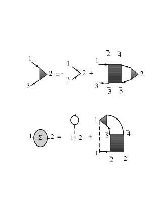
FIG. 1.: The first line is a diagramatic representation of the Bethe-Salpeter equation Eq.(26) for the three point susceptibility and the second line is the corresponding equation Eq.(27) for the self-energy. In the Hubbard model, the Fock contribution is absent, but in general it should be there. Solid lines are Green’s functions and dashed lines represent the contact interaction U. The triangle is the three point vertex, while the three-point susceptibility $\chi(1,3;2)$ is the triangle along with the attached Green’s function. The usual two-point susceptibility is obtained by identifying points $1$ and $3$ in the Bethe-Salpeter equation. The rectangular box is the irreducible four-point vertex in the selected particle-hole channel.

Because of the spin-rotational symmetry the above equations Eqs.(26) and (27) can be decoupled into symmetric (charge) and antisymmetric (spin) parts, by introducing spin and charge irreducible vertices and generalized susceptibilities:

$$\Gamma_{ch}\equiv\Gamma_{\uparrow\downarrow}^{ir}+\Gamma_{\uparrow\uparrow}^{ir}\quad;\quad\Gamma_{sp}\equiv\Gamma_{\uparrow\downarrow}^{ir}-\Gamma_{\uparrow\uparrow}^{ir}$$ (28)

$$\chi_{ch}\equiv 2(\chi_{{}_{\uparrow\downarrow}}+\chi_{{}_{\uparrow\uparrow}})\quad;\quad\chi_{sp}\equiv 2(\chi_{{}_{\uparrow\uparrow}}-\chi_{{}_{\uparrow\downarrow}})$$ (29)

The usual two-point susceptibilities are obtained from the generalized ones as $\chi_{sp,ch}(1,2)=\chi_{sp,ch}(1,1^{+};2)$. The equation Eq.(26) for the generalized spin susceptibility leads to

$$\chi_{sp}(1,3;2)=-2G\left(1,2\right)G\left(2,3\right)-\Gamma_{sp}(\overline{2},\overline{3};\overline{4},\overline{5})G\left(1,\overline{2}\right)G\left(\overline{3},3\right)\chi_{sp}(\overline{4},\overline{5};2)$$ (30)

and similarly for charge, but with the plus sign in front of the second term.

Finally, one can write the exact equation Eq.(27) for the self-energy in terms of the response functions as

$$\Sigma_{\sigma}\left(1,2\right)=Un_{-\sigma}\delta\left(1-2\right)+\frac{U}{4}\left[\Gamma_{sp}(\overline{2},2;\overline{4},\overline{5})\chi_{sp}(\overline{4},\overline{5};1)+\Gamma_{ch}(\overline{2},2;\overline{4},\overline{5})\chi_{ch}(\overline{4},\overline{5};1)\right]G_{\sigma}\left(1,\overline{2}\right).$$ (31)

Our two key equations are thus those for the three-point susceptibilities, Eq.(30), and for the self-energy, Eq.(31). It is clear from the derivation in Appendix (B) that these equations are intimately related.

B Approximations through local irreducible vertices.

1 Conserving approximation for the collective modes.

In formulating approximation methods for the many-body problem, it is preferable to confine our ignorance to high-order correlation functions whose detailed momentum and frequency dependence is not singular and whose influence on the low energy Physics comes only through averages over momentum and frequency. We do this here by parameterizing the Luttinger-Ward functional by two constants $\Gamma_{\uparrow\downarrow}^{ir}$ and $\Gamma_{\uparrow\uparrow}^{ir}$. They play the role of particle-hole irreducible vertices that are eventually determined by enforcing sum rules and a self-consistency requirement at the two-particle level. In the present context, this functional can be also considered as the interacting part of a Landau functional. The ansatz is,

$$\Phi\left[G\right]=\frac{1}{2}G_{\overline{\sigma}}\left(\overline{1},\overline{1}^{+}\right)\Gamma_{\overline{\sigma}\overline{\sigma}}^{ir}G_{\overline{\sigma}}\left(\overline{1},\overline{1}^{+}\right)+\frac{1}{2}G_{\overline{\sigma}}\left(\overline{1},\overline{1}^{+}\right)\Gamma_{\overline{\sigma}-\overline{\sigma}}^{ir}G_{-\overline{\sigma}}\left(\overline{1},\overline{1}^{+}\right).$$ (32)

As in every conserving approximation, the self-energy and irreducible vertices are obtained from functional derivatives as in Eq.(24) and Eq.(25) and then the collective modes are computed from the Bethe-Salpeter equation Eq.(30). The above Luttinger-Ward functional gives a momentum and frequency independent self-energy[43], that can be absorbed in a chemical potential shift. From the Luttinger-Ward functional, one also obtains two local particle-hole irreducible vertices $\Gamma_{\sigma\sigma}^{ir}$ and $\Gamma_{\sigma-\sigma}^{ir}$

$$\Gamma_{\sigma\overline{\sigma}}^{ir}(2,3;4,5)\equiv\frac{\delta\Sigma_{\sigma}\left(2,3\right)}{\delta G_{\sigma^{\prime}}\left(4,5\right)}=\delta\left(2-5\right)\delta\left(3-4\right)\delta\left(4^{+}-5\right)\Gamma_{\sigma\sigma^{\prime}}^{ir}.$$ (33)

We denote the corresponding local spin and charge irreducible vertices as

$$U_{sp}\equiv\Gamma_{\sigma-\sigma}^{ir}-\Gamma_{\sigma\sigma}^{ir}\quad;\quad U_{ch}\equiv\Gamma_{\sigma-\sigma}^{ir}+\Gamma_{\sigma\sigma}^{ir}.$$ (34)

Notice now that there are only two equal-time, equal-point (i.e. local) two-particle correlation functions in this problem, namely $\langle n_{\uparrow}n_{\downarrow}\rangle$ and $\langle n_{\uparrow}^{2}\rangle=\langle n_{\downarrow}^{2}\rangle=\langle n_{\downarrow}\rangle=n/2.$ The last one is completely determined by the Pauli principle and by the known filling factor, while $U\langle n_{\uparrow}n_{\downarrow}\rangle$ is the expectation value of the interaction term in the Hamiltonian. Only one of these two correlators, namely $U\langle n_{\uparrow}n_{\downarrow}\rangle$, is unknown. Assume for the moment that it is known. Then, we can use the two sum rules Eqs.(A18) and (A17) that follow from the fluctuation-dissipation theorem and from the Pauli principle to determine the two trial irreducible vertices from the known value of this one key local correlation functions. In the present notation, these two sum rules are

$$\chi_{ch}\left(1,1^{+}\right)=\frac{T}{N}\sum_{{\bf q}}\sum_{iq_{n}}\chi_{ch}({\bf q,}iq_{n})=\left\langle n_{\uparrow}\right\rangle+\left\langle n_{\downarrow}\right\rangle+2\left\langle n_{\uparrow}n_{\downarrow}\right\rangle-n^{2}$$ (35)

$$\chi_{sp}\left(1,1^{+}\right)=\frac{T}{N}\sum_{{\bf q}}\sum_{iq_{n}}\chi_{sp}({\bf q,}iq_{n})=\left\langle n_{\uparrow}\right\rangle+\left\langle n_{\downarrow}\right\rangle-2\left\langle n_{\uparrow}n_{\downarrow}\right\rangle$$ (36)

and since the spin and charge susceptibilities entering these equations are obtained by solving the Bethe-Salpeter Eq.(30) with the constant irreducible vertices Eqs.(33)(34) we have one equation for each of the irreducible vertices

$$n+2\langle n_{\uparrow}n_{\downarrow}\rangle-n^{2}=\frac{T}{N}\sum_{q}\frac{\chi_{0}(q)}{1+\frac{1}{2}U_{ch}\chi_{0}(q)},$$ (37)

$$n-2\langle n_{\uparrow}n_{\downarrow}\rangle=\frac{T}{N}\sum_{\widetilde{q}}\frac{\chi_{0}(q)}{1-\frac{1}{2}U_{sp}\chi_{0}(q)}.$$ (38)

We used our usual short-hand notation for wave vector and Matsubara frequency $q=({\bf q,}iq_{n})$. Since the self-energy corresponding to our trial Luttinger-Ward functional is constant, the irreducible susceptibilities take their non-interacting value $\chi_{0}(q).$

The local Pauli principle $\langle n_{\downarrow}^{2}\rangle=\langle n_{\downarrow}\rangle$ leads to the following important sum-rule

$$\frac{T}{N}\sum_{{\bf q}}\sum_{iq_{n}}\left[\chi_{sp}\left({\bf q},iq_{n}\right)+\chi_{ch}\left({\bf q},iq_{n}\right)\right]=2n-n^{2},$$ (39)

which can be obtained by adding Eqs.(38),(37). This sum-rule implies that effective interactions for spin $U_{sp}$ and charge $U_{ch}$ channels must be different from one another and hence that ordinary RPA is inconsistent with the Pauli principle (for details see Appendix (A 3)).

Eqs.(37) and (38) determine $U_{sp}$ and $U_{ch}$ as a function of double occupancy $\langle n_{\uparrow}n_{\downarrow}\rangle$. Since double occupancy is a local quantity it depends little on the size of the system. It could be obtained reliably from a number of approaches, such as for example Monte Carlo simulations. However, there is a way to obtain double-occupancy self-consistently[29] without input from outside of the present theory. It suffices to add to the above set of equations the relation

$$U_{sp}=g_{\uparrow\downarrow}(0)\,U\quad;\quad g_{\uparrow\downarrow}(0)\equiv\frac{\langle n_{\uparrow}n_{\downarrow}\rangle}{\langle n_{\downarrow}\rangle\langle n_{\uparrow}\rangle}.$$ (40)

Eqs.(38) and (40) then define a set of self-consistent equations for $U_{sp}$ that involve only two-particle quantities. This ansatz is motivated by a similar approximation suggested by Singwi et al.[31] in the electron gas, which proved to be quite successful in that case. On a lattice we will use it for $n\leq 1$. The case $n>1$ can be mapped on the latter case using particle-hole transformation. In the context of the Hubbard model with on-site repulsion, the physical meaning of Eq. (40) is that the effective interaction in the most singular spin channel, is reduced by the probability of having two electrons with the opposite spins on the same site. Consequently, the ansatz reproduces the Kanamori-Brueckner screening that inhibits ferromagnetism in the weak to intermediate coupling regime (see also below). We want to stress, however, that this ansatz is not a rigorous result like sum rules described above. The plausible derivation of this ansatz can be found in Refs.[31], [29] as well as, in the present notation, in Appendix (C).

We have called this approach Two-Particle Self-Consistent to contrast it with other conserving approximations like Hartree-Fock or Fluctuation Exchange Approximation (FLEX)[24] that are self-consistent at the one-particle level, but not at the two-particle level. This approach[29] to the calculation of spin and charge fluctuations satisfies the Pauli principle $\langle n_{\sigma}^{2}\rangle=\langle n_{\sigma}\rangle=n/2$ by construction, and it also satisfies the Mermin-Wagner theorem in two dimensions.

To demonstrate that this theorem is satisfied, it suffices to show that $\langle n_{\uparrow}n_{\downarrow}\rangle=g_{\uparrow\downarrow}\left(0\right)\langle n_{\uparrow}\rangle\langle n_{\downarrow}\rangle$ does not grow indefinitely. (This guarantees that the constant $\widetilde{C}$ appearing in Eq.(A24) is finite.) To see how this occurs, write the self-consistency condition Eq.(38) in the form

$$n-2\langle n_{\uparrow}n_{\downarrow}\rangle=\frac{T}{N}\sum_{\widetilde{q}}\frac{\chi_{0}(q)}{1-\frac{1}{2}U\frac{\langle n_{\uparrow}n_{\downarrow}\rangle}{\langle n_{\uparrow}\rangle\left\langle n_{\downarrow}\right\rangle}\chi_{0}(q)}.$$ (41)

Consider increasing $\langle n_{\uparrow}n_{\downarrow}\rangle$ on the right-hand side of this equation. This leads to a decrease of the same quantity on the left-hand side. There is thus negative feedback in this equation that will make the self-consistent solution finite. A more direct proof by contradiction has been given in Ref.[29]: suppose that there is a phase transition, in other words suppose that $\langle n_{\uparrow}\rangle\left\langle n_{\downarrow}\right\rangle=\frac{1}{2}U\langle n_{\uparrow}n_{\downarrow}\rangle\chi_{0}(q).$ Then the zero-Matsubara frequency contribution to the right-hand side of Eq.(41) becomes infinite and positive in two dimensions as one can see from phase-space arguments (See Eq.(A24)). This implies that $\langle n_{\uparrow}n_{\downarrow}\rangle$ on the left-hand side must become negative and infinite, but that contradicts the starting hypothesis since $\langle n_{\uparrow}\rangle\left\langle n_{\downarrow}\right\rangle=\frac{1}{2}U\langle n_{\uparrow}n_{\downarrow}\rangle\chi_{0}(q)$ means that $\langle n_{\uparrow}n_{\downarrow}\rangle$ is positive.

Although there is no finite-temperature phase transition, our theory shows that sufficiently close to half-filling (see Sec.(IV C)) there is a crossover temperature $T_{X}$ below which the system enters the so-called renormalized classical regime, where antiferromagnetic correlations grow exponentially. This will be discussed in detail in Sec.(V A 1).

Kanamori-Brueckner screening is also included as we already mentioned above. To see how the screening occurs, consider a case away from half-filling, where one is far from a phase transition. In this case, the denominator in the self-consistency condition can be expanded to linear order in $U$ and one obtains

$$g_{\uparrow\downarrow}\left(0\right)=\frac{\langle n_{\uparrow}n_{\downarrow}\rangle}{\langle n_{\uparrow}\rangle\left\langle n_{\downarrow}\right\rangle}=\frac{1}{1+\Lambda U}$$ (42)

where

$$\Lambda=\frac{2}{n^{2}}\frac{T}{N}\sum_{q}\chi_{0}(q)^{2}.$$ (43)

Clearly, quantum fluctuations contribute to the sum appearing above and hence to the renormalization of $U_{sp}=$ $g_{\uparrow\downarrow}\left(0\right)U.$ The value of $\Lambda$ is found to be near $0.2$ as in explicit numerical calculations of the maximally crossed Kanamori-Brueckner diagrams.[44] At large $U$, the value of $U_{sp}=g_{\uparrow\downarrow}\left(0\right)U\sim 1/\Lambda$ saturates to a value of the order of the inverse bandwidth which corresponds to the energy cost for creating a node in the two-body wave function, in agreement with the Physics described by Kanamori.[2]

To illustrate the dependence of $U_{sp},U_{ch}$ on bare $U$ we give in Fig.(2) a plot of these quantities at half-filling where the correlation effects are strongest. The temperature for this plot is chosen to be above the crossover temperature $T_{X}$ to the renormalized classical regime, in which case the dependence of $U_{sp}$ and $U_{ch}$ on temperature is not significant. As one can see, $U_{sp}$ rapidly saturates to a fraction of the bandwidth, while $U_{ch}$ rapidly increases with $U$, reflecting the tendency to the Mott transition. We have also shown previously in Fig.(2) of Ref.[29] that $U_{sp}$ depends only weakly on filling. Since $U_{sp}$ saturates as a function of $U$ due to Kanamori-Brueckner screening, the crossover temperature $T_{X}$ also saturates as a function of $U$. This is illustrated in Fig.(3) along with the mean-field transition temperature that, by contrast, increases rapidly with $U.$

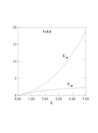
FIG. 2.: Dependence on $U$ of the charge and spin effective interactions (irreducible vertices). The temperature is chosen so that for all $U$, it is above the crossover temperature. In this case, temperature dependence is not significant. The filling is $n=1$

FIG. 3.: Crossover temperature at half-filling as function of $U$ compared with the mean-field transition temperature

Quantitative agreement with Monte Carlo simulations on the nearest-neighbor[29] and next-nearest-neighbor models[34] is obtained[29] for all fillings and temperatures in the weak to intermediate coupling regime $U<8t$. This is discussed further below in Sec.(IV). We have also shown that the above approach reproduces both quantum-critical and renormalized-classical regimes in two dimensions to leading order in the $1/n$ expansion (spherical model)[33].

As judged by comparisons with Monte Carlo simulations[45], the particle-particle channel in the repulsive two-dimensional Hubbard model is relatively well described by more standard perturbative approaches. Although our approach can be extended to this channel as well, we do not consider it directly in this paper. It manifests itself only indirectly through the renormalization of $U_{sp}$ and $U_{ch}$ that it produces.

2 Single-particle properties

As in any implementation of conserving approximations, the initial guess for the self-energy, $\Sigma^{\left(0\right)}$, obtained from the trial Luttinger-Ward functional is inconsistent with the exact self-energy formula Eq.(31). The latter formula takes into account the feedback of the spin and charge collective modes actually calculated from the conserving approximation. In our approach, we use this self-energy formula Eq.(31) in an iterative manner to improve on our initial guess of the self-energy. The resulting formula for an improved self-energy $\Sigma^{\left(1\right)}$ has the simple physical interpretation of paramagnon theories.[46]

As another way of Physically explaining this point of view, consider the following: The bosonic collective modes are weakly dependent on the precise form of the single-particle excitations, as long as they have a quasiparticle structure. In other words, zero-sound or paramagnons exist, whether the Bethe-Salpeter equation is solved with non-interacting particles or with quasiparticles. The details of the single-particle self-energy by contrast can be strongly influenced by scattering from collective modes because these bosonic modes are low-lying excitations. Hence, we first compute the two-particle propagators with Hartree-Fock single-particle Green’s functions, and then we improve on the self-energy by including the effect of collective modes on single-particle properties. The fact that collective modes can be calculated first and self-energy afterwards is reminiscent of renormalization group approaches,[47][8] where collective modes are obtained at one-loop order while the non-trivial self-energy comes out only at two-loop order.

The derivation of the general self-energy formula Eq.(31) given in Appendix (B) shows that it basically comes from the definition of the self-energy and from the equation for the collective modes Eq.(30). This also stands out clearly from the diagrammatic representation in Fig.(1). By construction, these two equations Eqs.(30) and (31) satisfy the consistency requirement $\frac{1}{2}Tr\Sigma G=U\left\langle n_{\uparrow}n_{\downarrow}\right\rangle$ (see Appendix (B)), which in momentum and frequency space can be written as

$$\lim_{\tau\rightarrow 0^{-}}\frac{T}{N}\sum_{k}\Sigma_{\sigma}\left(k\right)G_{\sigma}\left(k\right)e^{-ik_{n}\tau}=U\left\langle n_{\uparrow}n_{\downarrow}\right\rangle,$$ (44)

The importance of the latter sum rule, or consistency requirement, for approximate theories should be clear from the appearance of the correlation function $\langle n_{\uparrow}n_{\downarrow}\rangle$ that played such an important role in determining the irreducible vertices and in obtaining the collective modes. Using the fluctuation dissipation theorem Eqs.(36),(35) this sum-rule can be written in form that explicitly shows the relation between the self-energy and the spin and charge susceptibilities

$$\frac{T}{N}\sum_{k}\left[\Sigma_{\sigma}(k)-Un_{-\sigma}\right]G_{\sigma}(k)=\frac{U}{4}\frac{T}{N}\sum_{q}\left[\chi_{ch}(q)-\chi_{sp}(q)\right].$$ (45)

To keep as much as possible of this consistency, we use on the right-hand side of the self-energy expression Eq.(31) the same irreducible vertices and Green’s functions as those that appear in the collective-mode calculation Eq.(30). Let us call $G^{\left(0\right)}$ the initial Green’s function corresponding to the initial Luttinger-Ward self-energy $\Sigma^{\left(0\right)}.$ Our new approximation for the self-energy $\Sigma^{\left(1\right)}$ then takes the form

$$\Sigma_{\sigma}^{\left(1\right)}\left(k\right)=Un_{-\sigma}+\frac{U}{4}\frac{T}{N}\sum_{q}\left[U_{sp}\chi_{sp}(q)+U_{ch}\chi_{ch}(q)\right]G_{\sigma}^{\left(0\right)}(k+q).$$ (46)

Note that $\Sigma_{\sigma}^{\left(1\right)}\left(k\right)$ satisfies particle-hole symmetry Eq.(12) where appropriate. This self-energy expression (46) is physically appealing since, as expected from general skeleton diagrams, one of the vertices is the bare one $U$, while the other vertex is dressed and given by $U_{sp}$ or $U_{ch}$ depending on the type of fluctuation being exchanged. It is because Migdal’s theorem does not apply for this problem that $U_{sp}$ and $U_{ch}$ are different from the bare $U$ at one of the vertices. $U_{sp}$ and $U_{ch}$ here take care of vertex corrections.[48]

The use of the full $G_{\sigma}(k+q)$ instead of $G_{\sigma}^{0}(k+q)$ in the above expression Eq.(46) would be inconsistent with frequency-independent irreducible vertices. For the collective mode Eq.(30) this is well known to lead to the violation of the conservation laws as was discussed in detail in the previous subsection. Here we insist that the same is true in the calculation of the effect of electronic collective modes on the single-particle properties. Formally, this is suggested by the similarity between the equation for the susceptibility Eq.(30) and that for the self-energy Eq.(31) in terms of irreducible vertices. More importantly, two physical effects would be absent if one were to use full $G$ and frequency independent irreducible vertices. First, upper and lower Hubbard bands would not appear because the $U^{2}/\omega$ high-frequency behavior in Eq.(68) that is necessary to obtain the Hubbard bands would set in too late, as we discuss in Sec.(A 2) and in Sec.(VI A). This result is also apparent from the fact that FLEX calculations in infinite dimension do not find upper and lower Hubbard bands[49] where the exact numerical solution does. The other physical effect that would be absent is precursors of antiferromagnetic bands, Sec.(V) and the pseudogap in $A({\bf k_{F}},\omega)$, that would not appear for reasons discussed in Sec.(VI). We also will see in Sec.(IV) below that FLEX calculations of the single-particle Green’s function, significantly disagree with Monte Carlo data, even away from half-filling, as was already shown in Fig.1 of Ref.[30].

The chemical potential for interacting electrons $\mu$ is found from the usual condition on particle number

$$n=\frac{T}{N}\sum_{k}G_{\sigma}^{\left(1\right)}(k)\exp(-ik_{n}0^{-})=\frac{T}{N}\sum_{k}\frac{\exp(-ik_{n}0^{-})}{i\omega_{n}-\varepsilon_{{\bf k}}+\mu^{(1)}-\Sigma^{(1)}({\bf k},k_{n})}.$$ (47)

This chemical potential $\mu$ is, of course, different from $\mu_{0}$ but the Luttinger sum rule $\sum\theta(-\varepsilon_{{\bf k}}+\mu-\Sigma^{\left(1\right)})=n_{\sigma}$ is satisfied to a high accuracy (about few percent) for all fillings and temperatures $T_{X}\leq T\ll W$. As usual this occurs because the change in $\mu^{(1)}-\mu_{0}$ is compensated by the self-energy shift on the Fermi surface $\Sigma^{(1)}({\bf k}_{F},0)$. For $T<T_{X}$ there is some deviation from the Luttinger sum rule which is due to the appearance of the precursors of the antiferromagnetic bands below $T_{X}$ (Sec. V) which develop into true SDW bands at $T=0$.

It is important to realize that $G^{(0)}$ on the right hand side of the equation for the self-energy $\Sigma$ cannot be calculated as $G^{(0)}=1/(\omega-\varepsilon_{{\bf k}}+\mu^{(1)})$, because otherwise it would not reduce to zero-temperature perturbation theory when it is appropriate. As was pointed out by Luttinger, (see also section A 4) the “non-interacting” Green’s function used in the calculation for $\Sigma$ should be calculated as $G^{(0)}=1/(\omega-\varepsilon_{{\bf k}}-\Sigma^{(n)}({\bf k}_{F},0)+\mu^{(n)})$, where $\mu^{(n)}$ is calculated on the same level of accuracy as $\Sigma^{(n)}({\bf k}_{F},0)$, i.e. from Eq.(47) with $\Sigma^{(n)}({\bf k},ik_{n})$. In our calculation below, we approximate $\mu^{(1)}-\Sigma^{(1)}({\bf k}_{F},0)$ by $\mu_{0}$ because for the coupling strength and temperatures considered in this paper ($U\leq W/2$, $T_{X}\leq T\ll W$) the Luttinger theorem is satisfied to high accuracy and the change of the Fermi surface shape is insignificant. In addition, at half-filling the condition $\mu-\Sigma({\bf k}_{F},0)=\mu_{0}$ is satisfied exactly at any $U$ and $T$ because of particle-hole symmetry. For somewhat larger coupling strengths and away from half-filling, one may try to improve the theory by using $G^{(0)}=1/(\omega-\varepsilon_{{\bf k}}-\Sigma^{(1)}({\bf k}_{F},0)+\mu^{(1)})$, with $\Sigma^{(1)}$ and $\mu$ found self-consistently. However, the domain of validity of our approach is limited to the weak-to-intermediate coupling regime since the strong-coupling regime requires frequency-dependent pseudopotentials (see below).

Finally, let us note that, in the same spirit as Landau theory, the only vertices entering our theory are of the type $\Gamma_{\uparrow\downarrow}$ and $\Gamma_{\uparrow\uparrow},$ or, through Eq.(34), $U_{sp}$ and $U_{ch}$. In other words, we look at the problem from the longitudinal spin and charge particle-hole channel. Consequently, in the contact pseudopotential approximation the exact equation for the self-energy Eq.(31) reduces to our expression Eq. (46) which does not have the factor $3$ in the front of the spin susceptibility. This is different from some paramagnon theories, in which such factor was introduced to take care of rotational invariance. However, we show in Appendix (E 1) that these paramagnon theories are inconsistent with the sum-rule Eq.(45) which relates one and two-particle properties. In our approach, questions about transverse spin fluctuations are answered by invoking rotational invariance $\chi_{sp}^{xx}=\chi_{sp}^{yy}=\chi_{sp}^{zz}$. In particular, one can write the expression for the self-energy Eq.(46) in an explicitly rotationally invariant form by replacing $\chi_{sp}$ by $(1/3)Tr[\chi_{sp}^{\nu\nu}]$. If calculations had been done in the transverse channel, it would have been crucial to do them while simultaneously enforcing the Pauli principle in that channel. In functional integration methods, it is well known that methods that enforce rotational invariance without enforcing the Pauli principle at the same time give unphysical answers, such as the wrong factor $2/3$ in the RPA susceptibility[23] $\chi_{sp}=\chi^{0}/(1-(2/3)U\chi^{0})$ or wrong Hartree-Fock ground state.[50]

3 Internal accuracy check

The quantitative accuracy of the theory will be discussed in detail when we compare with Monte Carlo calculations in the next section. Here we show that we can use the consistency requirement between one- and two-particle properties Eq.(44) to gauge the accuracy of the theory from within the theory itself.

The important advantage of the expression for the self-energy $\Sigma_{\sigma}^{\left(1\right)}\left(k\right)$ given by Eq.(46) is that, as shown in Appendix (B), it satisfies the consistency requirement between one- and two-particle properties Eq.(44), in the following sense

$$\lim_{\tau\rightarrow 0^{-}}\frac{T}{N}\sum_{k}\Sigma_{\sigma}^{\left(1\right)}\left(k\right)G_{\sigma}^{\left(0\right)}\left(k\right)e^{-ik_{n}\tau}=U\left\langle n_{\uparrow}n_{\downarrow}\right\rangle,$$ (48)

Let $G_{\sigma}^{\left(1\right)}$ be defined by $\left[G_{\sigma}^{(1)}\right]^{-1}\equiv G_{0}^{-1}-\Sigma^{\left(1\right)}.$ We can use the fact that in an exact theory we should have $Tr\left[\Sigma_{\sigma}^{\left(1\right)}G_{\sigma}^{\left(1\right)}\right]$ in the above expression instead of $Tr\left[\Sigma_{\sigma}^{\left(1\right)}G_{\sigma}^{\left(0\right)}\right]$ to check the accuracy of the theory. It suffices to compute by how much $Tr\left[\Sigma_{\sigma}^{\left(1\right)}G_{\sigma}^{\left(0\right)}\right]$ differs from $Tr\left[\Sigma_{\sigma}^{\left(1\right)}G_{\sigma}^{\left(1\right)}\right].$ In the parameter range $U<4t$ and $n$,$T$ arbitrary but not too deep in the, soon to be described, renormalized-classical regime, we find that $Tr\left[\Sigma_{\sigma}^{\left(1\right)}G_{\sigma}^{\left(0\right)}\right]$ differs from $Tr\left[\Sigma_{\sigma}^{\left(1\right)}G_{\sigma}^{\left(1\right)}\right]$ by at most $15\%.$ Another way to check the accuracy of our approach is to evaluate the right-hand side of the $f-$sum rule Eqs.(A25) with $n_{{\bf k}\sigma}=G_{\sigma}^{\left(1\right)}\left({\bf k},0^{-}\right)$ and to compare with the result that had been obtained with $f_{{\bf k},\sigma}$. Again we find the same $15\%$ disagreement, at worse, in the same parameter range. As one can expect, this deviation is maximal at half-filling and becomes smaller away from it.

Eq.(46) for the self-energy $\Sigma^{\left(1\right)}$ already gives good agreement with Monte Carlo data but the accuracy can be improved even further by using the general consistency condition Eq.(44) on $Tr\left[\Sigma_{\sigma}^{\left(1\right)}G_{\sigma}^{\left(1\right)}\right]$ to improve on the approximation for vertex corrections. To do so we replace $U_{sp}$ and $U_{ch}$ on the right-hand side of Eq.(46) by $\alpha U_{sp}$ and $\alpha U_{ch}$ with $\alpha$ determined self-consistently in such a way that Eq.(48) is satisfied with $G_{\sigma}^{\left(0\right)}\left(k\right)$ replaced by $G_{\sigma}^{\left(1\right)}\left(k\right)$. For $U<4$, we have $\alpha<1.15$. The slight difference between the irreducible vertices entering the collective modes and the vertex corrections entering the self-energy formula can be understood from the fact that the replacement of irreducible vertices by constants is, in a way, justified by the mean-value theorem for integrals. Since the averages are not taken over the same variables, it is clear that the vertex corrections in the self-energy formula and irreducible vertices in the collective modes do not need to be strictly identical when they are approximated by constants.

Before we move on to comparisons with Monte Carlo simulations, we stress that $\Sigma^{\left(1\right)}$ given by Eq. (46) cannot be substituted back into the calculation of $\chi_{sp,ch}$ by simply replacing $\chi_{0}=G_{0}G_{0}$ with the dressed bubble $\tilde{\chi}_{0}=GG$. Indeed, this would violate conservation of spin and charge and $f$-sum rule. In particular, the condition $\chi_{sp,ch}({\bf q}=0,iq_{n}\neq 0)=0$ that follows from the Ward identity (A31) would be violated as we see in Eq.(A26). In the next order, one is forced to work with frequency-dependent irreducible vertices that offset the unphysical behavior of $\tilde{\chi}_{0}$ at non-zero frequencies.

IV Numerical results and comparisons with Monte Carlo simulations

In this section, we present a few numerical results and comparisons with Monte Carlo simulations. We divide this section in two parts. In the first one we discuss data sufficiently far from half-filling, or at high enough temperature, where size effects are unimportant for systems sizes available in Monte Carlo simulations. In the second part, we discuss data at half-filling. There, size effects become important below the crossover temperature $T_{X}$ where correlations start to grow exponentially (Sec.(V)). All single-particle properties are calculated with our approximation Eq.(46) for the self-energy using the vertex renormalization $\alpha$ explained in the previous section. The results would differ at worse by $15\%$ if we had used $\alpha=1.$

A Far from the crossover temperature $T_{X}$

1 Two-particle properties

We have shown previously in Fig.4a-d of Ref.[29] and in Figs.2-4 and Fig.6 of Ref.[34] that both spin and charge structure factor sufficiently away from the crossover temperature $T_{X}$ are in quantitative agreement with Monte Carlo data for values of $U$ as large as the bandwidth. On the qualitative level, the decrease in charge fluctuations as one approaches half-filling has been explained[29] as a consequence of the Pauli principle embodied in the calculation of the irreducible vertex $U_{ch}.$[51]

Here we present on Fig.(4) and Fig.(5) comparisons with a dynamical quantity, namely the spin susceptibility. Similar comparisons, but with a phenomenological value of $U_{sp}$, have been done by Bulut et al. Ref.[52]. Fig.(4) shows the staggered spin susceptibility as a function of Matsubara frequencies for $n=0.87,$ $T=0.25$ and $U=4$. The effect of interactions is already quite large for the zero-frequency susceptibility. It is enhanced by a factor of over $5$ compared with the non-interacting value. Nevertheless, one can see that the theory and Monte Carlo simulations are in good agreement.

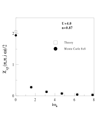
FIG. 4.: Comparisons between Monte Carlo simulations [99] and our theory for the spin susceptibility at $Q=(\pi,\pi)$ as a function of Matsubara frequency. The temperature is $T=0.25$, and the system size $8\times 8$. The factor 1/2 on the vertical axis is due to the fact that the susceptibility in [99] is $\chi_{+-}$ a quantity that is by definition twice smaller then ours and that of [53]

Fig.(5) shows the temperature dependence of the zero-frequency staggered spin susceptibility for the same filling and interaction as in the previous figure. Symbols represent Monte Carlo simulations from Refs.[99] and [53], the solid line is for our theory while dotted and dashed lines are for two versions of FLEX. Surprisingly, the fully conserving FLEX theory, (dashed line) compares worse with Monte Carlo data than the non-conserving version of this theory that neglects the so-called Aslamasov-Larkin diagrams (dotted line). By contrast, our theory is in better agreement with the Monte Carlo data than FLEX for the staggered susceptibility $\chi_{sp}\left({\bf q}=\left(\pi,\pi\right),i\omega_{n}=0\right)$, and at the same time it agrees exactly with the conservation law that states that $\chi_{sp,ch}\left({\bf q}=0,i\omega_{n}\neq 0\right)=0$.

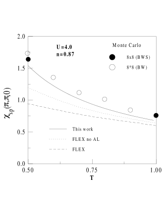
FIG. 5.: Comparisons between the Monte Carlo simulations (BW) and FLEX calculations presented in Fig.19 of Ref. [53] and our theory for the spin susceptibility at $Q=(\pi,\pi)$ as a function of temperature at zero Matsubara frequency. The filled circles (BWS) are from Ref. [99]

Finally, Fig.(6) shows the double occupancy $\left\langle n_{\uparrow}n_{\downarrow}\right\rangle$ as a function of filling for various values of $U$. The symbols again represent Monte Carlo data for $T=1/6$, and the lines are the results of our theory. Everywhere the agreement is very good, except for $n=1,U=4.$ In the latter case, the system is already below the crossover temperature $T_{X}$ to the renormalized classical regime. As explained in Sec.(VII), the appropriate procedure for calculating double occupancy in this case is to take for $\left\langle n_{\uparrow}n_{\downarrow}\right\rangle$ its value (dotted line) at $T_{X}$ instead of using the ansatz Eq.(40). In any case, the difference is not large.

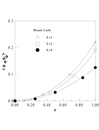
FIG. 6.: Comparisons between the Monte Carlo simulations of Ref.[57] and our theory (solid lines) for the filling dependence of the double occupancy. The results are are for $T=1/6$ as a function of filling and for various values of $U$ except for $U=4$ where the dotted line shows the results of our theory at the crossover temperature $T=T_{X}$.

2 Single-particle properties

Fig.1(a) of Ref.[30] shows $G\left({\bf k,}\tau\right)$ for filling $n=0.875$, temperature $T=0.25$ and $U=4$ for the wave vector on the $8\times 8$ lattice which is closest to the Fermi surface, namely $\left(\pi,0\right)$. Our theory is in agreement with Monte Carlo data and with the parquet approach[53] but in this regime second-order perturbation theory for the self-energy gives the same result. Surprisingly, FLEX is the only theory that disagrees significantly with Monte Carlo data. The good performance of perturbation theory (see also [54]) can be explained in part by compensation between the renormalized vertices and susceptibilities ($U_{sp}<U$, $\chi_{sp}(q)>\chi_{0}(q)$; $U_{ch}>U$, $\chi_{ch}(q)<\chi_{0}(q)$ ).

We have also calculated Re$(\Sigma\left(ik_{n}\right)/ik_{n})$ and compared with the Monte Carlo data in Fig.2a of Ref.[52] obtained at $n=0.87$, $U=4$, $\beta=6.$ Our approach agrees with Monte Carlo data for all frequencies, but again second-order perturbation theory gives similar results.

B Close to crossover temperature $T_{X}$ at half-filling

1 Two-particle properties

The occurrence of the crossover temperature $T_{X}$ at half-filling is perhaps best illustrated in the upper part of Fig.(7) by the behavior of the static structure factor $S_{sp}\left(\pi,\pi\right)$ for $U=4$ as a function of temperature. When the correlation length becomes comparable to the size of the system used in Monte Carlo simulations,[55] the static structure factor starts to increase rapidly, saturating to a value that increases with system size. The solid line is calculated from our theory for an infinite lattice. The Monte Carlo data follow our theoretical curve (solid line) until they saturate to a size-dependent value. The theory correctly describes the static structure factor not only above $T_{X}$ but also as we enter the renormalized classical regime at $T_{X}$. Analytical results for this regime are given in Sec.(V A 1). Note that the RPA mean-field transition temperature for this value of $U$ is more than three times larger than $T_{X}\sim 0.2$. The size-dependence of Monte Carlo data for $S_{sp}\left({\bf q}\right)$ at all other values of ${\bf q\neq}\left(\pi,\pi\right)$ available in simulations is negligible and our calculation for infinite system reproduces this data (not shown).

FIG. 7.: The upper part of the figure, adapted from Ref.[29], shows the temperature dependence of $S_{sp}(\pi,\pi)$ at half-filling $n=1$. The solid line is our theory for an infinite system while symbols are Monte Carlo data from Ref.[56]. The bottom part of the figure, adapted from Ref.[30], shows the behavior of $\tilde{z(T)}=-2G({\bf k}_{F},\beta/2)$ in Eq.(49), as a function of temperature as obtained from Monte Carlo[53] simulations (symbols), from second order pertrubation theory (dashed line) and from our theory for an infinite system (solid line) and for a $16\times 16$ lattice (dashed line).

2 Single-particle properties

Equal-time (frequency integrated) single-particle properties are much less sensitive to precursor effects than dynamical quantities as we now proceed to show. For example, $n\left({\bf k}\right)=G\left({\bf k},0^{-}\right)$ is a sum of $G\left({\bf k},ik_{n}\right)$ over all Matsubara frequencies. We have verified (figure not shown) that $\frac{1}{N}\sum_{{\bf k}\sigma}n_{{\bf k}\sigma}\partial^{2}\epsilon_{{\bf k}}/\partial k_{x}^{2}$ obtained from Monte Carlo simulations[56] is given quite accurately by either second-order perturbation theory or by our theory. This has very important consequences since, for this quantity, the non-interacting value differs from second-order perturbation theory by at most $15\%.$ This means that the numerical value of the right-hand side of the $f$ sum-rule Eq.(A25) is quite close to that obtained from the left-hand side using our expression for the spin and charge susceptibility.

One can also look in more details at $n\left({\bf k}\right)$ itself instead of focusing on a sum rule. Fig.(8) shows a comparison of our theory and of second order perturbation theory with Monte Carlo data for $n\left({\bf k}\right)$ obtained for a set of lattice sizes from $6\times 6$ to $16\times 16$ at $n=1,$ $T=1/6$, $U=4.$ Size effects appear unimportant for this quantity at this temperature. These Monte Carlo data have been used in the past[57] to extract a gap by comparison with mean field SDW theory. Our theory for the same set of lattice sizes is in excellent agreement with Monte Carlo data and predicts a pseudogap at this temperature, as we will discuss below. However, for available values of ${\bf k}$ on finite lattices, second order perturbation theory is also in reasonable agreement with Monte Carlo data for $n\left({\bf k}\right)$. Since second order perturbation theory does not predict a pseudogap, this means that $n\left({\bf k}\right)$ is not really sensitive to the opening of a pseudogap. This is so both because of the finite temperature and because the wave vectors closest to the Fermi surface are actually quite far on the appropriate scale. For this filling, the value of $n\left({\bf k}\right)$ is fixed to $1/2$ on the Fermi surface itself.

FIG. 8.: Occupation number $n(\vec{k})$ as a function of wave vector $\vec{k}$ at half-filling for $T=1/6$, $U=4$, and system sizes $6\times 6$ to $16\times 16$. The symbols are Monte Carlo results from Ref.[57] while the solid line is our theory and the dotted line is the prediction from second order perturbation theory. The dashed line shows the result for $U=0$ as a reference.

It is thus necessary to find a dynamical quantity defined on the Fermi surface whose temperature dependence will allow us to unambiguously identify the pseudogap regime in both theory and in Monte Carlo data. The most dramatic effect is illustrated in the lower part of Fig.(7) where we plot the quantity $\tilde{z}\left(T\right)$ defined by[30][58]

$$\tilde{z}\left(T\right)=-2G\left({\bf k}_{F},\beta/2\right)=\int\frac{d\omega}{2\pi}\frac{A\left({\bf k}_{F},\omega\right)}{\cosh\left(\beta\omega/2\right)}.$$ (49)

The physical meaning of this quantity $\tilde{z}\left(T\right)$ is that it is an average of the single-particle spectral weight $A\left({\bf k}_{F},\omega\right)$ within $T\equiv 1/\beta$ of the Fermi level ($\omega=0$). When quasiparticles exist, this is the best estimate of the usual zero-temperature quasiparticle renormalization factor $z\equiv 1/(1-\partial\Sigma/\partial\omega)$ that can be obtained directly from imaginary-time Monte Carlo data. For non-interacting particles $\tilde{z}\left(T\right)$ is unity. For a normal Fermi liquid it becomes equal to a constant less than unity as the temperature decreases since the width of the quasiparticle peak scales as $T^{2}$ and hence lies within $T$ of the Fermi level. However, contrary to the usual $z\equiv 1/(1-\partial\Sigma/\partial\omega)$ this quantity gives an estimate of the spectral weight $A\left({\bf k}_{F},\omega\right)$ around the Fermi level, even if quasiparticles disappear and a pseudogap forms, as in the present case, (see Sec.(V)).

One can clearly see from the lower part of Fig.(7) that while second-order perturbation theory exhibits typical Fermi-liquid behavior for $\tilde{z}\left(T\right)$, both Monte Carlo data[53] and a numerical evaluation of our expression for the self-energy lead to a rapid fall-off of $\tilde{z}\left(T\right)$ below $T_{X}$ (for $U=4$, $T_{X}\approx 0.2$[29]). The rapid decrease of $\tilde{z}\left(T\right)$ clearly suggests non Fermi-liquid behavior. We checked also that our theory reproduces the Monte Carlo size-dependence. This dependence is explained analytically in Sec.(V A 2). In Ref.[30] we have shown that at half-filling, our theory gives better agreement with Monte Carlo data[53] for $G\left({\bf k}_{F},\tau\right)$ than FLEX, parquet or second order perturbation theory.

To gain a qualitative insight into the meaning of this drop in $\tilde{z}\left(T\right)$, we use the analytical results of the next section to plot in Fig.(9) the value of $A\left({\bf k}_{F},\omega\right).$ This plot is obtained by retaining only the contribution of classical fluctuations Eq.(59) to the self-energy. One sees that above $T_{X}$, there is a quasiparticle but that at $T\sim T_{X}$ a minimum instead of a maximum starts to develop at the Fermi surface $\omega=0.$ Below $T_{X}$, the quasiparticle maximum is replaced by two peaks that are the precursors of antiferromagnetic bands. This is discussed in detail in much of the rest of this paper.

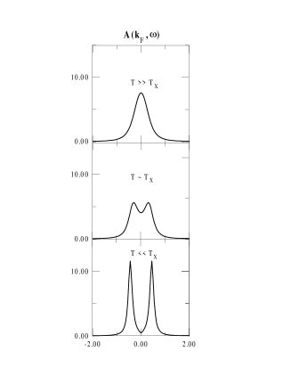
FIG. 9.: Qualitative sketch of the spectral weight at the Fermi wave vector at half-filling for three temperatures. This plot is obtained by retainig only the classical contribution to the self-energy using parameters corresponding to the typical $U=4$ of Monte Carlo simulations. The top plot is for $T>T_{X}$, the middle one for $T\sim T_{X}$ and the bottom one for $T<T_{X}$. The precursors of antiferromagnetic bands would look like this last figure.

C Phase diagram

The main features predicted by our approach for the magnetic phase diagram of the nearest-neighbor hopping model have been given in Ref.[29]. Needless to say, all our considerations apply in the weak to intermediate coupling regime. Note also that both quantum critical and renormalized classical properties of this model have been studied in another publication[33]. The shape of the phase diagram that we find is illustrated in Fig.(10) for $U=2.5$ and $U=4$.

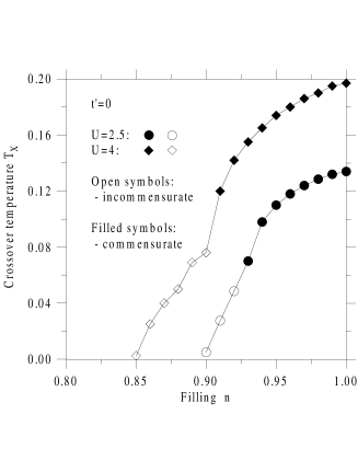
FIG. 10.: Crossover temperature $T_{X}$ as a function of filling for $U=4$ and $U=2.5$. On this crossover line, $\xi^{2}$ is enhanced by a factor of 500 over the bare value. Filled symbols indicate that the crossover is at the antiferromagnetic wave vector, while open symbols indicate a crossover at an incommensurate wave vector. Reproduced with permission from Ref. [100]

At zero temperature and small filling, the system is a paramagnetic Fermi liquid, whatever the value of the interaction $U$ $\left(<W\right)$. Then, as one moves closer to half-filling, one hits a quantum critical point at a value of filling $n_{c}$. Since, $U_{sp}$ in our theory saturates with increasing $U$, the value of $n_{c}$ is necessarily larger than about $n_{c}(U=\infty)=0.68$. At this point, incommensurate order sets in at a wave vector $\left(q_{c},\pi\right)$ or at symmetry-related points. Whatever the value of $U$, the value of $q_{c}$ is contained[29] in the interval $0.74\pi<q_{c}\leq\pi$, increasing monotonously towards $0.74\pi$ as $U$ increases. Since our approach applies only in the paramagnetic phase, at zero temperature we cannot move closer to half-filling. Starting from finite-temperature then, the existence of long-range order at low temperature is signaled by the existence of a crossover temperature $T_{X}\left(n,U\right)$ below which correlations start to grow exponentially. We have already discussed the meaning of $T_{X}\left(n,U\right)$ at half-filling. This crossover temperature becomes smaller and smaller as one moves away from half-filling, until it reaches the quantum-critical point that we just discussed. The correlations that start to grow at $T_{X}\left(n,U\right)$ when $n=1$ are at the antiferromagnetic wave vector, and they stay at this wave vector for a range of fillings $n$. Finally, at some filling, the correlations that start to grow at $T_{X}\left(n,U\right)$ are at an incommensurate value until the quantum-critical point is reached.

Note that the above phase diagram is quite different from the predictions of Hartree-Fock theory mostly because of the strong renormalization of $U_{sp}$. This quantitative change leads to qualitative changes in the Hartree-Fock phase diagram since, for example, Stoner ferromagnetism never occurs in our picture. While the existence of ferromagnetism in the strong coupling limit has been proven only recently[59], the absence of Stoner ferromagnetism in the Hubbard model was already suggested by Kanamori[2] a long time ago and was verified by more recent studies.[44][60][61] More relevant to the present debate though, is the fact that SDW order persists away from half-filling for a finite range of dopings. While this is in agreement with slave-boson approaches[62] and studies[63] using the infinite-dimension methodology,[11] it is in clear disagreement with Monte Carlo simulations[64]. Our approach certainly fails sufficiently below $T_{X}$, but given the successes described above, we believe that it can correctly predict the exponential growth of fluctuations at $T_{X}$. It would be difficult to imagine how one could modify the theory in such a way that the growth of magnetic fluctuations does not occur even at incommensurate wave vectors. Also, such an approach would also need to stop the growth of fluctuations that we find as we approach the quantum critical point along the zero temperature axis, from the low-filling, paramagnetic side, where $T_{X}\left(n<n_{c},U\right)=0$.

It could be that Monte Carlo simulations[64] fail to see long-range order at zero temperature away from half-filling because at zero temperature, in the nearest-neighbor model, this order has a tendency to being incommensurate everywhere except at $n=1$. Furthermore, as we saw above, this incommensuration is in general far from one of the available wave vectors on an $8\times 8$ lattice. It comes close to $\left(0.75\pi,\pi\right)$ only for the largest values of $U$ available by Monte Carlo. Hence, incommensurate order on small lattices is violently frustrated not only by the boundary conditions, but also by the fact that there is no wave vector on what would be the Fermi surface of the infinite system. This means that the electron-electron interaction scatters the electrons at wave-vectors that are not those where the instability would show up, rendering these scatterings not singular. This is clearly an open problem.

V Replacement of Fermi liquid quasiparticles by a pseudogap in two dimensions below $T_{X}.$

One of the most striking consequences of the results discussed in the context of Monte Carlo simulations is the fall of the spectral weight below the temperature $T_{X}$ where antiferromagnetic fluctuations start to grow exponentially in two dimensions. We have already shown in a previous publication[30] that this corresponds to the disappearance of Fermi liquid quasiparticles at the Fermi surface, well above the zero temperature phase transition. We also found that, simultaneously, precursors of the antiferromagnetic bands develop in the single-particle spectrum. Given the simplicity of our approach, it is possible to demonstrate this phenomenon analytically. This is particularly important here because size effects and statistical errors make numerical continuation of the Monte Carlo data to real frequencies particularly difficult. Such analytic continuations using the maximum entropy method[55] have, in the past, lead to a conclusion different from the one obtained later using singular value decomposition[65].

In this section then, we will consider the conditions for which Fermi liquid quasiparticles can be destroyed and replaced by a pseudogap in two dimensions. The major part of this section will be concerned with the single particle pseudogap and the precursors of antiferromagnetic bands in the vicinity of the zero temperature antiferromagnetic phase transition in the positive $U$ Hubbard model. However, it is well known that the problem of superconductivity is formally related to the problem of antiferromagnetism, in particular at half-filling where the nearest-neighbor hopping positive $U$ Hubbard model maps exactly onto the nearest-neighbor negative $U$ Hubbard model. The corresponding canonical transformation maps the ${\bf q=}\left(\pi,\pi\right)$ spin correlations of the repulsive model onto the ${\bf q=0}$ pairing and ${\bf q=}\left(\pi,\pi\right)$ charge correlations of the attractive model while the single-particle Green’s functions of both models are identical. Thus all our results below concerning the opening of the pseudogap in $A\left({\bf k}_{F},\omega\right)$ in the repulsive $U$ half-filled Hubbard model are directly applicable to the attractive $U$ model at half-filling, the only difference being in the physical interpretation. While in the case of repulsive interaction the pseudogap is due to the critical thermal spin fluctuation, in the case of attractive interactions it is, obviously, due to the critical thermal pairing and charge fluctuations. Away from half-filling the mapping between two models is more complicated and the single particle spectra in the pairing pseudogap regime $A\left({\bf k}_{F},\omega\right)$ have important qualitative differences with the single particle spectra in the magnetic pseudogap regime. However, even in this case there are very useful formal similarities between two problems so that in Subsec.(V F) we will give some simple analytical results for the self-energy in the regime dominated by critical pairing fluctuations.

The problem of precursor effects in the repulsive Hubbard model has been first studied by Kampf and Schrieffer[35]. Their analysis however was done at zero temperature and although the precursor effect that they found, called “shadow bands”, looks similar to what we find, there are a number of important differences. For example, they find a quasiparticle between the precursors of antiferromagnetic bands, while we do not. Also, one does not obtain precursors at zero temperature when one uses our more standard expression for the dynamical susceptibility instead of the phenomenological form $\chi_{KShr}=f({\bf q})g(\omega)$ that they use. The physical reason why a function that is separable in both momentum and frequency, such as $\chi_{KShr}$, leads to qualitatively different results than the conventional one has been explained in Ref.[36]. The microscopic justification for $\chi_{KShr}$ is unclear. We comment below on this problem as well as on some of the large related literature that has appeared lately.

Repeating some of the arguments of Ref.[30], we first show by general phase space arguments that the feedback of antiferromagnetic fluctuations on quasiparticles has the potential of being strong enough to destroy the Fermi liquid only in low enough dimension, the upper critical dimension being three. Then we go into more detailed analysis to give explicit analytic expressions for the quasi-singular part of the self-energy, first in Matsubara frequency. The analysis of the self-energy expression directly in real-frequencies is in Appendix (D). The latter analysis is useful to exhibit in the same formalism both the Fermi liquid limit and the non-Fermi liquid limit.

For simplicity we give asymptotics for $n=1$ at the Fermi wave vector, where $\varepsilon({\bf k}_{F}{\bf)}=0$, but similar results apply for $n\neq 1$ as long as there is long-range order at $T=0$ and one is below $T_{X}$. This case is also discussed briefly, but for more details the reader is referred to Ref.[36].

A Upper critical dimension for the destruction of quasiparticles by critical fluctuations.

Before describing the effect of spin fluctuations on quasiparticles, we first describe the so-called renormalized classical regime of spin fluctuations that precedes the zero-temperature phase transition in two dimensions.

1 Renormalized classical regime of spin fluctuations.

The spin susceptibility $\chi_{sp}\left({\bf q},0\right)$ below $T_{X}$ is almost singular at the antiferromagnetic wave vector ${\bf Q}_{2}=\left(\pi,\pi\right)$ because the energy scale $\delta U\equiv U_{mf,c}-U_{sp}$ ($U_{mf,c}\equiv 2/\chi_{0}\left({\bf Q},0\right)$) associated with the proximity to the SDW instability becomes exponentially small.[29] This small energy scale, $\delta U<<T$, leads to the so-called renormalized classical regime for the fluctuations.[66] In this regime, the main contribution to the sum over Matsubara frequencies entering the local-moment sum rule Eq.(38) comes from $iq_{n}=0$ and wave vectors $({\bf q-Q)}^{2}\leq\xi^{-2}$ near ${\bf Q}$. Approximating $\chi_{sp}\left({\bf q},0\right)$ by its asymptotic form

$$\chi_{sp}\left({\bf q},0\right)\approx\frac{1}{U_{sp}\xi_{0}^{2}}\frac{2}{(({\bf q-Q}_{d}{\bf)}^{2}+\xi^{-2})}$$ (50)

where ${\bf Q}_{2}=\left(\pi,\pi\right)$, ${\bf Q}_{3}=\left(\pi,\pi,\pi\right)$ and

$$\xi_{0}^{2}\equiv\frac{-1}{2\chi_{0}\left(Q\right)}\left.\frac{\partial^{2}\chi_{0}\left({\bf q}\right)}{\partial q_{x}^{2}}\right|_{{\bf q=Q}_{d}}\quad;\quad\xi\equiv\xi_{0}(U_{sp}/\delta U)^{1/2}$$ (51)

we obtain, in $d$ dimensions

$$\tilde{\sigma}^{2}=\frac{2T}{U_{sp}\xi_{0}^{2}}\int\frac{d^{d}q}{(2\pi)^{d}}\frac{1}{q^{2}+\xi^{-2}}$$ (52)

where $\tilde{\sigma}^{2}\equiv n-2\langle n_{\uparrow}n_{\downarrow}\rangle-C<1$ is the left-hand side of Eq.(38) minus corrections $C$ that come from the sum over non-zero Matsubara frequencies (quantum effects) and from $({\bf q-Q)}^{2}\gg\xi^{-2}$. There is an upper cutoff to the integral which is less than or of the order of the Brillouin zone size. The important point is that the left-hand side of the above equation Eq.(52) is bounded and weakly dependent on temperature. This implies, as discussed in detail in Ref.[33], that the above equation leads to critical exponents for the correlation length that are in the spherical model ($n\rightarrow\infty)$ universality class. For our purposes, it suffices to notice that the integral converges even when $\xi\rightarrow\infty$ in more than two dimensions. This leads to a finite transition temperature. In two dimensions, the transition temperature is pushed down to zero temperature and, doing the integral, one is left with a correlation length $\xi$ that grows exponentially below $T_{X}$

$$\xi\sim\exp\left(\pi\tilde{\sigma}^{2}\xi_{0}^{2}\frac{U_{sp}}{T}\right).$$ (53)

The important consequence of this is that, below $T_{X}$, the correlation length quickly becomes larger than the single-particle thermal de Broglie wave length $\xi_{th}=v_{F}/\left(\pi T\right)$. This has dramatic consequences on quasiparticles in two dimensions.

2 Effect of critical spin fluctuations on quasiparticles.

When the classical fluctuations ($iq_{n}=0$) become critical, they also give, in two dimensions, a dominant contribution to the self-energy at low frequency. To illustrate what we mean by the classical frequency contribution, neglect the contribution of charge fluctuations and single out the zero Matsubara frequency component from Eq.(46) to obtain

$\displaystyle\Sigma\left({\bf k},ik_{n}\right)\approx Un_{-\sigma}+\frac{U}{4}\frac{T}{N}\sum_{{\bf q}}U_{sp}\chi_{sp}\left({\bf q},0\right)\frac{1}{ik_{n}-\tilde{\epsilon}_{{\bf k+q}}}$

$$+\frac{U}{4}\frac{T}{N}\sum_{{\bf q}}\sum_{iq_{n}\neq 0}U_{sp}\chi_{sp}\left({\bf q},iq_{n}\right)\frac{1}{ik_{n}+iq_{n}-\tilde{\epsilon}_{{\bf k+q}}}$$ (54)

Here, $\tilde{\epsilon}_{{\bf k}}$ is measured relative to the chemical potential. The last term is the contribution from quantum fluctuations. In this last term, the sum over Matsubara frequencies $iq_{n}$ must be done before the analytical continuation of $ik_{n}$ to real frequencies otherwise this analytical continuation would involve going through complex plane poles of the other terms entering the full sum over $iq_{n}.$ The contribution from classical fluctuations, $iq_{n}=0,$ does not have this problem and furthermore it has the correct asymptotic behavior at $ik_{n}\rightarrow\infty$. Hence the contribution of classical fluctuations to the retarded self-energy $\Sigma^{R}\left({\bf k},\omega\right)$ can obtained from the $iq_{n}=0$ term by trivial analytical continuation $ik_{n}\rightarrow\omega+i0.$ Note also that the chemical potential entering $G^{\left(0\right)}$ in the self-energy formula is $\mu_{0}=\mu=0$ at half-filling.

Doing the same substitution as above for the asymptotic form of the spin susceptibility Eq.(50) in the equation for the self-energy Eq.(46) one obtains the following contribution to $\Sigma$ from classical fluctuations

$$\Sigma_{cl}\left({\bf k},ik_{n}\right)\cong\frac{UT}{2\xi_{0}^{2}}\int\frac{d^{d}q}{(2\pi)^{d}}\frac{1}{q^{2}+\xi^{-2}}\frac{1}{ik_{n}-\tilde{\epsilon}_{{\bf k+Q}}-{\bf q\cdot v}_{{\bf k+Q}}}.$$ (55)

where we have expanded $\tilde{\epsilon}_{{\bf k+Q+q}}\simeq\tilde{\epsilon}_{{\bf k+Q}}+{\bf q\cdot v}_{{\bf k+Q}}$. In the case that we consider, namely half-filling and ${\bf k=k}_{F}$, we have $\mu_{0}=\mu=0$ and $\tilde{\epsilon}_{{\bf k}_{F}{\bf+Q}}=0.$ The key point is again that in two dimensions the integral in this equation Eq.(55) is divergent at small $q$ for $\xi=\infty$. In a Fermi liquid, the imaginary part of the self-energy at the Fermi surface $\left(\omega=0\right)$ behaves as $\Sigma_{R}^{\prime\prime}({\bf k}_{F},0)\sim T^{2}$. Here instead, we find a singular contribution

$$\Sigma_{R}^{\prime\prime}({\bf k}_{F},0)\propto T\int d^{d-1}q_{\perp}\frac{1}{q_{\perp}^{2}+\xi^{-2}}\propto T\xi^{3-d}$$ (56)

that is proportional to $\xi$ in $d=2$ and hence is very large $\Sigma_{R}^{\prime\prime}({\bf k}_{F},0)\approx-U\xi/(\xi_{th}\xi_{0}^{2})>1$ when the condition $\xi>\xi_{th}$ is realized. By contrast, 0for $d=3$, $\Sigma_{R}^{\prime\prime}({\bf k}_{F},0)\sim-U\left(\ln\xi\right)/\left(\xi_{0}^{2}\xi_{th}\right)$, so that the Fermi liquid is destroyed only in a very narrow temperature range close the Néel temperature $T_{N}$. Dimensional analysis again suffices to show that in four dimensions the classical critical fluctuations do not lead to any singular behavior. Three dimensions then is the upper critical dimension. As usual, logarithmic corrections exist at the upper critical dimension. The effect will be very small in three dimensions not only because it is logarithmic, but also because the fluctuation regime is very small, extending only in a narrow temperature range around the Néel temperature. By contrast, in two dimensions the effect extends all the way from the crossover temperature, $T_{X}$, which is of the order of the mean-field transition temperature, to zero temperature where the transition is.

Wave vectors near Van Hove singularities are even more sensitive to classical thermal fluctuations. Indeed, near this point the expansion should be of the type $\epsilon_{{\bf k}_{VH}{\bf+q+}\left(\pi,\pi\right)}\propto q_{x}^{2}-q_{y}^{2}$. This leads, in two dimensions, to even stronger divergence in $\Sigma_{R}^{\prime\prime}({\bf k}_{F},0)\propto$ $T\xi^{2}\int dq_{y}\left[\left(2q_{y}^{2}+1\right)\left|q_{y}\right|\right]^{-1}$[36]. Even if the logarithmic divergence is cutoff the prefactor is larger by a factor of $\xi$ compared with points far from the Van Hove singularities.

B Precursors of antiferromagnetic bands in two dimensions.

Let us analyze in more details the consequences of this singular contribution of critical fluctuations to the self-energy in two dimensions. The integral appearing in the two-dimensional version of the expression for the self-energy, Eq.(55), can be performed exactly[67]

$$\Sigma\left({\bf k}_{F},ik_{n}\right)=\frac{U}{2}-i\frac{UT}{8\pi\xi_{0}^{2}\sqrt{k_{n}^{2}-v_{F}^{2}\xi^{-2}}}\ln\frac{k_{n}+\sqrt{k_{n}^{2}-v_{F}^{2}\xi^{-2}}}{k_{n}-\sqrt{k_{n}^{2}-v_{F}^{2}\xi^{-2}}}+{\cal R}.$$ (57)

Here ${\cal R}$ is a regular part.

As a first application, we can use this expression to understand qualitatively both the temperature and size dependence of the Monte Carlo data for $\tilde{z}(T)\$appearing in Fig.(2) of Ref.[30] or in the lower panel of Fig.(7) . Indeed, $\tilde{z}(T)\$can be written as the alternating series $-2G\left({\bf k}_{F},\beta/2\right)=-4T\sum_{n=1}^{\infty}\left(-1\right)^{n}/\left(k_{n}-\Sigma^{\prime\prime}\left({\bf k}_{F},ik_{n}\right)\right)$. Even though the series converges slowly, in the beginning of the renormalized classical regime and for qualitative purposes it suffices to use the first term of this series. Then, using the expressions for the correlation length Eqs. (53) and for the self-energy (57). One finds,

$$\tilde{z}(T)\sim\frac{T^{2}}{\tilde{\sigma}^{2}UU_{sp}}\sqrt{1-\frac{\xi_{th}^{2}}{\xi^{2}}}\quad,\quad T_{X}-T\ll T_{X}.$$ (58)

On the infinite lattice, $\xi$ starts growing exponentially below $T_{X}$, quickly becoming much larger than $\xi_{th}$. This implies $\tilde{z}(T)\simeq T^{2}$. On finite lattices $\xi\sim\sqrt{N}$, which explains the size effect observed in Monte Carlo i.e. smaller $\tilde{z}$ for smaller size $N$, ($\xi_{th}(T_{X})\sim 5$ for Fig.(7)).

The analytic continuation of $\Sigma\left({\bf k}_{F},ik_{n}\right)$ in Eq.(57) is

$$\Sigma^{R}\left({\bf k}_{F},\omega\right)=\frac{U}{2}+\frac{UT}{8\pi\xi_{0}^{2}\sqrt{\omega^{2}+v_{F}^{2}\xi^{-2}}}\left[\ln\left|\frac{\omega+\sqrt{\omega^{2}+v_{F}^{2}\xi^{-2}}}{\omega-\sqrt{\omega^{2}+v_{F}^{2}\xi^{-2}}}\right|-i\pi\right]+{\cal R}.$$ (59)

For the wave vectors ${\bf k}$ away from the Fermi surface the anomalous contribution due to the classical fluctuation has a similar form but with $\omega$ replaced by $(\omega-\tilde{\epsilon}_{{\bf k+Q}})$. When $T>T_{X}$, the correlation length $\xi$ becomes of order unity and, as we will show in Appendix (D), the regular part ${\cal R}$ dominates so that one recovers standard Fermi liquid behavior. Furthermore, even for large correlation length the regular part cannot be neglected when $\omega\gg T$ since the term exhibited here becomes small. Hence we concentrate on small frequencies and on $T<T_{X}$ where the regular part ${\cal R}$ can be neglected.

Exactly at the Fermi level $\left(\omega=0\right)$ we recover the result of the previous section, namely that the imaginary part of the self-energy for $\xi>\xi_{th}$ increases exponentially when the temperature decreases, $\Sigma^{\prime\prime}({\bf k}_{F},0)\sim U\xi/(\xi_{th}\xi_{0}^{2})\propto T\xi\propto T\exp\left(\pi\tilde{\sigma}^{2}\xi_{0}^{2}U_{sp}/T\right)$. The above analysis shows by contradiction that in the paramagnetic state below $T_{X}$ there is no Fermi-liquid quasiparticle at $k_{F},$ yet the symmetry of the system remains unbroken at any finite $T$. Indeed, starting from quasiparticles $\left(G_{\sigma}^{\left(0\right)}\right)$ we found that as temperature decreases, $\Sigma_{R}^{\prime\prime}({\bf k}_{F},0)$ increases indefinitely instead of decreasing, in direct contradiction with the starting hypothesis. By contrast, a self-consistent treatment where we use in Eq.(46) the full $G_{\sigma}$ with a large $\Sigma_{R}^{\prime\prime}({\bf k}_{F},0)$ shows that, for $T<T_{X}$ , $\Sigma_{R}^{\prime\prime}({\bf k}_{F},0)$ remains large in $d=2$ and does not vanish as $T\rightarrow 0$, again confirming that the system is not a Fermi liquid in this regime (See however Sec.(VI B) below). Strong modifications to the usual Fermi liquid picture also persist away from half-filling as long as $T_{X}(n)>0$, as we discuss later.

One can check that the large $\Sigma_{R}^{\prime\prime}({\bf k}_{F},0)$ in two dimensions (for $T<T_{X})$ leads to a pseudogap in the infinite lattice, contrary to the conclusion reached in Ref.[55]. Indeed, instead of a quasiparticle peak, the spectral weight $A\left({\bf k}_{F},\omega\right)\equiv-2$Im$G_{R}\left({\bf k}_{F},\omega\right)$ has a minimum at the Fermi level $\omega=0$ and two symmetrically located maxima away from it. More specifically, for $v_{F}/\xi<\left|\omega\right|<T$ we have

$$A\left({\bf k}_{F},\omega\right)\cong\frac{2\left|\omega\right|UT/(8\xi_{0}^{2})}{[\omega^{2}-UU_{sp}\tilde{\sigma}^{2}/4]^{2}+[UT/(8\xi_{0}^{2})]^{2}}.$$ (60)

The maxima are located at $\omega=\pm\sqrt{UU_{sp}}\tilde{\sigma}/2$. These two maxima away from zero frequency correspond to precursors of the zero-temperature antiferromagnetic (or SDW) bands (shadow bands[35]).There is no quasiparticle peak between these two maxima when $\xi>\xi_{th}$. This remains true in the case of no perfect nesting as well[36] (see also Sec.(V E)). We note that this is different from the results of the zero-temperature $(\xi_{th}=\infty)$ calculations of Kampf and Schrieffer[35] that were based on a phenomenological susceptibility separable in momentum and frequency $\chi_{K.Sh.}=f({\bf q})g(\omega).$ As was explained in Ref.[36], the existence of precursors of antiferromagnetic bands (shadow bands in the terminology of Ref.[35]) at zero temperature is an artifact of the separable form of the susceptibility. The third peak between the two precursors of antiferromagnetic bands that was found in Ref.[35] is due to the fact that at zero temperature the imaginary part of the self-energy $\Sigma^{\prime\prime}({\bf k},\omega=0,T=0)$ is strictly zero at all ${\bf k}$. In our calculations, precursor bands appear only at finite temperature when the system is moving towards a zero-temperature phase transition. In this case, the imaginary part of the self-energy goes to infinity for ${\bf k}$ on the “shadow Fermi surface” $\lim_{T\rightarrow 0}\Sigma^{\prime\prime}({\bf k}_{F}+{\bf Q},0)\propto T\xi\propto T\exp\left(Cst/T\right)\rightarrow\infty$ and to zero at all other wave vectors. This is consistent with the SDW result which we should recover at $T=0$. Indeed, the latter result can be described by the self-energy $\Sigma^{R}({\bf k,}\omega)=\Delta^{2}/(\omega-\tilde{\varepsilon}({\bf k}+{\bf Q})+i\eta)$ which implies that the imaginary is a delta function $\Sigma^{\prime\prime}({\bf k,}\omega)=-\pi\delta(\omega-\tilde{\varepsilon}({\bf k}+{\bf Q}))$ instead of zero at all ${\bf k}$ as in a Fermi liquid. We note also that analyticity and the zero value of $\Sigma^{\prime\prime}({\bf k},\omega=0)$ in Ref.[35] automatically implies that the slope of the real part of the self-energy $\partial\Sigma^{\prime}({\bf k},\omega)/\partial\omega|_{\omega=0}$ is negative. By contrast, in our case $\partial\Sigma^{\prime}({\bf k}_{F}+{\bf Q},\omega)/\partial\omega|_{\omega=0}$ is positive and increases with decreasing temperature, eventually diverging at the zero-temperature phase transition. The real part of the self-energy obtained using the asymptotic form Eq.(59) is at the bottom left corner of Fig.(11) with the corresponding spectral function $A\left({\bf k}_{F},\omega\right)$  shown above it. In Fig.(9) we have already shown the evolution of the spectral function $A\left({\bf k}_{F},\omega\right)$ with temperature. The positions of the precursors of antiferromagnetic bands scale like $\tilde{\sigma}/2$ which itself, at small coupling in two dimensions, scales like the mean field SDW transition temperature or gap (see Appendix B of Ref.[33]). As $U$ increases, the predicted positions of the maxima obtained from the asymptotic form Eq.(60) will be less accurate since they will be at intermediate frequencies and the regular quantum contribution to the self-energy will affect more and more the position of the peaks.

We have predicted[30] that the exponential growth of the magnetic correlation length $\xi$ below $T_{X}$ will be accompanied by the appearance of precursors of SDW bands in $A\left({\bf k}_{F},\omega\right)$ with no quasiparticle peak between them. By contrast with isotropic materials, in quasi-two-dimensional materials this effect should exist in a wide temperature range, from $T_{X}$ $\left(T_{X}<<U<E_{F}\right)$ to the Néel temperature $T_{N}$ ($T_{X}-T_{N}\sim 10^{2}\,\,K$).

C Contrast between magnetic precursor effects and Hubbard bands

Although there are some formal similarities between the precursors of antiferromagnetic bands and the Hubbard bands (see Sec.VI) we would like to stress that these are two different physical phenomena. A clear illustration of this is when a four peak structure exists in the spectral function $A({\bf k},\omega),$ two peaks being precursors of antiferromagnetic bands, and two peaks being upper and lower Hubbard bands. The main differences between these bands are in the ${\bf k}$$-$dependence of the self-energy $\Sigma({\bf k},\omega)$ and in the conditions for which these bands develop. Precursors of antiferromagnetic bands appear even for small $U$ in the renormalized classical regime $T<T_{X}$, and their dispersion has the quasi-periodicity of the magnetic Brillouin zone. In contrast, upper and lower Hubbard bands are high-frequency features that appear only for sufficiently large $U>W$ and $T<U$ and have the periodicity of the whole Brillouin zone in the paramagnetic state. Furthermore, the existence of Hubbard bands is not sensitive to dimensionality so they exist even in infinite dimension where the self-energy does not depends on momentum ${\bf k}$ at all. In contrast, the upper critical dimension for the precursors of antiferromagnetic bands is three (see Sec.(V D)).

In our theory the precursors of antiferromagnetic bands come from the almost singular behavior of the zero Matsubara frequency susceptibility $\chi_{sp}\left({\bf q}{,0}\right)$, which leads to the characteristic behavior of $\Sigma({\bf k},\omega)=\Delta_{Sh.B}^{2}/\left(\omega-\varepsilon({\bf k+Q})\right)$ with $\Delta_{Sh.B}^{2}\propto T\ln(\xi)$. On another hand, the Hubbard bands appear in our theory because the high-frequency asymptotics $\Sigma({\bf k},\omega)\propto\Delta_{H.B}^{2}/\omega$ has already set in for $\omega>W$, and this leads to the bands at $\omega=\pm\Delta_{H.B}$ for $\Delta>W$. (see for more details Sec.(VI)). The coefficient $\Delta_{H.B}^{2}$ is determined by the sum over all Matsubara frequencies and ${\bf q}$: $\Delta_{H.B}^{2}=TUN^{-1}\sum_{{\bf q},n}\left[U_{sp}\chi_{sp}({\bf q},i\omega_{n})+U_{ch}\chi_{ch}({\bf q},i\omega_{n})\right]$.

It was noticed in Monte Carlo simulations[78][68] that for intermediate $U$, the spectral weight has four maxima. We think that peaks at $\omega\sim\pm U/2$ are Hubbard bands, while the peaks closer to $\omega=0$ are precursors of antiferromagnetic bands. If this interpretation is correct, then the latter peaks should disappear with increasing temperature when $\xi$ becomes smaller than $\xi_{th}$, while the Hubbard bands should exist as long as $T<U$.

While the location of the precursors of antiferromagnetic bands should be accurate in our theory, the same will not be true for the location of the upper and lower Hubbard bands. This is because our theory is tuned to the low frequency behavior of the irreducible vertices and does not have the right numerical coefficient in the high-frequency expansion of the self-energy, as shown in Eq.(E10) below. Nevertheless, our analytical approach to date is the only one that agrees at least qualitatively with the finding that precursors of antiferromagnetic bands as well as upper and lower Hubbard bands can occur simultaneously. Note however that a four peak structure at $n=1$ was also obtained in Ref.[70] but the physical difference between Hubbard bands and precursors of antiferromagnetic bands was not clearly spelled out. We comment on recent findings of the FLEX approach in Sec.(VI)[69][37][38].

D Can the precursors of antiferromagnetic bands exist in three dimensions?

In two dimensions, the finite-temperature phase is disordered, but the zero-temperature one is ordered and has a finite gap, except at the quantum critical point away from half-filling. Hence, precursors of antiferromagnetic bands that appear in the paramagnetic state do so with a finite pseudogap which appears consistent with the finite zero-temperature gap towards which the system is evolving. By contrast, in higher dimensions the gap opens-up with a zero value at the transition temperature. Based on this simple argument, one does not expect precursors of antiferromagnetic bands in dimensions larger than two (see, however, below). Here, we will also show that there is no phase space reasons for the existence of precursors of the antiferromagnetic bands when $d>2$.

We have already shown that in three dimensions the quasiparticle at the Fermi level at half-filling will have an imaginary part of the self-energy that grows like $T\ln\xi,$ an effect that is much weaker than $T\xi$ found in two dimensions. Despite this small effect, in three dimensions the classical fluctuations do not affect the self-energy for energies larger than $v_{F}\xi^{-1}$. Indeed, consider the contribution of classical thermal fluctuations to the self-energy Eq.(55). In two dimensions, we have for $\left|\omega\right|>v_{F}\xi^{-1}$

$$\text{Re}\left[\Sigma_{cl}^{2d}\left({\bf k}_{F},\omega\right)\right]\cong\frac{UT}{2\xi_{0}^{2}}\int\frac{d^{2}q}{(2\pi)^{2}}\frac{1}{q^{2}+\xi^{-2}}\frac{1}{\omega}.$$ (61)

which allows us to recover the approximate formula for the spectral weight given in Eq.(60) above. In three dimensions however, this approximation cannot be done because the integral is not dominated by small values of $q$. To see this explicitly in three dimensions, consider the contribution of classical thermal fluctuations

$$\Sigma_{cl}^{3d}\left({\bf k}_{F},\omega+i\eta\right)\cong\frac{UT}{2\xi_{0}^{2}}\int\frac{dq_{\|}}{2\pi}\int\frac{d^{2}q_{\bot}}{(2\pi)^{2}}\frac{1}{q_{\bot}^{2}+q_{\|}^{2}+\xi^{-2}}\frac{1}{\omega+i\eta+v_{F}q_{\|}}$$ (62)

$$\cong\frac{UT}{2\xi_{0}^{2}}\frac{1}{4\pi}\int\frac{dq_{\|}}{2\pi}\ln\left[\frac{\Lambda_{\bot}^{2}+q_{\|}^{2}+\xi^{-2}}{q_{\|}^{2}+\xi^{-2}}\right]\frac{1}{\omega+i\eta+v_{F}q_{\|}}.$$ (63)

As long as $\left|\omega\right|>v_{F}\xi^{-1}$, the logarithmic singularity that develops at $q_{\|}=0$ when $\xi^{-1}\rightarrow 0$ is integrable and gives no singular contribution to the self-energy. Hence, unusual effects of classical thermal fluctuations are confined to the range of frequencies $\left|\omega\right|<v_{F}\xi^{-1}.$ At higher frequencies, $\left|\omega\right|>v_{F}\xi^{-1}$, all bosonic Matsubara frequencies in Eq.(46) need to be taken into account and from phase space considerations alone there is no reason for the existence of precursors of antiferromagnetic bands in the $3D$ case. However, the existence of such bands in $3D$ cannot be completely excluded based on dimensional arguments alone because they occur at finite frequencies and strictly speaking they are non-universal. In particular, as discussed in Ref.[33], one expects to see precursors that look like $2D$ antiferromagnetic bands (shadow bands) in the vicinity of the finite temperature phase transition in strongly anisotropic quasi-two-dimensional material. On the other hand, such bands do not generically exist in the almost isotropic $3D$ case, because even in $2D$ the conditions for such bands are quite stringent. The difference between shadow bands and Hubbard bands has been discussed in the previous subsection and the discussion of non-analyticities sometimes encountered in Fermi liquid theory can be found in Appendix (D).

E Away from half-filling

Close to half-filling, in the nearest-neighbor hopping model, one can enter a renormalized classical regime with large antiferromagnetic correlation length, even though the zero-temperature Fermi surface properties may favor incommensurate correlations. This renormalized-classical regime with large $\left(\pi,\pi\right)$ correlations occurs when $T_{X}\gg\mu_{0}$. By arguments similar to those above, one finds that in this regime one still has precursors of antiferromagnetic bands. However, the chemical potential is in or near the lower precursor band and the system remains metallic. The high-frequency precursor appears only below $T_{X}$ at $\omega\approx\tilde{\varepsilon}_{{\bf k}+{\bf Q}}$.

With second-neighbor hopping, the points of the Fermi surface that intersect the magnetic Brillouin zone (hot spots) behave as does the whole Fermi surface of the nearest-neighbor (nested) case discussed above. These questions were discussed in detail in Ref.[36].

F The pairing pseudogap and precursors of superconducting bands in two dimensions

As we have already pointed out above, the results for the single particle spectra obtained for the half-filled nearest-neighbor hopping repulsive Hubbard model can be directly applied to the corresponding attractive Hubbard model, in which case the pseudogap opens up in the renormalized classical regime of pairing and charge fluctuations. Away from half-filling, the symmetry between charge and pair correlations is lost and pair fluctuations dominate, becoming infinite at the Kosterlitz-Thouless transition temperature. This temperature is below the temperature at which the magnitude of the pair order parameter acquires rigidity despite the randomness of its phase. One expects then that a pseudogap will also open in this case when the correlation length for pairing fluctuations becomes larger than the single-particle thermal de Broglie wavelength $\xi_{pairing}>\xi_{th}=v_{F}/T$. This should occur below the crossover temperature to the renormalized classical regime of pairing fluctuations but above the Kosterlitz-Thouless transition temperature.

The quantitative microscopic theory for the negative $U$ Hubbard model will be considered in a separate publication. By contrast with all other sections of this paper, our considerations here will be more phenomenological. Nevertheless, they will allow us to present some analytical results for the self-energy obtained in the critical regime dominated by pairing fluctuations. Details of the model should not be very important since we are in a regime where everything is dominated by long wave length fluctuations.

The derivation of $\Sigma({\bf k},\omega)$ in the pairing case is a straightforward extension of what we did in the antiferromagnetic case (see Subsecs.(V A 2), (V B) and Ref.[36]). In particular, in complete analogy with the magnetic case, the main contribution to the self-energy in the critical regime comes from the classical thermal fluctuations $iq_{n}=0$. Assuming some effective coupling constant $g^{\prime}$ between quasiparticles and pairing fluctuations, which in general can be momentum dependent, one can write in the one loop approximation

$$\Sigma_{cl}\left({\bf k},ik_{n}\right)\approx Tg^{\prime}({\bf k})\int\frac{d^{2}q}{(2\pi)^{2}}\frac{1}{\xi_{p}^{-2}+q^{2}}\frac{1}{ik_{n}+\tilde{\epsilon}_{-{\bf k+q}}}$$ (64)

Here $\tilde{\epsilon}_{{\bf k}}$ is the electron dispersion relative to the chemical potential, and all factors in front of integral are reabsorbed into the coupling constant $g^{\prime}$. This expression is similar to the expression Eq.(55) in the magnetic case but there are two important differences: i) instead of $\tilde{\epsilon}_{{\bf k}+{\bf Q+q}}$ we have now $\tilde{\epsilon}_{-{\bf k+q}};$ ii) there is no minus sign in front of $\tilde{\epsilon}_{-{\bf k+q}}$. The first difference is due to the fact that superconductivity usually occurs with zero center of mass momentum for the pair, and hence the pairing susceptibility in the normal state $\chi_{p}\propto 1/(\xi_{p}^{-2}+q^{2})$ must be peaked near ${\bf q}=0$, (the integration variable ${\bf q}$ in Eq. (55) was measured relative to ${\bf Q}=(\pi,\pi)$). The second difference comes from the fact that we are now considering the contribution to $\Sigma$ coming from the particle-particle channel instead of the particle-hole channel. Taking the integrals over ${\bf q}$ and using the fact that small ${\bf q}$ only will contribute we neglect the ${\bf q}$ dependence of the coupling constant and obtain for the imaginary part of $\Sigma_{cl}$ the following expression

$$\Sigma^{\prime\prime}({\bf k},\omega)=-\frac{g^{\prime}({\bf k})T}{4\sqrt{\left(\omega+\tilde{\varepsilon}_{-{\bf k}}\right)^{2}+v_{-{\bf k}}^{2}\xi_{p}^{-2}}}$$ (65)

In the renormalized classical regime the pairing correlation length $\xi_{p}$ increases faster with decreasing temperature than $\xi_{th}=v_{F}/T$. Consequently, $\Sigma^{\prime\prime}({\bf k}_{F},0)$ tends to diverge with decreasing temperature and a pairing pseudogap in the spectral function $A({\bf k}_{F},\omega)$ opens up over the complete Fermi surface, except maybe at a few points where $g^{\prime}({\bf k})=0$. This is different from the antiferromagnetic case, where the pseudogap in $A({\bf k}_{F}={\bf k}_{h.sp.},\omega)$ opens up only when, so called, “hot spots” ($\tilde{\varepsilon}({\bf k}_{h.sp.}+{\bf Q})=\tilde{\varepsilon}({\bf k}_{h.sp.})=0$) exist in a given model[36]. The antiferromagnetic pseudogap opens everywhere on the Fermi surface only in the case of perfect nesting, where all points on the Fermi surface are “hot spots”.

The real part of the self-energy can be obtained from Eq.(65) using the Kramers-Kronig relation and has the form:

$$\Sigma^{\prime}({\bf k},\omega)=\frac{g^{\prime}({\bf k})T}{4\pi\sqrt{\left(\omega+\tilde{\varepsilon}_{-{\bf k}}\right)^{2}+v_{-{\bf k}}^{2}\xi_{p}^{-2}}}\ln\left|\frac{\omega+\tilde{\varepsilon}_{-{\bf k}}+\sqrt{\left(\omega+\tilde{\varepsilon}_{-{\bf k}}\right)^{2}+v_{-{\bf k}}^{2}\xi_{p}^{-2}}}{\omega+\tilde{\varepsilon}_{-{\bf k}}-\sqrt{\left(\omega+\tilde{\varepsilon}_{-{\bf k}}\right)^{2}+v_{-{\bf k}}^{2}\xi_{p}^{-2}}}\right|$$ (66)

To understand how precursors of the superconducting bands develop, let us look at $\Sigma^{\prime}({\bf k},\omega)$ at frequencies $|\omega+\tilde{\varepsilon}_{-{\bf k}}|\gg v_{-{\bf k}}\xi_{p}^{-1}$. In this case, using inversion symmetry $\tilde{\varepsilon}_{-{\bf k}}=\tilde{\varepsilon}_{{\bf k}}$, one can obtain from Eq.(66) the following asymptotic form

$$\Sigma^{\prime}({\bf k},\omega)\approx\frac{g^{\prime}({\bf k})}{2\pi}\frac{T\ln\xi_{p}}{\omega+\tilde{\varepsilon}_{{\bf k}}}$$ (67)

When, $\xi_{p}\sim\exp(const/T)$ (see, more general case below) this form of the self-energy leads to the usual BCS result $\Sigma^{\prime}({\bf k},\omega)\approx\Delta^{2}\left({\bf k}\right)/(\omega+\tilde{\varepsilon}_{{\bf k}})$ with the gap $\Delta^{2}\left({\bf k}\right)\approx(g^{\prime}({\bf k})/2\pi)T\ln\xi_{p}$. On the other hand, the imaginary part $\Sigma^{\prime\prime}({\bf k},\omega),$ Eq.(65), vanishes everywhere in the $T=0$ limit, except when $\omega=-\tilde{\varepsilon}_{{\bf k}}$ where it becomes infinite. The results for $\Sigma^{\prime}$ and $\Sigma^{\prime\prime}$ can thus be combined to write for the corresponding limit of the retarded self-energy $\Sigma^{R}=\Delta^{2}\left({\bf k}\right)/(\omega+\tilde{\varepsilon}_{{\bf k}}+i\eta)$. This limit leads to the standard BCS expression for the normal Green’s function when substituted back into the Dyson equation $G^{R}=1/\left(\omega+i\eta-\tilde{\varepsilon}_{{\bf k}}-\Sigma^{R}({\bf k},\omega)\right)$. Above the transition temperature, the anomalous Green’s function remains zero since there is no broken symmetry. The qualitative picture for the development of the pairing pseudogap and of the precursors of superconducting bands at ${\bf k}={\bf k}_{F}$ is illustrated in Fig.(9) and in the left part of Fig.(11). While in the case of magnetic critical fluctuations these figures describe the precursor effect in $A({\bf k}_{F},\omega)$ for perfect-nesting or for the “hot spots” (when such points exist), in the case of pairing fluctuations they describe the spectra for all ${\bf k}_{F}$ and for all fillings where the ground state is superconducting.

We need to comment on a subtle difference between the antiferromagnetic and the pairing precursor effects in the single particle spectra. While the magnetic order parameter has three components and can order only at zero temperature in the two-dimensional repulsive model, away from half-filling in the attractive model the pairing order parameter becomes the only relevant order parameter at low temperature. Since it has only two components, a finite temperature Kosterlitz-Thouless phase transition is then allowed in two dimensions. The critical behavior in vicinity of this transition is given by $\xi_{p}\propto\exp[const/(T-T_{KT})^{1/2}]$ instead of $\xi\propto\exp(const/T)$ as in the magnetic case. To take this properly into account one would need a treatment of the problem that is more sophisticated than that given above. In particular, one would have to take into account corrections to the simple form that we used for the pairing susceptibility $\chi_{p}(q,0)\propto 1/(\xi_{p}^{-2}+q^{2}).$ This Lorentzian form of the susceptibility in the critical regime is strictly valid only in the $n=\infty$ limit ( $n$ is the number of the components of the order parameter) and is, clearly, a less accurate approximation in the case of pairing fluctuations $\left(n=2\right)$ than in the case of the antiferromagnetic fluctuations $\left(n=3\right)$. Nevertheless, we believe that qualitatively the picture given above is correct for two reasons. First, because in the Kosterlitz-Thouless picture the magnitude of the order parameter is locally non-zero starting below a crossover temperature $T_{X}$ that is larger than the transition temperature $T_{KT}$. It is only the phase that is globally decorrelated above $T_{KT}$. This means that locally the quasiparticles are basically in a superconducting state even above $T_{KT}.$ A second reason to believe in the precursor effects is that the superfluid density and the gap are finite as $T\rightarrow T_{K.T.}^{-}$ and, hence, the two peak structure in $A({\bf k}_{F},\omega)$ exists even as the phase transition point is approached from the low-temperature side. By analogy with the antiferromagnetic case, this two peak structure should not immediately disappear when one increases the temperature slightly above $T_{KT}$.

Finally, we point out that the precursor phenomenon described above has to be distinguished from, so-called, pre-formed pairs considered first by P. Nozières and S. Schmitt-Rink[71] (see also [72]). These pre-formed pairs exist in any dimension when the coupling strength is sufficiently large, while the precursor effect considered above can be caused by arbitrarily small attractive interactions but only in two dimensions. We think that recent Monte Carlo data[73] on the negative $U=-W/2$ Hubbard model illustrates the opening of the single-particle pseudogap due to critical fluctuations, rather than a strong-coupling effect. In these simulations, the drop in the density of states at the Fermi level should be accompanied by a simultaneous rapid increase of the pairing structure factor $S_{p}({\bf q=}0,T)$ . The latter must be exponential in the infinite 2D lattice and a size analysis of Monte Carlo data similar to the one shown on Fig.(7) would be extremely helpful to clarify this issue.

VI Absence of the Precursors of antiferromagnetic bands and upper and lower Hubbard bands in Eliashberg-type self-consistent theories

In this section, we explain why the theories that use self-consistent propagators but neglect the corresponding frequency-dependent vertex corrections fail to see two important physical effects: namely upper and lower Hubbard bands, as well as the precursors of antiferromagnetic bands that we just discussed. The failure of this type of self-consistent schemes to correctly predict upper and lower Hubbard bands has been realized a long time ago in the context of calculations in infinite dimension[74][11]. While one may brush aside this failure by claiming that high-energy phenomena are not so relevant to low-energy physics, we show that in fact these schemes also fail to reproduce the low-energy pseudogap and the precursors of antiferromagnetic bands for essentially the same reasons that they fail to see Hubbard bands. It is thus useful to start by a discussion of the better understood phenomenon of upper and lower Hubbard bands and then to move to precursors of antiferromagnetic bands.

A Why Eliashberg-type self-consistency for the electronic self-energy kills Hubbard bands

We first note that ordinary perturbation theory satisfies the correct high-frequency behavior Eq.(68) for the self-energy namely, for $k_{n}\gg W$

$$\lim_{ik_{n}\rightarrow\infty}\Sigma_{\sigma}\left({\bf k,}ik_{n}\right)=Un_{-\sigma}+\frac{U^{2}n_{-\sigma}\left(1-n_{-\sigma}\right)}{ik_{n}}+\ldots$$ (68)

It is the latter property that guarantees the existence of the Hubbard bands for $U>W$. To see this, consider the half-filled case. In this case, $n_{-\sigma}=1/2$, $\mu=U/2$ and one finds for the spectral weight

$$A\left({\bf k},\omega\right)\sim\frac{-2\Sigma^{\prime\prime}}{\left(\omega-\frac{U^{2}}{4\omega}\right)^{2}+\Sigma^{\prime\prime 2}}$$ (69)

which has pronounced maxima at the upper and lower Hubbard bands, namely $\omega=\pm U/2,$has long as $\Sigma^{\prime\prime}$is not too large. Since these results are obtained using high-frequency asymptotics, they are valid only when the asymptotic Eq.(68) has already set in when $\omega\sim U/2.$In the exact theory and in ordinary perturbation theory in terms of bare Green functions $G^{\left(0\right)}$, Eq.(68) is valid for $|\omega|\gg W$and the Hubbard bands appears as soon as $U$become larger than $W$.

The fact that this simple high-frequency behavior sets in at the energy scale given by $W$rather than $U$, even when $W<U$, is a non-trivial consequence of the Pauli principle. To see this we first recall the exact result for the self-energy $\Sigma_{\sigma}\left({\bf k,}ik_{n}\right)$in the atomic limit[1]

$$\Sigma_{\sigma}^{atomic}\left({\bf k,}ik_{n}\right)=Un_{-\sigma}+\frac{U^{2}n_{-\sigma}\left(1-n_{-\sigma}\right)}{ik_{n}+\mu-U\left(1-n_{-\sigma}\right)}$$ (70)

Formally, the atomic limit means that hopping is the smallest of all energy scales in the problem, including the temperature, $t\ll T$, which is not a very interesting case. However, the same arguments that have been used to derive the expression (70) in the atomic limit can be used to show that Eq.(70) is valid at any $T/t$when $k_{n}\gg W$. Indeed, in the equations of motion for two-particle correlators[1] one can neglect hopping terms when $k_{n}\gg W$. This is where the asymptotic behavior (70) sets in since the equations of motion then immediately lend themselves to a solution without any additional approximation for the interacting term. This solution is possible because the Pauli principle $n_{i\sigma}^{2}=n_{i\sigma}$allows us to collapse three-particle correlation function which enters equation of motion to the two-particle one $U\left\langle T_{\tau}\left(n_{i-\sigma}\left(\tau_{i}\right)n_{i-\sigma}\left(\tau_{i}\right)c_{i\sigma}\left(\tau_{i}\right)c_{j\sigma}^{\dagger}\left(\tau_{j}\right)\right)\right\rangle=U\left\langle T_{\tau}\left(n_{i-\sigma}\left(\tau_{i}\right)c_{i\sigma}\left(\tau_{i}\right)c_{j\sigma}^{\dagger}\left(\tau_{j}\right)\right)\right\rangle$. Hence, the expression for atomic limit Eq.(70) is also a general result for the self-energy that is valid for $k_{n}\gg W.$At half-filling $n_{-\sigma}=1/2$, $\mu=U/2$and the asymptotic (68) sets in at $k_{n}\sim W$, as was pointed out above. Away from half-filling, as long as $\left|\mu-\Sigma\left(\infty\right)\right|$and $\left|\mu-U\left(1-n_{-\sigma}\right)\right|$are both much smaller than $W,$(they both vanish at half-filling), the asymptotic behavior will also start at $k_{n}\sim W$.

The situation is qualitatively different when one uses dressed Green functions, but does not take into account the frequency dependence of the vertex, as it is done in FLEX (See Eq.E9)) or for second-order perturbation theory with dressed $G$. For example, the second-order expression for $\Sigma_{\sigma}\left({\bf k,}ik_{n}\right)$in terms of full $G$does satisfy the asymptotics Eq.(68), but it sets in too late, namely for $k_{n}\gg U$, instead of $k_{n}\gg W$. Indeed, when $k_{n}\gg W$, the equation for the self-energy at half-filling in this type of theories reduces to

$$\Sigma\left(ik_{n}\right)=\frac{\Delta^{2}}{ik_{n}-\Sigma\left(ik_{n}\right)}$$ (71)

where $\Delta^{2}=cU^{2}/4$with $c$a constant of proportionality involving the sum over all wave vectors and Matsubara frequencies of the self-consistent dynamical susceptibilities. In a given theory the value of $c$ may differ from its value $c=1$obtained from the exact result Eq. (70), but its always of order unity. The solution of Eq.(71)

$$\Sigma\left(ik_{n}\right)=\frac{1}{2}ik_{n}-\frac{1}{2}\sqrt{\left(ik_{n}\right)^{2}-4\Delta^{2}}$$ (72)

has the analytically continued form

$$\text{Re}\Sigma^{R}\left(\omega\right)=\frac{\omega}{2}-\frac{\omega}{2\left|\omega\right|}\theta\left(\left|\omega\right|-2\Delta\right)\sqrt{\omega^{2}-4\Delta^{2}}$$ (73)

$$\text{Im}\Sigma^{R}\left(\omega\right)=-\frac{1}{2}\theta\left(2\Delta-\left|\omega\right|\right)\sqrt{4\Delta^{2}-\omega^{2}}$$ (74)

From this one can immediately see that a $U^{2}/\omega$regime exists for Re$\Sigma^{R}\left(\omega\right)$only when $\left|\omega\right|\gg U,$$\left(\text{with }2\Delta=U\right)$.

This means that such regime sets in too late to give the Hubbard bands described by Eq.(69), because the Hubbard bands occur at $\omega=\pm U/2$ and for such $\omega$the asymptotic form $\Sigma^{R}\propto U^{2}/\omega$is not valid yet in FLEX and similar theories. Consequently, instead of well defined peaks at $\omega=\pm U/2$ in the half-filled case, one obtains only long tails in the spectral function $A_{\sigma}\left({\bf k},\omega\right),$ no matter how large $U$ is.[74](see also following subsection).

This explains why there is no Hubbard bands in any theory that uses self-consistent Green’s functions, but neglects the frequency dependence of the vertex. This is an explicit example that illustrates what seems to be a more general phenomenon when there is no Migdal theorem for vertex corrections: a calculation with dressed Green’s functions but no frequency dependent vertex correction often gives worse results than a calculation done with bare Green’s functions and a frequency independent vertex.

B Why FLEX fails to see precursors of antiferromagnetic bands

In this subsection we describe the qualitative differences between our results and the results of FLEX approximations given by Eq.(E9) with regards to the “shadow bands” and explain why we believe that the failure of the FLEX to reproduce these bands is an artifact of that approximation. To avoid any confusion, we first clarify the terminology, because the term “shadow bands” has been used previously to describe different physical effects. (see for details Ref. [36]). We note that the so-called shadow features discussed in [36], [37] as well as the pseudogap in the total density of states $N(\omega)=(1/N)\sum_{{\bf k}}A\left({\bf k},\omega\right))$exist in both theories and we will not discuss them here. Instead, we concentrate on the precursors of antiferromagnetic bands in the spectral function $A\left({\bf k}_{F},\omega\right)$which correspond to two new solutions of the quasi-particle equation

$$\omega-\epsilon({\bf k})+\mu-\Sigma({\bf k},\omega)=0$$ (75)

We start by recalling a simple physical argument why the precursors of antiferromagnetic bands must exist at finite temperatures in the vicinity of the zero-temperature phase transition in two dimensions. This can be best understood by contrasting this case with isotropic 3D case where such precursor effect are highly unlikely. (For a discussion of the strongly anisotropic case see Sec.(V D)). Indeed, in three dimensions there is a finite temperature phase transition and the gap is equal to zero at this temperature $\Delta(T_{N})=0$. Consequently at $T_{N}$there is only one peak in the $A\left({\bf k}_{F},\omega\right)$at $\omega=0$which starts to split into two peaks only below $T_{N}$. Based on this simple physical picture, one would not expect to see precursors of antiferromagnetic bands above $T_{N}$in this case. The situation is qualitatively different in two-dimensions where classical thermal fluctuations suppress long-range order at any finite temperature while at the $T=0$ phase transition the system goes directly into the ordered state with a finite gap. Clearly, the two peak structure in $A\left({\bf k}_{F},\omega\right)$ at $T=0$ cannot disappear as soon as we raise the temperature.

For simplicity we again consider half-filling. As we have seen in section (V B) two new quasi-particle peaks do appear in the renormalized classical regime $T<T_{X}$in our theory. We have also found a pseudogap with the minimum at $\omega=0$in this regime. In contrast, the numerical solution of the FLEX equations[38] found a spectral function with a single maximum in $A\left({\bf k}_{F},\omega\right)$at $\omega=0$even when $\tilde{\chi}^{RPA}({\bf q},0)$becomes strongly peaked at ${\bf q}={\bf Q}$. With decreasing temperature this central maximum becomes anomalously broad, but the two peak structure does not appear. The clear deviation from the Fermi liquid is signaled by the positive sign of $\partial\Sigma^{\prime}\left({\bf k}_{F},\omega\right)/\partial\omega>0$. However the value of $\partial\Sigma^{\prime}\left({\bf k}_{F},\omega\right)/\partial\omega$does not become larger than unity. The latter would unavoidably lead to the existence of two new quasi-particle peaks away from $\omega=0$as is clear from the graphical solution of the quasiparticle equation Eq.(75) shown on the bottom left panel of Figs.(11).

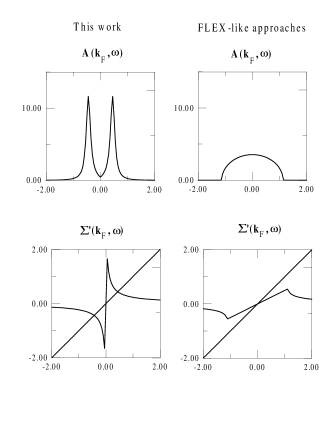
FIG. 11.: Top two panels are qualitative sketches of the spectral weight at the Fermi wave vector at half-filling. The plots are obtained by retainig only the classical contribution to the self-energy for $T<T_{X}$ using parameters corresponding to the typical $U=4$, of Monte Carlo simulations. The two bottom panels are the corresponding plots of $Re\Sigma(\omega)$. The left-hand side of this figure is obtained using our approximation while the right-hand side is obtained from the FLEX-like approach. The intersection with the $45$ degree line $\omega$ in the bottom-left panel gives rise to the precursors of antiferromagnetic bands seen right above it.

We now explain analytically the origin of these qualitative differences in the two theories. In our theory $\partial\Sigma^{\prime}({\bf k}_{F},\omega)/\partial\omega|_{\omega=0}\propto T\xi^{2}$and hence it quickly becomes larger than unity in the renormalized classical regime $\xi\propto\exp(const/T)$. In addition, for $\omega>v_{F}\xi^{-1}$the real part of the self-energy has the same behavior as in the ordered state $\Sigma({\bf k}_{F},\omega)\propto\Delta^{2}/\omega$with $\Delta^{2}\propto T\ln\xi=const$. The important point is that this asymptotic behavior $\Sigma({\bf k}_{F},\omega)\propto\Delta^{2}/\omega$of the self-energy already sets in for $\omega\sim\Delta\gg v_{F}\xi^{-1}$. It is this property that leads to the appearance of the precursors of antiferromagnetic bands at $\omega=\pm\Delta$in a manner analogous to the appearance of the Hubbard bands in the strong coupling limit that is discussed in the previous subsection. Let’s now try to understand analytically what happens in the FLEX approximation. As in our theory, the main contribution to the self-energy in the strongly fluctuating regime comes from the zero-frequency term in the Matsubara sum in the equation for the self-energy (Eq.(54) in our theory and Eq.(E9) in FLEX). An upper bound of the effect of the critical spin fluctuations can be obtained by approximating $T\tilde{\chi}^{RPA}({\bf q},0)\propto\delta({\bf q})$. Then one immediately obtains the same expression for the self-energy as the one obtained in FLEX in the context of Hubbard bands Eq.(71). (The only difference is that the parameter $\Delta$ is now defined by the zero-frequency Matsubara contribution of $\tilde{\chi}^{RPA}({\bf q},0)$, rather than by the sum over all Matsubara frequencies.) As we have already discussed in the context of Hubbard bands, such a form for $\Sigma$ does not lead to the appearance of two new quasiparticle solution away from $\omega=0$ because the characteristic behavior $\Sigma({\bf k}_{F},\omega)\propto\Delta^{2}/\omega$ sets in too late, namely for $\omega\gg\Delta$. In addition, the slope of $\Sigma^{\prime}\left({\bf k}_{F},\omega\right)$ at $\omega\rightarrow 0$ does not diverge with decreasing temperature as in our theory but instead saturates to its value given by the analog of Eq.(73), i.e. $\partial\Sigma^{\prime}\left({\bf k}_{F},\omega\right)/\partial\omega<1/2$. As we mentioned above, a value larger than unity $\partial\Sigma^{\prime}\left({\bf k}_{F},\omega\right)/\partial\omega>1$ would guarantee the existence of two new solutions of the quasiparticle equation Eq.(75) away from $\omega=0$. The right-hand side of Fig.(11) illustrates clearly what happens in a FLEX-like approach such as Eq.(71). The contribution of classical fluctuations to the spectral weight does not lead to a Fermi liquid since $A\left({\bf k}_{F},\omega\right)$ saturates to a finite width as temperature decreases, but nevertheless precursors of shadow bands do not occur because $\partial\Sigma^{\prime}\left({\bf k}_{F},\omega\right)/\partial\omega$ is bounded below unity. (Note that the spectral weight would not vanish so steeply at large frequencies if we had taken into account the quantum contribution of the spin fluctuations, as in full FLEX calculations.)

We just saw that the self-consistency in the propagators without corresponding self-consistency in the vertices inhibits the existence of the shadow bands in essentially the same way as it inhibits the existence of the Hubbard bands. It thus seems to us very likely that the absence of the precursors of antiferromagnetic bands below $T_{X}$ in FLEX is an artifact. This conclusion can be reliably verified by comparison with Monte Carlo data despite the fact that the latter is done for finite lattices and in the Matsubara formalism. This was discussed in more detail in Sec.(V B). Here we just note that the temperature dependence of Matsubara quantities such as $G({\bf k}_{F},\tau=\beta/2)$ and $\Sigma({\bf k}_{F},ik_{1})$ have a very characteristic form in the pseudogap regime. For example, $\Sigma({\bf k},ik_{1})\propto 1/(i\pi T)$ in the pseudogap regime, while in FLEX we would expect a much weaker temperature dependence of this quantity (the upper bound being given by the analog of Eq.(72)).

We also would like to comment on the 1D model[75] which describes the interaction of electrons with static spin fluctuations characterized by the susceptibility $\chi_{sp}\propto\delta(\omega)[\xi^{-1}/({\bf q}-{\bf Q})^{2}+\xi^{-2}]$. The nice thing about this model is that it has an exact solution which shows the development of shadow bands and of the pseudogap in $A\left({\bf k}_{F},\omega\right)$. A treatment similar to ours which uses non-interacting Green’s functions in the one-loop approximation also reproduces this feature[75]. However, the analogous approximation with dressed Green’s functions leads to Eq.(71) and hence inhibits the existence of the “shadow bands” and of the pseudogap in $A\left({\bf k}_{F},\omega\right)$.

In closing we comment on semantics and on the physical interpretation of some results obtained in the FLEX approximation. The expression “conserving approximation” has been widely used to describe FLEX calculations of the single particle properties and, in particular, in the context of the shadow bands and of the failure of Luttinger’s theorem [38, 37, 69]. The conserving aspect has been emphasized, but in fact the only desirable feature in the calculation of the single-particle properties is that the self-energy $\Sigma$ is obtained from a functional derivative of the Luttinger-Ward functional $\Sigma=\delta\Phi/\delta G$ and hence it is guaranteed to satisfy Luttinger’s theorem whenever appropriate. Only on the next level does this scheme lead to a calculation of the “true” susceptibilities[24] and of collective modes that satisfy conservation laws (Ward identities). However, these “true” susceptibilities are never substituted back in the calculation of the self-energy and the effect of “true” collective modes on the single-particle spectrum is an open question in FLEX. In fact, the RPA propagators $\tilde{\chi}_{RPA}$ appearing in the self-energy expression are different from susceptibilities from which collective modes should be computed and further they explicitly break conservation laws, as can be seen from the fact that RPA-like expressions $\tilde{\chi}_{RPA}=\tilde{\chi}_{0}/(1-U\tilde{\chi}_{0})$ with a dressed bubble $\tilde{\chi}_{0}$ have the unphysical properties that are mentioned in Eqs.(A26) and (A27) of Appendix (A). The fact that there are in effect two susceptibilities in the FLEX approximation leads, in our opinion, to some confusion and incorrect physical interpretation of the results in the literature. In particular, it was argued that the non-Fermi-liquid behavior and deviations from Luttinger theorem found in FLEX [38, 37, 69] are not due to critical thermal fluctuation in the vicinity of the phase transition but are rather the result of large $U$. The reasoning for such claim was that although the RPA susceptibilities $\tilde{\chi}_{RPA}$ is very strongly peaked at ${\bf q}={\bf Q}$, the “true” FLEX susceptibility is not. In our opinion, such claim could be justified only if one would substitute the “true” susceptibility back in the calculation of $\Sigma$ (for example using the exact Eq.(31)) and found that the deviation from the Luttinger theorem and other qualitative changes in $A(\vec{k},\omega)$ increase with decreasing temperature without almost divergent behavior of the conserving susceptibility $\chi_{sp}({\bf Q},0)$ and of the static structure factor $S_{sp}\left({\bf Q}\right).$

The Monte Carlo data on Fig.(7) are also instructive since they clearly show that qualitative changes in the single-particle spectra occur when the system enters the renormalized classical regime with rapidly growing $S_{sp}\left({\bf Q}\right)$. The fact that the FLEX “true” susceptibility does not show such behavior at half-filling[38] tells us that it even more drastically disagrees with the Monte Carlo data than the RPA-like $\tilde{\chi}$ which enters the expression for self-energy. Moreover, even away from half-filling the “true” susceptibility in FLEX at ${\bf q}={\bf Q}$ significantly underestimates the strength of the spin fluctuations, as is clear from the comparison with Monte Carlo data in Fig.(5). In our opinion the, so-called, “true susceptibility” in FLEX is the key element in the confusion surrounding the interpretation of FLEX results for the self-energy because the “true susceptibility” never comes in the calculation of the self-energy. For all practical purposes these calculations of the self-energy should be considered as consistent with Luttinger’s theorem at $T=0$ but based on a non-conserving susceptibility. Consistency with conservation laws and consistency with Luttinger’s theorem are not identical requirements because to satisfy rigorously Luttinger’s theorem one needs that $\Sigma=\delta\Phi/\delta G$, while to have conserving susceptibilities one needs that the irreducible vertices used in Bethe-Salpeter equation Eq.(26) should be obtained from $\Gamma=\delta^{2}\Phi/\delta G\delta G$.

VII Domain of validity of our approach

Our approach is not valid beyond intermediate coupling. That is perhaps best illustrated by Fig.(3) that shows that the crossover temperature first increases with $U$ and then saturates instead of decreasing. The decrease is expected on general grounds from the fact that at strong coupling the tendency to antiferromagnetism should decrease roughly as $J\sim t^{2}/U.$ The reason for this failure of our approach is clear. As we know from studies in infinite dimension[11], to account for strong-coupling effects it is necessary to include at least a frequency dependence to the self-energy and to the corresponding irreducible vertices.

Our theory also fails at half-filling deep in the renormalized classical regime, i.e. $T\ll T_{X}$ mainly for two reasons. First, the ansatz $U_{sp}=Ug_{\uparrow\downarrow}(0)$, Eq.(40), fails in the sense that $g_{\uparrow\downarrow}(0)$ eventually reaches zero at $T\rightarrow 0$ because of the $\log^{2}T$ divergence in the irreducible susceptibility $\chi_{0}\left(\pi,\pi\right)$ due to perfect nesting. The physically appropriate choice for $g_{\uparrow\downarrow}(0)$ in the renormalized classical regime is to keep its value fixed to its crossover-temperature value (See Fig.(6) and Sec.(IV)). The more serious reason why our approach fails for $T\ll T_{X}$ is that, as we just saw, critical fluctuations destroy completely the Fermi liquid quasiparticles and lead to a pseudogap. This invalidates our starting point. It is likely that in a more self-consistent theory, the logarithmic divergence of the appropriate irreducible susceptibility will be cutoff by the pseudogap. However, just a simple dressing of the Green’s function is not the correct solution to the problem because it would make the theory non-conserving, as we discussed in Sec.(A 3). One needs to take into account wave vector and energy dependent vertex corrections similar to those discussed by Schrieffer[76][77].

VIII Comparisons with other approaches

In Appendix (E), we discuss in detail various theories, pointing out limitations and advantages based on the criteria established in Appendix(A 2) and (A 3). More specifically, we include in our list of desirable properties, the local Pauli principle $\left\langle n_{\uparrow}^{2}\right\rangle=\left\langle n_{\uparrow}\right\rangle,$ the Mermin-Wagner theorem Eq.(A17), the Ward identities Eq.(A31), and $f-$sum rule Eq.(A25), one-particle vs two-particle consistency $\Sigma_{\sigma}\left(1,\overline{1}\right)G_{\sigma}\left(\overline{1},1^{+}\right)=U\left\langle n_{\uparrow}n_{\downarrow}\right\rangle$ Eq.(44), Luttinger’s theorem, and the large frequency asymptotic for the self-energy Eq.(68), which is important for the existence of the Hubbard bands. Comments on the forward scattering sum-rule Eq.(A36) appear in Appendix (A 4). In the present section, we only state without proof where each theory has strengths and weaknesses.

In standard paramagnon theories,[46][32] the spin and charge fluctuations are computed by RPA, using either bare or dressed Green’s functions. Then the fluctuations are feedback in the self-energy. When RPA with bare Green’s functions are used for the collective modes, these satisfy the $f-$sum rule, but that is the only one of our requirements that is satisfied by such theories.

In conserving approximation schemes[26],[24] the Mermin-Wagner theorem, the Luttinger theorem and conservation laws are satisfied, but none of the other above requirements are fulfilled.

In the parquet approach,[25][53] one enforces complete antisymmetry of the four point function by writing down fully crossing-symmetric equations for these. However, in actual calculations, the local Pauli principle, the Mermin Wagner theorem, and the consistency between one and two particle properties are only approximately satisfied, while nothing enforces the other requirements.

In our approach, the high-frequency asymptotics and Luttinger’s theorem are satisfied to a very good degree of approximation while all other properties in our list are exactly enforced. Let us specify the level of approximation. Luttinger’s theorem is trivially satisfied with our initial approximation for the self-energy $\Sigma_{\sigma}^{\left(0\right)},$ but at the next level of approximation, $\Sigma_{\sigma}^{\left(1\right)}$, one needs a new chemical potential to keep the electron density $Tr\left[G_{\sigma}^{\left(1\right)}\left(1,1^{+}\right)\right]$ fixed. With this new chemical potential the Fermi surface volume is preserved to a very high accuracy. Finally, consider the high-frequency asymptotics. Since we use bare propagators, the high-frequency asymptotics comes in at the appropriate frequency scale, namely $ik_{n}\sim W$, which is crucial for the existence of the Hubbard bands. However, the coefficient of the $1/ik_{n}$ term in the high-frequency expansion Eq.(68) is incorrect because our irreducible vertices $U_{sp}$ and $U_{ch}$ are tuned to the low frequencies. If one would take into account the frequency dependence of $U_{sp}$ and $U_{ch}$ and assume that at high frequency they become equal to the bare interaction $U$, then one would recover the exact result, provided the Pauli principle in the form of Eq.(39) is satisfied. The difficulty with such a procedure is that frequency dependent irreducible vertices requires frequency dependent self-energy in the calculation of collective modes and that would make the theory much more complicated. Yet it is, probably, the only way to extend the theory to strong coupling.

IX Conclusion

We have presented a new simple approach[29][30] to the repulsive single-band Hubbard model. We have also critically compared competing approaches, such as paramagnon, fluctuation exchange approximation, and pseudo-potential parquet approaches. Our approach is applicable for arbitrary band structure[34] and gives us not only a quantitative description of the Hubbard model, but also provide us with some qualitatively new results. Let us summarize our theory again. We first obtain spin and charge fluctuations by a self-consistent parameterization of the two-particle effective interactions (irreducible vertices) that satisfies a number of exact constraints usually not fulfilled by standard diagrammatic approaches to the many-body problem. Then the influence of collective modes on single-particle properties is taken into account in such a way that single-particle properties are consistent with two-particle correlators, which describe these collective modes. More specifically, our approach satisfies the following constraints:

1. Spin and charge susceptibilities, through the fluctuation-dissipation theorem, satisfy the Pauli principle in the form $\left\langle n_{\uparrow}^{2}\right\rangle=\left\langle n_{\uparrow}\right\rangle$ as well as the local moment sum-rule, conservations laws and consistency with the equations of motion in a local-field-like approximation.

2. In two dimensions, the spin fluctuations satisfy the Mermin-Wagner theorem.

3. The effect of collective modes on single-particle properties is obtained by a paramagnon-like formula that is consistent with the two-particle properties in the sense that the potential energy obtained from $Tr\left[\Sigma G\right]$ is identical to that obtained from applying the fluctuation-dissipation theorem to spin and charge susceptibilities.

4. Vertex corrections are included not only in spin and charge susceptibilities $\left(U_{sp}\neq U_{ch}\neq U\right)$ but also in the self-energy formula. In the latter case, this takes into account the fact that there is no Migdal theorem controlling the effect of spin and charge fluctuations on the self-energy.

The results for both single-particle and two-particle properties are in quantitative agreement with Monte Carlo simulations for all fillings, as long as $U$ is less than the bandwidth and $T$ is not much smaller than the crossover temperature $T_{X}$ where renormalized-classical behavior sets in. Both quantum-critical and renormalized-classical behavior can occur in certain parameter ranges but the critical behavior of our approach is that of the $O\left(n\right)$ model with $n\rightarrow\infty$.[33]

The main predictions of physical significance are as follows:

1. The theory predicts a magnetic phase diagram where magnetic order persists away from half-filling but with completely suppressed ferromagnetism.

2. In the renormalized classical regime above the zero-temperature phase transition, precursors of antiferromagnetic bands (shadow bands) appear in $A\left({\bf k}_{F},\omega\right)$. These precursors occur when $\xi>\xi_{th}$ (or $\omega_{SF}<T$). Between these precursors of antiferromagnetic bands a pseudogap appears at half-filling, so that the Fermi liquid quasiparticles are completely destroyed in a wide temperature range above the zero-temperature phase transition $0<T<T_{X}$. The upper critical dimension for this phenomenon is three. We stress the qualitative difference between the Hubbard bands and the precursors of antiferromagnetic bands and we predict that in two dimensions one may see both sets of bands simultaneously in certain parameter ranges. This prediction is consistent with the results of numerical simulations.[78][68]. We know of only one other analytic approach[70] which leads to similar four peak structure in the spectral function.

The zero temperature magnetic phase diagram is partly an open question because, despite the qualitative agreement with other analytical approaches, there is still an apparent contradiction with Monte Carlo simulations[64]. Our prediction of precursors of antiferromagnetic bands on the other hand is in agreement with Monte Carlo simulations. Neither this effect nor upper and lower Hubbard bands are observed in self-consistent schemes such as FLEX. This is because of inconsistent treatment of the vertex and self-energy corrections in this approximation, as we have explained in Sec.(VI). However, if there was a Migdal theorem for spin fluctuations, it would be justifiable to neglect the vertex corrections and keep only the self-energy effects as is done in the FLEX approximation. The presence of precursors of antiferromagnetic bands in two-dimensions is then a clear case of qualitatively new Physics that would not appear if there was a Migdal theorem for spin fluctuations. The same is true for the Hubbard bands for large $U>W$ in any dimension.

We would like to state again clearly the nature of our critique of approximation schemes which are based on using Migdal’s theorem for systems with electron-electron interactions. We do not imply that one does not need at all to take into account the feedback of the single-particle spectra on collective modes. The only point that we want to make here is that, based on sum rules and comparison with Monte Carlo data, we see that frequency and momentum dependent corrections to the self-energy and to the vertex often tend to cancel one another and that ignoring this leads to qualitatively incorrect results, in particular, with regards to the pseudogap. In this paper we were able to look only at the beginning of the renormalized classical regime when the pseudogap starts to form. The truly self-consistent treatment of the one-particle and two-particle properties in the pseudogap regime remains an open and very challenging problem. We hope that by extending our approach to the ordered state and looking at how the pseudogap starts to disappear as the temperature is raised, one can better understand how to develop a more self-consistent theory in the pseudogap regime. We now point out how our approach can be extended in other directions.

As we mentioned in Sec.(V), the pseudogap and precursors of antiferromagnetic bands in the two-dimensional repulsive Hubbard model have interesting analogs in the attractive Hubbard model. In that model, one expects a pairing pseudogap and precursors of superconducting quasiparticle bands above $T_{c}$. At half-filling the negative and positive Hubbard models are mapped onto one another by a canonical transformation and the present theory is directly applicable to the attractive case. However, away from half-filling the mapping between the two models is more complicated and the microscopic theory requires additional sum-rule for pairing susceptibilities to find self-consistently the effective pairing interaction. This work is now in progress.

The present approach can be also extended to stronger coupling $U>W$. Again the key idea would be to parameterize the irreducible vertices, which have now to be frequency dependent, and then use the most important sum-rules to find the parameterization coefficients. This will, of course, require solving much more complicated self-consistent equations than in the present approach, but we believe that the problem still can be made tractable.

Finally, we would like to make two comments about the magnetic and the pairing pseudogap in the context of high-$T_{c}$ superconductors, based on the results of our studies. First, as was stressed in Ref.[36], to understand clearly the physics of the single-particle pseudogap phenomena it is important to distinguish static short-range order from dynamical short-range order. The former is defined by a nearly Lorentzian form of the corresponding static structure factor $S({\bf q})\propto 1/(({\bf q}-{\bf Q})^{2}+\xi^{-2})$ (${\bf Q}=(\pi,\pi)$ in magnetic case, ${\bf Q}=0$ in the case of pairing), while the latter means only that the corresponding susceptibility $\chi({\bf q},0)$ has such a Lorentzian form. A condition for the existence of the single particle pseudogap in the vicinity of a given phase transition is that the corresponding short-range order is quasi-static (i.e.$~{}\omega_{SF}\ll T$)[36]. Experimentally, one can measure directly the dynamical spin structure factor $S({\bf q},\omega)$, and then obtain the static structure factor through the integral $S({\bf q})=\int S({\bf q},\omega)d\omega/(2\pi)$. Even if the zero-frequency dynamical structure factor $S_{sp}({\bf q},0)$ is very strongly peaked at ${\bf q}\sim{\bf Q}$ it is possible that the static structure factor $S_{sp}({\bf q)}$ is only weakly momentum dependent[36]. Thus in order to know whether one should expect to see the precursors of the antiferromagnetic bands and the corresponding pseudogap at a given doping and temperature it is necessary to obtain the static spin structure factor from the experimentally determined dynamical structure factor and then analyze its momentum dependence to see both if it is peaked and if it is quasi-two-dimensional.

The second comment that we would like to make is that both the pairing and the magnetic single-particle pseudogap discussed above are an effect of low dimensionality and hence they exist as long as there is a large two-dimensional fluctuating regime before the real three-dimensional phase transition. In this context, a pairing pseudogap could exist on either side of optimal doping.[79] The much larger temperature range over which a pseudogap appears in the underdoped compounds suggests that, in addition to pairing fluctuations, other thermal fluctuations (charge, spin…) prohibit finite-temperature ordering.[80] An example of this occurs in the attractive Hubbard model where charge fluctuations push the Kosterlitz-Thouless temperature to zero at half-filling, precisely where the crossover temperature to the pseudogap regime is largest.

We thank A.E. Ruckenstein, Liang Chen and R. Côté for helpful discussions and A. Georges for pointing out useful references. This work was partially supported by the Natural Sciences and Engineering Research Council of Canada (NSERC), the Fonds pour la formation de chercheurs et l’aide à la recherche from the Government of Québec (FCAR), and (for Y.M.V.) the National Science Foundation (Grant No. NSF-DMR-91-20000) through the Science and Technology Center for Superconductivity and (for A.-M.S.T.) the Killam Foundation as well as the Canadian Institute for Advanced Research (CIAR). A.-M.S.T. would like to thank the Institute for Theoretical Physics, Santa Barbara for hospitality during the writing of this work. Partial support there was provided by the National Science Foundation under Grant No. PHY94-07194.

A Sum rules, Ward identities and Consistency requirements

In this Appendix, we recall well known constraints on many-body theory that follow from sum-rules and conservation laws and comment, wherever possible, on their physical meaning and on where commonly used approaches fail to satisfy these constraints. Although we come back on a detailed discussion of various theories in a later appendix, we find it useful to include some of this discussion here to motivate our approach. We consider in turn various results that would be satisfied by any exact solution of the many-body problem. They are all consequences of either anticommutation relations alone (Pauli principle) or of anticommutation relations and the Heisenberg equations of motion. We describe in turn: 1. The relation between self-energy and two-body correlation functions that embodies the details of the Hamiltonian; 2. Sum rules for one-particle properties; 3. Sum rules and constraints on two-particle properties, in particular f-sum rule and Ward identities that express conservation laws; 4. A few relations that are crucial in Fermi liquid theory, namely Luttinger’s theorem and the forward scattering sum rule.

1 Equations of motion and the relation between the self-energy $\Sigma$ and two-particle properties.

The self-energy (we always mean one-particle irreducible self-energy) is related to the potential energy, and hence to two-particle correlations through the expression Eq.(44), which in the Kadanoff and Baym notation can be written as

$$\Sigma_{\sigma}\left(1,\overline{1}\right)G_{\sigma}\left(\overline{1},1^{+}\right)=U\left\langle n_{\uparrow}n_{\downarrow}\right\rangle.$$ (A1)

Here, the index with an overbar, $\overline{1},$ means that there is a sum over corresponding lattice positions and an integral over imaginary time. The notation $1^{+}$ means that the imaginary time implicit in $1$ is $\tau_{1}+\eta$ where $\eta$ is a positive infinitesimal number. Eq.(A1) is an important consistency requirement between self-energy and double occupancy in the Hubbard model that can easily be proven as follows. From the equations of motion for the single-particle Green’s function Eq.(3) one finds,

$\displaystyle\left[\left(-\frac{\partial}{\partial\tau_{i}}+\mu\right)\delta_{i,\ell}+t_{i\ell}\right]G_{\sigma}\left({\bf r}_{\ell}-{\bf r}_{j},\tau_{i}-\tau_{j}\right)$

$$=\delta_{i,j}\delta\left(\tau_{i}-\tau_{j}\right)-U\left\langle T_{\tau}\left(c_{i-\sigma}^{\dagger}\left(\tau_{i}\right)c_{i-\sigma}\left(\tau_{i}\right)c_{i\sigma}\left(\tau_{i}\right)c_{j\sigma}^{\dagger}\left(\tau_{j}\right)\right)\right\rangle.$$ (A2)

Using the short-hand notation in Eqs.(3) and (4) and the definition of self-energy (Dyson’s equation) the above equation is also written in the form,

$$G_{0}^{-1}\left(1,\overline{1}\right)G_{\sigma}\left(\overline{1},2\right)=\delta\left(1-2\right)+\Sigma_{\sigma}\left(1,\overline{1}\right)G_{\sigma}\left(\overline{1},2\right).$$ (A3)

Comparing the last two equations, the well known relation Eq.(A1) (or Eq.(44)) between self-energy, Green’s function and potential energy follows.

So-called conserving[26] approaches to the many-body problem violate the above consistency requirement Eq.(44) in the following sense. The right-hand side can be computed from the collective modes using the fluctuation-dissipation theorem. In conserving approximations, this gives a result that is different from what is computed directly from the left-hand side of the equation, namely from the self-energy and from the Green’s function. In fact, all many-body approaches satisfy the above consistency requirement at best in an approximate way. However, it is a very important requirement and Eq.(44) plays a key role in our discussion. Seen in Matsubara frequency, it is a sum rule, or an integral constraint that involves all frequencies, large and small.

2 Constraints on single-particle properties:

The spectral weight $A_{\sigma}\left({\bf k},\omega\right)$ can be interpreted as a probability of having an electron in a state $\left(\sigma,{\bf k},\omega\right)$ and it satisfies the normalization sum rule

$$\int_{-\infty}^{\infty}\frac{d\omega}{2\pi}A_{\sigma}\left({\bf k},\omega\right)=\left\langle\left\{c_{{\bf k}\sigma},c_{{\bf k}\sigma}^{\dagger}\right\}\right\rangle=1.$$ (A4)

Formally this is a consequence of the jump in the Green’s function at $\tau=0$, as can be seen from calculating

$$G_{\sigma}\left({\bf k},0^{-}\right)-G_{\sigma}\left({\bf k},0^{+}\right)=1=T\sum_{ik_{n}}\left(e^{ik_{n}\eta}-e^{-ik_{n}\eta}\right)\int_{-\infty}^{\infty}\frac{d\omega}{2\pi}\frac{A_{\sigma}\left({\bf k},\omega\right)}{ik_{n}-\omega}=\int_{-\infty}^{\infty}\frac{d\omega}{2\pi}A_{\sigma}\left({\bf k},\omega\right).$$ (A5)

To do perturbation theory directly for the Green’s function to any finite order would require that the interaction $U$ be small not only in comparison with the bandwidth $W$ but also in comparison with the smallest Matsubara frequency $ik_{1}=2\pi T$. Also, the direct perturbation series for the Green’s function gives, after analytical continuation, poles of arbitrary high order located at the unperturbed energies. These high-order poles are inconsistent with the simple pole (or branch cut) structure of the Green’s function predicted by the spectral representation. Furthermore, the high-order poles lead to a spectral weight that can be negative.[81] The common way to get around these difficulties is to make approximations for the self-energy $\Sigma$ instead and then calculate the Green’s function using Dyson’s equation Eq.(8).

It is interesting to note that to satisfy the constraint Eq.(A4), it suffices that $\Sigma({\bf k},ik_{n})$, defined by Eq.(8), has a finite limit as $ik_{n}\rightarrow\infty.$ More constraints on approximations for the self-energy may be found by continuing this line of thought. A systematic way of doing this is to do a high-frequency expansion for both the Matsubara Green’s function and the self-energy and to find coefficients using sum-rules. The sum-rules that we need then are[82]

$$\int_{-\infty}^{\infty}\frac{d\omega}{2\pi}\omega A_{\sigma}\left({\bf k},\omega\right)=\left\langle\left\{\left[c_{{\bf k}\sigma},\left(H-\mu N\right)\right],c_{{\bf k}\sigma}^{\dagger}\right\}\right\rangle=\epsilon_{{\bf k}}-\mu+Un_{-\sigma}$$ (A6)

$$\int_{-\infty}^{\infty}\frac{d\omega}{2\pi}\omega^{2}A_{\sigma}\left({\bf k},\omega\right)=(\epsilon_{{\bf k}}-\mu)^{2}+2U(\epsilon_{{\bf k}}-\mu)n_{-\sigma}+U^{2}n_{-\sigma}$$ (A7)

where $n_{\sigma}=n/2$ since we are in the paramagnetic state.

Using the spectral representation Eq.(6) one can easily see that the above sum rules give the coefficients of the high-frequency expansion of the Matsubara Green’s function

$$\lim_{ik_{n}\rightarrow\infty}G_{\sigma}\left({\bf k,}ik_{n}\right)=\frac{1}{ik_{n}}+\left(\frac{1}{ik_{n}}\right)^{2}\int\frac{d\omega}{2\pi}\omega A_{\sigma}\left({\bf k},\omega\right)+\left(\frac{1}{ik_{n}}\right)^{3}\int\frac{d\omega}{2\pi}\omega^{2}A_{\sigma}\left({\bf k},\omega\right)+\ldots$$ (A8)

The self-energy has the same analytic properties as the Green’s function. Using its high frequency expansion in the expression for the Green’s function Eq.(8), one finds that the first term in Eq.(A8), leads to the requirement that the self-energy has a finite limit at $ik_{n}\rightarrow\infty$. The second term fixes the value of this constant to the Hartree-Fock result, and the last and second-term combine to give the leading term in $1/ik_{n}\$of the self-energy high-frequency expansion. In short, we find the result quoted in Eq.(68), namely

$$\lim_{ik_{n}\rightarrow\infty}\Sigma_{\sigma}\left({\bf k,}ik_{n}\right)=Un_{-\sigma}+\frac{U^{2}n_{-\sigma}\left(1-n_{-\sigma}\right)}{ik_{n}}+\ldots$$ (A9)

The Kramers-Kronig relation for the self-energy

$$\mathop{\rm Re}\left[\Sigma_{\sigma}^{R}\left({\bf k,}\omega\right)-\Sigma_{\sigma}^{R}\left({\bf k,}\infty\right)\right]={\cal P}\int\frac{d\omega^{\prime}}{\pi}\frac{\mathop{\rm Im}\left[\Sigma_{\sigma}^{R}\left({\bf k,}\omega^{\prime}\right)\right]}{\omega^{\prime}-\omega}.$$ (A10)

and the high-frequency result Eq.(A9) imply the following sum-rule for the imaginary part of the self-energy

$$-\int\frac{d\omega^{\prime}}{\pi}\mathop{\rm Im}\left[\Sigma_{\sigma}^{R}\left({\bf k,}\omega^{\prime}\right)\right]=U^{2}n_{-\sigma}\left(1-n_{-\sigma}\right)$$ (A11)

Important consequences of this equation are that for a given $U$ the integrated imaginary part of the self-energy is independent of temperature and is increasing towards half-filling. The right-hand side of this equation is also a measure the width of the single-particle excitation spectrum, as can be seen from the spectral weight moments Eqs.(A6) and (A7),

$$\overline{\omega^{2}}-\overline{\omega}^{2}\equiv\int_{-\infty}^{\infty}\frac{d\omega}{2\pi}\omega^{2}A_{\sigma}\left({\bf k},\omega\right)-\left[\int_{-\infty}^{\infty}\frac{d\omega}{2\pi}\omega A_{\sigma}\left({\bf k},\omega\right)\right]^{2}=U^{2}n_{-\sigma}\left(1-n_{-\sigma}\right)$$ (A12)

An important physical point is that the asymptotic behavior Eq.(A9) is a necessary condition for the existence of upper and lower Hubbard bands, as has been explained in Sec.VI A. However, it is important to realize that it is not a sufficient condition. Indeed, the following paradox has been noticed in explicit calculations in infinite dimensions[74],[11]. While ordinary second-order perturbation theory with bare Green functions $G_{0\text{ }}$reproduces correctly the appearance of the Hubbard bands with increasing $U$, the perturbation theory with dressed Green function $G=[G_{0\text{ }}^{-1}-\Sigma]^{-1}$ does not. The reason for this is that although the second-order expression for $\Sigma_{\sigma}\left({\bf k,}ik_{n}\right)$ in terms of full $G$ does satisfy the asymptotics Eq.(A9), it sets in too late, namely for $k_{n}\gg U$, instead of $k_{n}\gg W$. The fact that the asymptotics should start at $k_{n}\sim W$ even when $U>W$ is a non-trivial consequence of the Pauli principle, as explained in Sec.(VI A). Thus there are no Hubbard bands in any theory that uses self-consistent Green functions but neglects the frequency dependence of the vertex. This is an explicit example that illustrates what seems to be a more general phenomena: a calculation with dressed Green’s functions but no frequency dependent vertex correction often gives worse results that the one done with bare Green’s functions and a frequency independent vertex. We will see in the next subsection that this also happens in the calculation of the two-particle properties. Also, as we have argued in Sec.(VI), a similar situation occurs with the precursors of antiferromagnetic bands in the renormalized classical regime in two-dimensions.

Finally, we quote two more well known sum-rules that we will need. They involve the Fermi function $f\left(\omega\right)$ and the spectral weight. The first one follows from definition of $G_{\sigma}\left({\bf k,}\tau\right)$ and the spectral representation

$$\lim_{\tau\rightarrow 0^{-}}G_{\sigma}\left({\bf k,}\tau\right)=\int\frac{d\omega}{2\pi}f\left(\omega\right)A_{\sigma}\left({\bf k,}\omega\right)=\left\langle c_{{\bf k}\sigma}^{\dagger}c_{{\bf k}\sigma}\right\rangle\equiv n_{{\bf k}\sigma}.$$ (A13)

The quantity $n_{{\bf k}\sigma}$ is the distribution function. It is equal to the Fermi function only when the self-energy is frequency independent. The next result, that follows simply from the equations of motion,

$$\lim_{\tau\rightarrow 0^{-}}-\frac{1}{N}\sum_{{\bf k}}\frac{\partial G_{\sigma}\left({\bf k,}\tau\right)}{\partial\tau}=\frac{1}{N}\sum_{{\bf k}}\int\frac{d\omega}{2\pi}\omega f\left(\omega\right)A_{\sigma}\left({\bf k,}\omega\right)=\frac{1}{N}\sum_{{\bf k}}\left(\epsilon_{{\bf k}}-\mu\right)n_{{\bf k}\sigma}+U\left\langle n_{\uparrow}n_{\downarrow}\right\rangle$$ (A14)

is useful to show to what extent certain dressed-propagator approaches fail to satisfy the $f-$sum rule.

3 Constraints on two-particle properties

For any one-band model, independently of the Hamiltonian, the Pauli principle (anticommutation relations)

$$\left\langle n_{i\sigma}^{2}\right\rangle=\left\langle n_{i\sigma}\right\rangle$$ (A15)

implies the following two simple identities:

$$\left\langle\left(n_{i\uparrow}\pm n_{i\downarrow}\right)^{2}\right\rangle=n\pm 2\left\langle n_{i\uparrow}n_{i\downarrow}\right\rangle.$$ (A16)

The correlation functions on the left-hand side are equal-time and equal-position spin and charge correlation functions. The susceptibilities $\chi_{ch}\left({\bf r}_{i}-{\bf r}_{j},\tau\right),$ $\chi_{sp}\left({\bf r}_{i}-{\bf r}_{j},\tau\right)$ in Eqs.(17) and (16) are response functions for arbitrary $\left({\bf r}_{i}-{\bf r}_{j},\tau\right)$ so they must reduce to the above equal-time equal-position correlation functions when ${\bf r}_{i}={\bf r}_{j}$ and $\tau=0$. This is one special case of the imaginary-time version of the fluctuation-dissipation theorem Eqs.(16)(17). This translates into local-moment and local-charge sum-rules for the susceptibilities

$$\frac{T}{N}\sum_{{\bf q}}\sum_{iq_{n}}\chi_{sp}\left({\bf q},iq_{n}\right)=2\left\langle n_{\uparrow}n_{\uparrow}\right\rangle-2\left\langle n_{\uparrow}n_{\downarrow}\right\rangle=n-2\left\langle n_{\uparrow}n_{\downarrow}\right\rangle$$ (A17)

$$\frac{T}{N}\sum_{{\bf q}}\sum_{iq_{n}}\chi_{ch}\left({\bf q},iq_{n}\right)=2\left\langle n_{\uparrow}n_{\uparrow}\right\rangle+2\left\langle n_{\uparrow}n_{\downarrow}\right\rangle-n^{2}=n+2\left\langle n_{\uparrow}n_{\downarrow}\right\rangle-n^{2}$$ (A18)

where we have removed the $i$ dependence of $\left\langle n_{i\uparrow}n_{i\downarrow}\right\rangle$ using translational invariance. The right-hand side of the local-moment sum-rule is equal to $\left\langle\left(S^{z}\right)^{2}\right\rangle,$while that of the local-charge sum rule is equal to $\left\langle\rho^{2}\right\rangle-n^{2}$

If arbitrary sets of diagrams are summed, nothing can prevent the right-hand side from taking unphysical values. For example, the Pauli principle may be violated, i.e. $\left\langle n_{\uparrow}n_{\uparrow}\right\rangle\neq\left\langle n_{\uparrow}\right\rangle.$ To see this, notice that when the Pauli principle is satisfied, our two sum rules Eqs.(A17) and (A18) lead to

$$\frac{T}{N}\sum_{{\bf q}}\sum_{iq_{n}}\left[\chi_{sp}\left({\bf q},iq_{n}\right)+\chi_{ch}\left({\bf q},iq_{n}\right)\right]=2n-n^{2}.$$ (A19)

It is easy to check that well known approaches to the many-body problem, such as RPA, violate this basic requirement. Indeed, the ordinary RPA expressions for spin and charge are

$$\chi_{sp}^{RPA}(q)\equiv\frac{\chi_{0}}{1-\frac{U}{2}\chi_{0}}$$ (A20)

$$\chi_{ch}^{RPA}(q)\equiv\frac{\chi_{0}}{1+\frac{U}{2}\chi_{0}}$$ (A21)

where

$$\chi_{0}\left(q\right)=-2\frac{T}{N}\sum_{k}G^{\left(0\right)}\left(k\right)G^{\left(0\right)}\left(k+q\right).$$ (A22)

That RPA does not satisfy the sum rule Eq.(A19) already to second order in $U$ can be easily seen by expanding the denominators.

To satisfy the Mermin-Wagner theorem, approximate theories must also prevent $\left\langle n_{\uparrow}n_{\downarrow}\right\rangle$ from taking unphysical values. This quantity is positive and bounded by its value for $U=\infty$ and its value for non-interacting systems, namely $0\leq\left\langle n_{\uparrow}n_{\downarrow}\right\rangle\leq n^{2}/4$. Hence, the right-hand side of the local-moment sum-rule Eq.(A17) is contained in the interval $\left[n,n-\frac{1}{2}n^{2}\right].$ Any theory that prevents the right-hand side of the local-moment sum rule from taking infinite values satisfies the Mermin-Wagner theorem.

  Proof:

Near a magnetic phase transition, the zero Matsubara-frequency component of the spin susceptibility takes the Ornstein-Zernicke form

$$\chi_{sp}\left({\bf q+Q},0\right)\sim\frac{1}{q^{2}+\xi^{-2}}$$ (A23)

where $q$ is measured with respect to the ordering wave vector ${\bf Q}$ and where $\xi^{2}$ is the square of the correlation length. Near its maximum, the above susceptibility is of order $\xi^{2}$ while all finite Matsubara-frequency components at the ordering wave vector are at most of order $1/\left(2\pi T\right)^{2}$ which is much smaller than $\xi^{2}$. Hence, one can keep only the zero-Matsubara frequency contribution on the left-hand side of the local-moment sum rule Eq.(A17) obtaining

$$T\int\frac{d^{d}{\bf q}}{\left(2\pi\right)^{d}}\frac{1}{q^{2}+\xi^{-2}}=\widetilde{C}$$ (A24)

where $\widetilde{C}$ contains non-zero Matsubara frequency contributions as well as $n-2\left\langle n_{\uparrow}n_{\downarrow}\right\rangle.$ Since $\widetilde{C}$ is finite, this means that in two dimensions $\left(d=2\right)$, it is impossible to have $\xi^{-2}=0$ on the left-hand side otherwise the integral would diverge logarithmically.

Finally, the $f$-sum rule on spin and charge susceptibilities follows as usual from the fact that the Hamiltonian conserves particle number. Computing $\left.\left\langle\left[\rho_{{\bf q}},\frac{\partial\rho_{-{\bf q}}}{\partial\tau}\right]\right\rangle\right|_{\tau=0}$ and $\left.\left\langle\left[S_{{\bf q}},\frac{\partial S_{-{\bf q}}}{\partial\tau}\right]\right\rangle\right|_{\tau=0}$one obtains for either charge or spin

$$\int\frac{d\omega}{\pi}\omega\chi_{ch,sp}^{\prime\prime}\left({\bf q,}\omega\right)=\lim_{\eta\rightarrow 0}T\sum_{iq_{n}}\left(e^{-iq_{n}\eta}-e^{iq_{n}\eta}\right)iq_{n}\chi_{ch,sp}\left({\bf q},iq_{n}\right)=\frac{1}{N}\sum_{{\bf k}\sigma}\left(\epsilon_{{\bf k+q}}+\epsilon_{{\bf k-q}}-2\epsilon_{{\bf k}}\right)n_{{\bf k}\sigma}.$$ (A25)

As can be seen from the spectral representations of spin and charge susceptibilities, Eq.(20), the quantity that obeys the $f-$sum rule is the coefficient of the leading term in the $1/q_{n}^{2}$ high-frequency expansion of the susceptibilities.

The single-particle energies $\epsilon_{{\bf k}}$ entering explicitly the right-hand side of the $f-$sum rule are independent of interactions, so interactions influence the $f-$sum rule only very weakly through the $n_{{\bf k}\sigma}$. In fact, in a continuum $\epsilon_{{\bf k}}\propto{\bf k}^{2}$ so $n_{{\bf k}\sigma}$ enters only in the form $\sum_{{\bf k}\sigma}n_{{\bf k}\sigma}=n$ . In this case, the right-hand side of the $f-$sum rule is proportional to $q^{2}n$ and hence is independent of interactions. On a lattice however, the energies cannot in general be taken out of the sum and interactions influence the value of the right-hand side, but only through the fact that $n_{{\bf k}\sigma}$ differs from the non-interacting Fermi function $f_{{\bf k}\sigma}$. At strong-coupling, where the self-energy is strongly frequency dependent, this difference between $n_{{\bf k}\sigma}$ and $f_{{\bf k}\sigma}$ becomes important. But from weak to intermediate coupling, calculations where $f_{{\bf k}\sigma}$ appears on the right-hand side should be good approximations. In the explicit examples that we have treated, the $U$ dependence of the $f-$sum rule becomes important only close to half-filling and for $U>4$, signaling the breakdown of approximations based on frequency-independent self-energies.

While RPA-like theories that use $f_{{\bf k}\sigma}$ instead of $n_{{\bf k}\sigma}$ violate only weakly the $f-$ sum rule in the weak to intermediate coupling regime, self-consistent theories that use frequency-dependent self-energies but no frequency-dependent vertices violate conservations laws in general, and the $f-$ sum rule in particular, in a much more dramatic way. The point is that susceptibilities with a dressed bubble, $\tilde{\chi}_{RPA}=\tilde{\chi}_{0}/(1-\frac{1}{2}U\tilde{\chi}_{0}),$ are bad approximations because they have the following properties, for any value of $U$

$$\tilde{\chi}_{RPA}({\bf q}=0,iq_{n}\neq 0)\neq 0$$ (A26)

$$\int\frac{d\omega}{2\pi}\omega\tilde{\chi}_{RPA}^{\prime\prime}\left({\bf q,}\omega\right)=\frac{1}{N}\sum_{{\bf k,}\sigma}\left(\epsilon_{{\bf k+q}}+\epsilon_{{\bf k-q}}-2\epsilon_{{\bf k}}\right)n_{{\bf k}\sigma}+4U\left(\left\langle n_{\uparrow}\right\rangle\left\langle n_{\downarrow}\right\rangle-\left\langle n_{\uparrow}n_{\downarrow}\right\rangle\right).$$ (A27)

The first of these equations explicitly violates the Ward identity, Eq.(A31) below, at all frequencies, including small non-zero ones, since at zero wave vector we should have $\chi({\bf q}=0,iq_{n}\neq 0)=0$ for all frequencies except zero. The second equation, Eq.(A27) violates the $f$-sum rule Eq.(A25) at all wave vectors, by a constant term $4U\left(\left\langle n_{\uparrow}\right\rangle\left\langle n_{\downarrow}\right\rangle-\left\langle n_{\uparrow}n_{\downarrow}\right\rangle\right)$ which in practical calculations, say at $U=4$, is of the same order as the first term, which is the only one that should be there according to the $f$-sum rule.

  Proof:

Eqs.(A26) and (A27) are proven as follows. Consider the standard RPA expression but with dressed bubbles $\tilde{\chi}_{0}$

$$\tilde{\chi}_{RPA}=\tilde{\chi}_{0}/(1-\frac{U}{2}\tilde{\chi}_{0}).$$ (A28)

Using the spectral representation for the Green’s function and inversion symmetry in the Brillouin zone one finds,

$$\tilde{\chi}_{0}\left({\bf q},iq_{n}\right)=\frac{2}{N}\sum_{{\bf k}}\int\frac{d\omega}{2\pi}\int\frac{d\omega^{\prime}}{2\pi}A\left({\bf k,}\omega\right)A\left({\bf k+q,}\omega^{\prime}\right)\frac{\left(\omega-\omega^{\prime}\right)\left(f\left(\omega^{\prime}\right)-f\left(\omega\right)\right)}{\left(\omega-\omega^{\prime}\right)^{2}+q_{n}^{2}}.$$ (A29)

When the bubble is not dressed, the spectral weights are delta functions so that at ${\bf q}=0$ the susceptibility would vanish for all non-zero values of $q_{n}$, as required by the Ward identity. However, here because the spectral weight has a width and because the integrand is even and positive, then the integral will not vanish, resulting in the first anomaly Eq.(A26) we mention. To prove the second equation, Eq.(A27), it suffices to remember from the spectral representation of the susceptibility Eq.(20) and the derivation of the $f-$sum rule Eqs.(A25) that we are looking for the coefficient of the $1/q_{n}^{2}$ term in the high-frequency expansion. Given the RPA form, Eq.(A28), only the numerator contributes to this limit. One obtains, for the coefficient of the $1/q_{n}^{2}$ term,

$$\frac{2}{N}\sum_{{\bf k}}\int\frac{d\omega}{2\pi}\int\frac{d\omega^{\prime}}{2\pi}A\left({\bf k,}\omega\right)A\left({\bf k+q,}\omega^{\prime}\right)\left(\omega-\omega^{\prime}\right)\left(f\left(\omega^{\prime}\right)-f\left(\omega\right)\right)$$ (A30)

from which Eq.(A27) follows using the sum rules for occupation number Eq.(A13) and for energy (A14).

Conservation laws have general consequences not only on equal-time correlation functions, as in the $f-$sum rule above, but also on time-dependent correlation functions. For example, from the Heisenberg equations of motion and anti-commutation relations, follow the Ward identities[45]

$\displaystyle\sum_{{\bf k}}\sum_{\sigma=\pm 1}\sum_{\sigma^{\prime}=\pm 1}\left(\frac{\partial}{\partial\tau}+\left(\epsilon_{{\bf k+q}}-\epsilon_{{\bf k}}\right)\right)\left\langle T_{\tau}c_{{\bf k}\sigma}^{\dagger}\left(\tau\right)\sigma^{\ell}c_{{\bf k+q}\sigma}\left(\tau\right)c_{{\bf k}^{\prime}+{\bf q}\sigma^{\prime}}^{\dagger}\left(\tau_{1}\right)\sigma^{\prime\ell}c_{{\bf k}^{\prime}\sigma^{\prime}}\left(\tau_{2}\right)\right\rangle$

$$=\delta\left(\tau-\tau_{1}\right)\sum_{\sigma^{\prime}=\pm 1}\sigma^{\prime\ell}G_{\sigma^{\prime}}\left({\bf k}^{\prime},\tau_{2}-\tau\right)-\delta\left(\tau-\tau_{2}\right)\sum_{\sigma^{\prime}=\pm 1}\sigma^{\prime\ell}G_{\sigma^{\prime}}\left({\bf k}^{\prime}+{\bf q},\tau-\tau_{1}\right)$$ (A31)

where $\ell=0$ for charge, and $\ell=1$ for spin. The $f-$sum rule above, Eq.(A25), follows from the above identity by simply taking $\tau_{1}=\tau_{2}^{+}$, summing over ${\bf k}^{\prime}$ and subtracting the two results for $\tau\rightarrow\tau_{1}^{+}$ and $\tau\rightarrow\tau_{1}^{-}$.

We have seen in this section that there are strong cancelations for two-particle properties between the frequency dependence of self-energy and that of the vertex corrections, so that putting a frequency dependence in only one of them is a bad approximation. We have adopted the Kadanoff-Baym formalism in the main text since it can be used as a guide to make approximations that satisfy conservation laws.

4 When there is a Fermi surface

When perturbation theory converges (no phase transition) then at zero temperature $T=0$ the imaginary part of the self-energy vanishes, $\Sigma_{\sigma}^{\prime\prime}\left({\bf k,}\omega=0\right)=0$, for all ${\bf k}$ values and the Fermi surface defined by

$$\epsilon_{{\bf k}}-\mu-\Sigma_{\sigma}^{\prime}\left({\bf k,}\omega=0\right)=0$$ (A32)

encloses a volume that is equal to the volume enclosed by non-interacting particles

$$\frac{1}{N}\sum_{{\bf k}}\theta\left(\mu-\epsilon_{{\bf k}}-\Sigma_{\sigma}^{\prime}\left({\bf k,}0\right)\right)=\frac{1}{N}\sum_{{\bf k}}\theta\left(\mu_{0}-\epsilon_{{\bf k}}\right)=n_{\sigma}.$$ (A33)

This is the content of Luttinger’s theorem.[28][83]. It implies that there is a strong cancelation between the change of the chemical potential and the change of the self-energy on the Fermi surface. In particular, when $\Sigma_{\sigma}^{\prime}\left({\bf k}_{F}{\bf,}0\right)$ does not depend on ${\bf k}$ or on the direction of ${\bf k}_{F}$ (infinite $D$ Hubbard model, electron gas) the change in $(\mu-\mu_{0})$ is exactly canceled by $\Sigma_{\sigma}^{\prime}\left({\bf k}_{F}{\bf,}0\right)$

$$\mu-\mu_{0}=\Sigma_{\sigma}^{\prime}\left({\bf k}_{F}{\bf,}0\right).$$ (A34)

Luttinger’s theorem is satisfied when

$$\lim_{T\rightarrow 0}\int\frac{\partial\Sigma_{\sigma}\left({\bf k,}i\nu\right)}{\partial(i\nu)}G_{\sigma}\left({\bf k,}i\nu\right)d\nu d{\bf k}=0.$$ (A35)

Any theory that calculates its self-energy from a functional derivative of the Luttinger-Ward functional $\Sigma=\delta\Phi[G]/\delta G$ will satisfy Luttinger’s theorem[28][83]. The latter procedure requires self-consistent determination of the self-energy as a function of momentum and frequency $\Sigma_{\sigma}\left({\bf k,}ik_{n}\right)$ and is usually quite computationally involved. However, even when this procedure to calculate the self-energy is not followed, it turns out to be rather easy to satisfy this theorem to an excellent degree of approximation in the weak to intermediate coupling regime. The reason for this is that any frequency-independent self-energy will preserve Luttinger’s theorem and weak frequency dependence will not cause great harm. For the electron gas, Luttinger[28] suggests a way to build a perturbation theory in terms of non-interacting Green’s functions which allows to satisfy Luttinger’s theorem to very good accuracy. The trick is that the chemical potential for the interacting electrons $\mu$ should always enter the calculations in the form of the difference with the shift of the self-energy on the Fermi surface $\tilde{G}_{0}=1/[ik_{n}-\epsilon_{{\bf k}}+(\mu-\Sigma_{\sigma}^{\prime}\left({\bf k}_{F}{\bf,}0\right))]$. The “non-interacting” Green’s function $\tilde{G}_{0}$ in this formalism is the Green’s function of some effective non-interacting system and, in general, it is different from both $1/\left(ik_{n}-\epsilon_{{\bf k}}+\mu\right)$ and $1/\left(ik_{n}-\epsilon_{{\bf k}}+\mu_{0}\right)$. However, when $T\rightarrow 0$ Luttinger’s theorem requires that $(\mu-\Sigma_{\sigma}^{\prime}\left({\bf k}_{F}{\bf,}0\right))\rightarrow\mu_{0}$ and one can approximate $\tilde{G}_{0}$ by the Green’s function for a non-interacting system of the same density $G_{0}=1/\left(ik_{n}-\epsilon_{{\bf k}}+\mu_{0}\right)$. In practice, one can also have a phase transition (or crossover) at a finite temperature $T_{c}$ ($T_{X}$). In these cases Luttinger’s theorem is satisfied only approximately since the zero-temperature limit cannot be reached without a breakdown of perturbation theory. Then the relevant question is how well it is satisfied at $T_{c}$ ($T_{X}$). (See also Sec.(III B 2) for a discussion of Luttinger’s theorem in our approach)

When Luttinger’s theorem holds, one can usually develop a Landau Fermi liquid theory. In this approach, the Pauli principle is implemented only for momentum states near the Fermi surface by imposing the forward scattering sum rule. This sum rule, in two dimensions, reads

$$\sum_{\ell}\left[\frac{F_{\ell}^{s}}{1+F_{\ell}^{s}}+\frac{F_{\ell}^{a}}{1+F_{\ell}^{a}}\right]=0$$ (A36)

where $F_{\ell}^{s}$ and $F_{\ell}^{a}$ are the symmetric and antisymmetric Landau parameters expanded on the $e^{-i\theta\ell}$ basis instead of the Legendre polynomial basis. Recent renormalization group analysis has however claimed[84] that the forward scattering sum rule comes from an inaccurate use of crossing symmetry and is not the proper way to enforce the Pauli principle. Most approaches to the many-body problem disregard this sum rule anyway, in the same way that they disregard the local Pauli principle.

B Proofs of various formal results

In this appendix, we give the proofs of various relations mentioned in Secs.(III) and (III B 3).

1. The general expression for the self-energy Eq.(27) can be obtained as follows. Use the equations of motion and the definition of the self-energy Eqs.(A2)(A3) which in the present notation give

   $$\Sigma_{\sigma}\left(1,\overline{1}\right)G_{\sigma}\left(\overline{1},2\right)=-U\left\langle T_{\tau}\left[\psi_{-\sigma}^{+}\left(1^{++}\right)\psi_{-\sigma}\left(1^{+}\right)\psi_{\sigma}\left(1\right)\psi_{\sigma}^{+}\left(2\right)\right]\right\rangle$$ (B1)

   $$=-U\left[\frac{\delta G_{\sigma}\left(1,2\right)}{\delta\phi_{-\sigma}\left(1,1^{+}\right)}-G_{-\sigma}\left(1,1^{+}\right)G_{\sigma}\left(1,2\right)\right]$$ (B2)

   Substituting the equation for the three-point susceptibility (collective modes) Eq.(26) in this last equation and multiplying on both sides by $G^{-1}$ proves[27] the expression Eq.(27) for the self-energy.

2. We now show that our approach satisfies the consistency requirement between single-particle properties and collective modes in the form of Eq.(48). Using our expression Eq.(46) for $\Sigma^{\left(1\right)}$ and the definition of $\chi_{0}$ Eq.(A22) we obtain

   $$\lim_{\tau\rightarrow 0^{-}}\frac{T}{N}\sum_{k}\Sigma_{\sigma}^{\left(1\right)}\left(k\right)G_{\sigma}^{\left(0\right)}\left(k\right)e^{-ik_{n}\tau}=Un_{-\sigma}^{2}-\frac{U}{4}\frac{T}{N}\sum_{q}\left[U_{sp}\chi_{sp}(q)+U_{ch}\chi_{ch}(q)\right]\frac{\chi_{0}\left(q\right)}{2}$$ (B3)

   Using

   $$\chi_{sp}(q)-\chi_{0}\left(q\right)=\frac{U_{sp}}{2}\chi_{0}\left(q\right)\chi_{sp}(q)$$ (B4)

   $$\chi_{0}\left(q\right)-\chi_{ch}(q)=\frac{U_{ch}}{2}\chi_{0}\left(q\right)\chi_{ch}(q)$$ (B5)

   and the local moment Eq.(38) and local charge Eq.(37) sum rules proves the result. The result is also obvious if we follow the steps in the first part of this Appendix to deduce the self-energy expression Eq.(31) using the collective mode equation Eq.(30) adapted to our approximation.

C Ansatz for relation between $U_{sp}$ and $\langle n_{\uparrow}n_{\downarrow}\rangle.$

Using the present notation and formalism, we now give a physical derivation of Eq.(40) that is equivalent to the one already given using the equations of motion approach[29]. (The latter derivation was inspired by the local field approximation of Singwi et al.[31]). Since our considerations on collective modes are independent of the precise value of the interaction $U$, we do have to use the equations of motion, or the equivalent, to feed that information back in the definition of irreducible vertices. The two irreducible vertices that we need are in principle calculable from

$$\Gamma_{\sigma\sigma^{\prime}}\delta\left(1-3\right)\delta\left(2-4\right)\delta\left(2-1^{+}\right)=\frac{\delta\Sigma_{\sigma}\left(1,2\right)}{\delta G_{\sigma^{\prime}}\left(3,4\right)}=\frac{\delta\left[\Sigma_{\sigma}\left(1,\overline{1}\right)G_{\sigma}\left(\overline{1},\overline{2}\right)G_{\sigma}^{-1}\left(\overline{2},2\right)\right]}{\delta G_{\sigma^{\prime}}\left(3,4\right)}$$ (C1)

The rewriting on the right-hand side has been done to take advantage of the fact that in the Hubbard model, the equations of motion (see Eqs.(A2)(A3)) give us the product $\Sigma_{\sigma}\left(1,\overline{1}\right)G_{\sigma}\left(\overline{1},\overline{2}\right)$ as the highly local four field correlation function $-U\left\langle T_{\tau}\left[\psi_{-\sigma}^{+}\left(1^{++}\right)\psi_{-\sigma}\left(1^{+}\right)\psi_{\sigma}\left(1\right)\psi_{\sigma}^{+}\left(\overline{2}\right)\right]\right\rangle.$ Ordinary RPA amounts to a Hartree-Fock factoring of this correlation function. Pursuing the philosophy that the minimum number of approximations should be done on local correlation functions, we do this factoring in such a way that it becomes exact when all points are identical, namely when $\overline{2}=1^{+}$. In other words, we write

$$-U\left\langle T_{\tau}\left[\psi_{-\sigma}^{+}\left(1^{++}\right)\psi_{-\sigma}\left(1^{+}\right)\psi_{\sigma}\left(1\right)\psi_{\sigma}^{+}\left(\overline{2}\right)\right]\right\rangle\sim U\frac{\langle n_{\uparrow}\left(1\right)n_{\downarrow}\left(1\right)\rangle}{\langle n_{\uparrow}\left(1\right)\rangle\left\langle n_{\downarrow}\left(1\right)\right\rangle}G_{-\sigma}\left(1,1^{+}\right)G_{\sigma}\left(1,\overline{2}\right)$$ (C2)

All quantities are evaluated as functionals of $G$ up to this point. We can now evaluate the functional derivative

$$\frac{\delta\Sigma_{\sigma}\left(1,2\right)}{\delta G_{\sigma^{\prime}}\left(3,4\right)}=\frac{\delta\left[U\frac{\langle n_{\uparrow}\left(1\right)n_{\downarrow}\left(1\right)\rangle}{\langle n_{\uparrow}\left(1\right)\rangle\left\langle n_{\downarrow}\left(1\right)\right\rangle}G_{-\sigma}\left(1,1^{+}\right)\delta\left(1-2\right)\right]}{\delta G_{\sigma^{\prime}}\left(3,4\right)}$$ (C3)

$$=\frac{\delta\left[U\frac{\langle n_{\uparrow}\left(1\right)n_{\downarrow}\left(1\right)\rangle}{\langle n_{\uparrow}\left(1\right)\rangle\left\langle n_{\downarrow}\left(1\right)\right\rangle}\right]}{\delta G_{\sigma^{\prime}}\left(3,4\right)}G_{-\sigma}\left(1,1^{+}\right)\delta\left(1-2\right)+U\frac{\langle n_{\uparrow}\left(1\right)n_{\downarrow}\left(1\right)\rangle}{\langle n_{\uparrow}\left(1\right)\rangle\left\langle n_{\downarrow}\left(1\right)\right\rangle}\frac{\delta G_{-\sigma}\left(1,1^{+}\right)}{\delta G_{\sigma^{\prime}}\left(3,4\right)}\delta\left(1-2\right)$$ (C4)

The functional derivatives are now evaluated for the actual equilibrium value of $G.$ Hence, we can use rotational invariance to argue that the first term is independent of $\sigma$ and $\sigma^{\prime}$ whereas the last one is proportional to $\delta_{-\sigma,\sigma^{\prime}}.$ Since $U_{sp}=\Gamma_{\uparrow\downarrow}-\Gamma_{\uparrow\uparrow}$, only this last term proportional to $\delta_{-\sigma,\sigma^{\prime}}$ contributes to $U_{sp}$. To obtain this term, it suffices to note that

$$\frac{\delta G_{-\sigma}\left(1,1^{+}\right)}{\delta G_{\sigma^{\prime}}\left(3,4\right)}=\delta_{-\sigma,\sigma^{\prime}}\delta\left(1-3\right)\delta\left(4-1^{+}\right)$$ (C5)

and we obtain the desired result Eq.(40) for $U_{sp}$.

D Real-frequency analysis of the self-energy and Fermi liquid limit

It is instructive to recover the two-dimensional result for precursors of antiferromagnetic bands using the real-frequency formalism since it also clarifies the limit in which the Fermi liquid result is recovered. Again we neglect the contribution of charge fluctuations. Starting from our expression for the self-energy Eq.(46), one uses the spectral representation for the susceptibility and for $G^{\left(0\right)}$. The Matsubara frequency sums can be then done and the result is trivially continued to real frequencies.[85] One obtains, for the contribution of classical and quantum spin fluctuations to the self-energy in $d$ dimensions

$$\Sigma^{R}\left({\bf k},\omega\right)=\frac{UU_{sp}}{4}\int\frac{d^{d}q}{\left(2\pi\right)^{d}}\int\frac{d\omega^{\prime}}{\pi}\left[n\left(\omega^{\prime}\right)+f\left(\varepsilon_{{\bf k+q}}\right)\right]\frac{\chi_{sp}^{\prime\prime}\left({\bf q},\omega^{\prime}\right)}{\omega+i\eta+\omega^{\prime}-\left(\varepsilon_{{\bf k}+{\bf q}}-\mu_{0}\right)}$$ (D1)

where $\mu_{0}=0$ at half-filling in the nearest-neighbor model and where $f$ is, as usual, the Fermi function, while $n\left(\omega\right)=\left(e^{\beta\omega}-1\right)^{-1}$ is the Bose-Einstein distribution. To analyze this result in various limiting cases we need to know more about the frequency dependence of the spin susceptibility. When the antiferromagnetic correlation length is large, the zero-frequency result Eq.(50) mentioned above can be generalized to

$$\chi_{sp}^{R}({\bf q+Q}_{d}{\bf,}\omega)\approx\xi^{2}\frac{2}{U_{sp}\xi_{0}^{2}}\left[\frac{1}{1+{\bf q}^{2}\xi^{2}-i\omega/\omega_{SF}}\right]$$ (D2)

where, $\omega_{SF}=D/\xi^{2}$ is the characteristic spin relaxation frequency. In the notation of Ref.[33], the microscopic diffusion constant $D$ is defined by

$$\frac{1}{D}\equiv\frac{\tau_{0}}{\xi_{0}^{2}}$$ (D3)

with the microscopic relaxation time,

$$\tau_{0}=\frac{1}{\chi_{0}\left({\bf Q}_{d}\right)}\left.\frac{\partial\chi_{0}^{{}^{R}}\left({\bf Q}_{d}{\bf,}\omega\right)}{\partial i\omega}\right|_{\omega=0}.$$ (D4)

This relaxation-time is non-zero in models where the Fermi surface intersects the magnetic Brillouin zone. Clearly, the frequency dependence of $\chi_{sp}^{R}({\bf q+Q}_{d}{\bf,}\omega)$ is on a scale $\omega_{SF}=D/\xi^{2}.$ The $1/\omega$ decrease of $\chi_{sp}^{\prime\prime}$ at high-frequency is not enough to ensure that the real frequency version of the local-moment sum rule is satisfied and the simplest way to cure this problem is to introduce[86] a high-frequency cutoff $\Omega_{cut}$. The large correlation length makes the characteristic energy of the spin fluctuations $\omega_{SF}$ a small number (critical slowing down). We consider in turn two limiting cases.[87] The Fermi-liquid regime appears for $\omega_{SF}\gg T$ and the non-Fermi liquid regime in the opposite (renormalized classical) regime $\omega_{SF}\ll T.$

1 Fermi liquid and nested Fermi liquid regime $\omega_{SF}\gg T$

Perhaps the best known characteristic of a Fermi liquid is that $\Sigma^{\prime\prime R}\left({\bf k}_{F},\omega;T=0\right)\propto\omega^{2}$ and $\Sigma^{\prime\prime R}\left({\bf k}_{F},\omega=0;T\right)\propto T^{2}$. To recover this result in the regime $\omega_{SF}\gg T$ far from phase transitions, we start from the above expression Eq.(D1) for the self-energy to obtain

$$\Sigma^{\prime\prime R}\left({\bf k}_{F},\omega\right)=-\frac{UU_{sp}}{4}\frac{1}{2v_{F}}\int\frac{d^{d-1}q_{\perp}}{\left(2\pi\right)^{d-1}}\int\frac{d\omega^{\prime}}{\pi}\left[n\left(\omega^{\prime}\right)+f\left(\omega+\omega^{\prime}\right)\right]\chi_{sp}^{\prime\prime}\left(q_{\perp},q_{\|}\left(q_{\perp},{\bf k}_{F},\omega,\omega^{\prime}\right);\omega^{\prime}\right)$$ (D5)

where $q_{\|}$, the component of ${\bf q}$ parallel to the Fermi momentum ${\bf k}_{F}$, is obtained from the solution of the equation

$$\varepsilon_{{\bf k}+{\bf q}}-\mu_{0}=\omega+\omega^{\prime}$$ (D6)

The key to understanding the Fermi liquid vs non-Fermi liquid regime is in the relative width in frequency of $\chi_{sp}^{\prime\prime}\left({\bf q,}\omega^{\prime}\right)/\omega^{\prime}$ vs the width of the combined Bose and Fermi functions. In general, the function $n\left(\omega^{\prime}\right)+f\left(\omega+\omega^{\prime}\right)$ depends on $\omega^{\prime}$ on a scale $Max\left(\omega,T\right)$ while far from a phase transition, the explicit frequency dependence of $\chi_{sp}^{\prime\prime}\left({\bf q,}\omega^{\prime}\right)/\omega^{\prime}$ is on a scale $\omega_{SF}\sim E_{F}\gg T$. Hence, in this case we can assume that $\chi_{sp}^{\prime\prime}\left({\bf q,}\omega^{\prime}\right)/\omega^{\prime}$ is a constant in the frequency range over which $n\left(\omega^{\prime}\right)+f\left(\omega+\omega^{\prime}\right)$ differs from zero. Also, since $\chi_{sp}^{\prime\prime}\left({\bf q,}\omega^{\prime}\right)/\omega^{\prime}$ depends on wave vector ${\bf q}$ over a scale of order $q_{F},$ one can neglect the $\omega+\omega^{\prime}$ dependence of $q_{\|}$ obtained from Eq.(D6). Hence, we can approximate our expression Eq.(D5) for $\Sigma^{\prime\prime R}$ by

$$\Sigma^{\prime\prime R}\left({\bf k}_{F},\omega\right)\simeq-\frac{UU_{sp}}{4}\frac{A\left({\bf k}_{F}\right)}{2v_{F}}\int\frac{d\omega^{\prime}}{\pi}\left[n\left(\omega^{\prime}\right)+f\left(\omega+\omega^{\prime}\right)\right]\omega^{\prime}=-\frac{UU_{sp}}{4}\frac{A\left({\bf k}_{F}\right)}{4v_{F}}\left[\omega^{2}+\left(\pi T\right)^{2}\right]$$ (D7)

where the substitution $x=e^{\beta\omega\text{ }}$allowed the integral to be done exactly and where

$$A\left({\bf k}_{F}\right)\equiv\int\frac{d^{d-1}q_{\perp}}{\left(2\pi\right)^{d-1}}\lim_{\omega\rightarrow 0}\frac{\chi_{sp}^{\prime\prime}\left(q_{\perp},q_{\|}\left(q_{\perp},{\bf k}_{F},0,0\right);\omega^{\prime}\right)}{\omega^{\prime}}$$ (D8)

In general, $A$ depends on the orientation of the Fermi wave vector, $\widehat{{\bf k}}_{F}$, because it determines the choice of parallel and perpendicular axis $q_{\perp},q_{\|}$. The above result Eq.(D7) for $\Sigma^{\prime\prime R}$ is the well known Fermi liquid result.

There are known corrections to the Fermi liquid self-energy that come from the non-analytic $\omega^{\prime}/v_{F}q$ behavior of $\chi_{sp}^{\prime\prime}\left({\bf q,}\omega^{\prime}\right)/\omega^{\prime}$ near the ferromagnetic (zone center) wave vector. In three dimensions[88] this non-analyticity leads to subdominant $\omega^{3}\ln\omega$ corrections, while in two dimensions it leads to the dominant $\omega^{2}\ln\omega$ behavior.[89][90] In the case under consideration, the antiferromagnetic contribution has a larger prefactor. Even when it dominates however, it can also lead to non-analyticities in the case of a nested Fermi surface. Indeed, we note that

$$\text{Im}\chi_{0}^{R}({\bf Q}_{d},\omega)=\pi{N}_{d}(\frac{\omega}{2})\text{tanh}\left(\frac{\omega}{4T}\right).$$ (D9)

In two dimensions, the logarithmic divergence of the density of states ${N}_{d}(\frac{\omega}{2})$ at the van Hove singularity makes the zero-frequency limit of the microscopic relaxation time Eq.(D4) ill-defined, because of the logarithmic divergence at $\omega=0$. However, this leads only to logarithmic corrections. If we drop logarithmic dependencies then for $\omega<T$ one has $\left.\partial\chi_{0}^{R}\left({\bf Q}_{d}{\bf,}\omega\right)/di\omega\right|_{\omega\sim T}\sim 1/T$ and this $1/T$ dependence of $\left.\partial\chi_{0}^{R}\left({\bf Q}_{d}{\bf,}\omega\right)/di\omega\right|_{\omega=0}$ changes the temperature dependence of $\Sigma^{\prime\prime R}\left({\bf k}_{F},0\right)$ from $T^{2}$ to $T$ as discussed in the “Nested Fermi Liquid” approach.[91]

2 Non-Fermi liquid regime $\omega_{SF}\ll T$

Near an antiferromagnetic phase transition, the spin-fluctuation energy becomes much smaller than temperature. This is the renormalized classical regime. The condition $\omega_{SF}\ll T$ means that $\chi_{sp}^{\prime\prime}\left(q_{\perp},q_{\|};\omega^{\prime}\right)$ is peaked over a frequency interval $\omega^{\prime}\ll T$ much narrower than the interval $\omega^{\prime}\sim T$ over which $n\left(\omega^{\prime}\right)+f\left(\omega+\omega^{\prime}\right)$ changes. This situation is the opposite of that encountered in the Fermi liquid regime. To evaluate $\Sigma^{\prime\prime R}$ Eq.(D5) the Fermi factor can now be neglected compared with the classical limit of the Bose factor, $T/\omega^{\prime}$. Then the dominant contribution to $\Sigma^{\prime\prime R}\left({\bf k}_{F},\omega\right)$ is from classical spin fluctuations $T\int\frac{d\omega^{\prime}}{\pi}\frac{1}{\omega^{\prime}}\chi_{sp}^{\prime\prime}=T\chi_{sp}^{\prime}\simeq S_{sp}$ as we see below. More specifically, we take into account that the integral is peaked near ${\bf Q=}\left(\pi,\pi\right)$ and measure wave vector with respect to the zone center. For simplicity we consider below the half-filled case $\mu_{0}=0$. Then, with the help of $\varepsilon_{{\bf k}+{\bf q+Q}}=-\varepsilon_{{\bf k}+{\bf q}}$ we approximate the equation for $q_{\|}$ Eq.(D6) by $v_{F}q_{\|}=-\left(\omega+\omega^{\prime}\right).$ This gives us for Eq.(D5) the approximation

$$\Sigma^{\prime\prime R}\left({\bf k}_{F},\omega\right)\approx-\frac{UU_{sp}}{4}\frac{1}{2v_{F}}\int\frac{d^{d-1}q_{\perp}}{\left(2\pi\right)^{d-1}}\int\frac{d\omega^{\prime}}{\pi}\frac{T}{\omega^{\prime}}\chi_{sp}^{\prime\prime}\left(q_{\perp},q_{\|}=-\frac{\omega+\omega^{\prime}}{v_{F}};\omega^{\prime}\right)$$ (D10)

The dependence of $\chi_{sp}^{\prime\prime}$ on $\omega^{\prime}$ through $q_{\|}=-\left(\omega+\omega^{\prime}\right)/v_{F}$ may be neglected because $q_{\|}$ appears only in the combination $\left(\xi^{-2}+q_{\perp}^{2}+q_{\|}^{2}\right)$ and in the regime $\omega_{SF}\ll T$ we have $\omega^{\prime}/v_{F}<\omega_{SF}/v_{F}\sim D\xi^{-2}/v_{F}\ll\xi^{-1}.$ The latter inequality is generically satisfied when $\xi^{-1}\ll 1$. Using

$$T\int\frac{d\omega^{\prime}}{\pi}\frac{1}{\omega^{\prime}}\chi_{sp}^{\prime\prime}\left(q_{\perp},q_{\|}=-\frac{\omega}{v_{F}};\omega^{\prime}\right) = T\chi_{sp}^{\prime}\left(q_{\perp},q_{\|}=-\frac{\omega}{v_{F}};iq_{n}=0\right)$$ (D11)

$$= \frac{2}{U_{sp}\xi_{0}^{2}}\frac{T}{\xi^{-2}+q_{\perp}^{2}+\left(\frac{\omega}{v_{F}}\right)^{2}}$$ (D12)

the above equation Eq.(D10) for $\Sigma^{\prime\prime R}\left({\bf k}_{F},\omega\right)$ reduces precisely to the classical contribution found using imaginary-time formalism Eq.(55). As we saw in Sec.(V A 1), when the condition $\xi>\xi_{th}$ is satisfied, then this contribution is dominant and leads to $\lim_{T\rightarrow 0}\Sigma^{\prime\prime R}\left({\bf k}_{F},0\right)\rightarrow\infty.$

E Expanded discussion of other approaches

This appendix expands on Sec.(VIII) to discuss in detail various theories, explaining the advantages and disadvantages of each in the context of the sets of constraints described in Appendices (A 2) and (A 3).

1 Paramagnon theories

In standard paramagnon theories,[46][32] the spin and charge fluctuations are computed by RPA, using either bare or dressed Green’s functions. Then the fluctuations are fed back in the self-energy. In fact there is a whole variety of paramagnon theories. They are largely phenomenological. The reader is referred to Ref.[46] for a review. We concentrate our discussion on recent versions[52] of the so-called Berk-Schrieffer formula[92]. In this approach, infinite subsets of diagrams are summed and bare propagators are used in the calculation of both the susceptibilities and the self-energy, the latter being given by

$$\Sigma_{\sigma}^{BS}\left(k\right)=Un_{-\sigma}+\frac{U}{4}\frac{T}{N}\sum_{q}\left[\left(3U\chi_{sp}^{RPA}(q)-2U\chi_{0}(q)\right)+U\chi_{ch}^{RPA}(q)\right]G_{\sigma}^{0}(k+q).$$ (E1)

The RPA spin and charge susceptibilities have been defined in Eqs.(A20)(A21). Comparing with our self-energy formula Eq.(46), it is clear that here there is no vertex correction. In addition, the factor of three in front of the spin susceptibility in Eq.(E1) is supposed to take into account the presence of both longitudinal and transverse spin waves and the subtracted term is to avoid double-counting the term of order $U^{2}$.

We can now see the advantages and disadvantages of this approach. First, note that the susceptibilities entering the Berk-Schrieffer formula are the RPA ones. As we saw in Appendix(A), these fail to satisfy both the local Pauli principle and the Mermin-Wagner theorem. Hence, spurious phase transitions will influence the self-energy in uncontrollable ways. The collective modes do however satisfy conservation laws since they are obtained with bare vertices and Green’s functions containing a constant self-energy. The $f$-sum rule Eqs.(A25) then is satisfied without renormalization of the distribution function $n_{{\bf k}}$ because the zeroth order self-energy is constant. This is all in agreement with the definition of a conserving approximation for the collective modes.

The high-energy asymptotics of the self-energy sets in at the correct energy scale $k_{n}>W$ in this approach, but the second term of the large-frequency asymptotics is incorrect. Indeed, at large values of $ik_{n}$,

$$\lim_{ik_{n}\rightarrow\infty}\Sigma_{\sigma}^{BS}\left(k\right)=Un_{-\sigma}+\frac{U}{4ik_{n}}\frac{T}{N}\sum_{q}\left[3U\chi_{sp}^{RPA}(q)+U\chi_{ch}^{RPA}(q)-2U\chi_{0}(q)\right]+\ldots$$ (E2)

and the sums can be evaluated as follows using the fluctuation-dissipation theorem

$$\frac{T}{N}\sum_{q}\chi_{sp}^{RPA}(q)=2\left\langle n_{\uparrow}n_{\uparrow}\right\rangle-2\left\langle n_{\uparrow}n_{\downarrow}\right\rangle$$ (E3)

$$\frac{T}{N}\sum_{q}\chi_{ch}^{RPA}(q)=2\left\langle n_{\uparrow}n_{\uparrow}\right\rangle+2\left\langle n_{\uparrow}n_{\downarrow}\right\rangle-n^{2}$$ (E4)

$$\frac{T}{N}\sum_{q}\chi_{0}(q)=n-\frac{n^{2}}{2}$$ (E5)

The correlators on the right-hand side take their RPA value so they do not satisfy the Pauli principle, i.e. $\left\langle n_{\uparrow}n_{\uparrow}\right\rangle\neq\left\langle n_{\uparrow}\right\rangle.$ Taking these results together we have

$$\lim_{ik_{n}\rightarrow\infty}\Sigma_{\sigma}^{BS}\left(k\right)=Un_{-\sigma}+\frac{U^{2}}{ik_{n}}\left[2\left\langle n_{\uparrow}n_{\uparrow}\right\rangle-\left\langle n_{\uparrow}n_{\downarrow}\right\rangle-\frac{n}{2}\right]+\ldots$$ (E6)

This does not gives the correct asymptotic behavior Eq.(68) even if the Pauli principle $\left\langle n_{\uparrow}n_{\uparrow}\right\rangle=\left\langle n_{\uparrow}\right\rangle$ were satisfied, because $\left\langle n_{\uparrow}n_{\downarrow}\right\rangle$ depends on the interaction $U$.

The paramagnon self-energy Eq.(E1) also does not satisfy the consistency requirement Eq.(45) between self-energy and collective modes imposed by the equations of motion. To see this we first note that

$$\lim_{\tau\rightarrow 0^{-}}\frac{T}{N}\sum_{k}\Sigma_{\sigma}^{BS}\left(k\right)G_{\sigma}^{\left(0\right)}\left(k\right)e^{-ik_{n}\tau}=Un_{-\sigma}^{2}-\frac{U^{2}}{8}\frac{T}{N}\sum_{{\bf q}}\left[3\chi_{sp}^{RPA}(q)+\chi_{ch}^{RPA}(q)-2\chi_{0}(q)\right]\chi_{0}\left(q\right)$$ (E7)

Using this expression in the sum-rule Eq.(45) which relates one and two-particle correlators and expanding both sides of this sum-rule in powers of $U$, one finds that it is satisfied only up to order $U^{2}$. On the other hand, if one replaces $3\chi_{sp}-2\chi_{0}$ in Eq.(E1) by $\chi_{sp}$, the sum-rule Eq.(45) is satisfied to all orders in $U$. In our opinion, the problem of enforcing rotational invariance in approximate theories is highly non-trivial and cannot be solved simply by adding factor of $3$ in front of $\chi_{sp}$ and then subtracting $2\chi_{0}$ to avoid double counting. For more detailed discussions see Ref.[50] and the comments at the end of Sec.(III B 2).

Luttinger’s theorem is trivially satisfied if the occupation number is calculated with the initial constant self-energy since it gets absorbed in the chemical potential. If the occupation number is calculated with the Green’s function that contains the Berk-Schrieffer self-energy then Luttinger’s theorem is in general violated. It is advisable to use a new chemical potential.

2 Conserving approximations (FLEX)

In the conserving approximation schemes[26], one takes any physically motivated subset of skeleton diagrams to define a Luttinger-Ward functional $\Phi$. Skeleton diagrams contain fully dressed Green’s functions and no self-energy insertions. This functional is functionally differentiated to generate a self-energy that is then calculated self-consistently since it appears implicitly in the Green’s functions used in the original set of diagrams. A further functional differentiation allows one to calculate the irreducible vertices necessary to obtain the collective modes in a way that preserves Ward identities. If one uses for the free energy the formula

$$\ln Z=\text{Tr}\left[\ln\left(-G\right)\right]+\text{Tr}\left(\Sigma G\right)-\Phi$$ (E8)

then one obtains thermodynamic consistency in the sense that thermodynamic quantities obtained by derivatives of the free energy are identical to quantities computed directly from the single-particle Green’s function. For example, particle number can be obtained either from a trace of the Green’s function or from a chemical potential derivative of the free energy. In this scheme, Luttinger’s theorem is satisfied as long as perturbation theory converges since then any initial guess for the Luttinger-Ward functional will satisfy Luttinger’s theorem.

FLEX refers to a particular choice of diagrams for $\Phi.$ This choice leads to the following self-consistent expression for the self-energy

$$\Sigma_{\sigma}^{BS}\left(k\right)=Un_{-\sigma}+\frac{U}{4}\frac{T}{N}\sum_{q}\left[\left(3U\tilde{\chi}_{sp}^{RPA}(q)-2U\tilde{\chi}_{0}(q)\right)+U\tilde{\chi}_{ch}^{RPA}(q)\right]G_{\sigma}(k+q).$$ (E9)

This expression for the self-energy does not contain vertex corrections, despite the fact that, contrary to the electron-phonon case, Migdal’s theorem does not apply here. We have explained in detail in Sec.(VI B) why this may lead to qualitatively wrong results, such as the absence of precursors of antiferromagnetic bands and of the pseudogap in $A(\vec{k}_{F},\omega)$ in two dimensions.

Another drawback of this approach is that it does not satisfy the Pauli principle in any form, either local or through crossing symmetry[93]. Indeed, one would need to include all exchange diagrams to satisfy it. In practice this is never done. In the same way that there is nothing to constrain the value of $\left\langle n_{\uparrow}n_{\uparrow}\right\rangle$ obtained by the fluctuation-dissipation theorem to be equal to $\left\langle n_{\uparrow}\right\rangle$, there is nothing to explicitly constrain the value of $\left\langle n_{\uparrow}n_{\downarrow}\right\rangle$. Nevertheless, the Mermin-Wagner theorem is believed to be satisfied in FLEX because the feedback through the self-energy tends to prevent the divergence of fluctuations in low dimension.[94],[38]. Physically however, this seems to be an artificial way of satisfying the Mermin-Wagner theorem since this theorem should be valid even in localized spin systems where single-particle properties are negligibly influenced by thermal fluctuations. We also point out that the proof of the Mermin-Wagner theorem in $n\rightarrow\infty$ models implies that the finite temperature phase transition in two dimensions is not simply removed by thermal fluctuations, but that it is replaced by a crossover to the renormalized classical regime with exponentially growing susceptibility. The fact that the conserving susceptibility in FLEX does not show such behavior[38] means that FLEX is actually inconsistent with the generic phase space arguments responsible for the absence of finite-temperature phase transition in two dimensions. The case of one dimension also suggests that collective modes by themselves should suffice to guarantee the Mermin-Wagner theorem without feedback on single-particle properties. Indeed, in one dimension one shows by diagrammatic methods (parquet summation or renormalization) that the zero-temperature phase transition is prohibited at the two-particle level even without self-energy effects[8].

Although, the second-order diagram is included correctly in FLEX, it does not have the correct coefficient in the $1/ik_{n}$ expansion of the self-energy. More importantly, the high-frequency behavior sets-in too late to give the Hubbard bands, as we have explained in Sec.(VI B). We have also seen a case where FLEX, as judged from comparisons with Monte Carlo simulations (Fig.(1a) of Ref.[30]), does not reproduce the results of second-order perturbation theory even when it is a good low-energy approximation.

One of the inconsistencies of conserving approximations that is seldom realized, is that the self-energy is inconsistent with the collective modes. In other words, the consistency formula Eq.(44) is not satisfied in the following sense. The explicit calculation of $\Sigma G$ leads to an estimate of $U\left\langle n_{\uparrow}n_{\downarrow}\right\rangle$ that differs from the one obtained by applying the fluctuation-dissipation theorem to the conserving spin and charge susceptibilities.

3 Pseudo-potential parquet approach

In the parquet approach, one enforces complete antisymmetry of the four point function by writing down fully crossing-symmetric equations for these. There are three irreducible vertices, namely one for the particle-particle channel, and one for each of the two particle-hole channels. They obey the so-called parquet equations.[95] The Green’s functions are dressed by a self-energy which itself contains the four point function. In this way, self-consistency between one-particle and two-particle quantities is built-in. Solutions are possible for the one-impurity problem[96] and in one-dimension[8]. However, to solve the parquet equations in higher dimension with presently available computing power is impossible. Bickers et al.[25][53] have formulated the parquet equations as a systematic improvement over FLEX and have devised a way to do practical calculations by introducing so-called pseudo-potentials. Since the main computational difficulty is in keeping the full momentum and frequency dependence of the four point functions entering the calculation of the self-energy, this is where the various fluctuations channels are approximated by RPA-like forms Eq.(A28) but with fully dressed propagators and an effective interaction (pseudo-potential) instead of $U$. A different strategy is under development.[94] The criticism of the present section applies only to the current pseudo-potential parquet approach.[25][53]

It can be seen that one drawback of this approach at the physical level is that the use of constant effective interactions with dressed single-particle propagators means that the fluctuations used in the calculation of the self-energy do not satisfy conservation laws, as we just demonstrated in Sec(A 3). Furthermore, the pseudopotentials are determined by asking that the susceptibilities extracted from the four-point functions in the parquet equations match the corresponding RPA-pseudo-potential susceptibility at only one wave vector and frequency. The choice of this matching point is arbitrary: Should the match be done for the typical, the average, or the maximal value of the susceptibility in the Brillouin zone?

As we have seen in Sec.(VI), even if the expression for the self-energy in this approach explicitly has the second-order perturbation theory diagram in it, this is not sufficient to ensure that the correct high frequency asymptotic behavior starts at the appropriate frequency scale $ik_{n}\sim W$. Nevertheless, in many cases the results of the calculations performed with this approach are not so different from second-order perturbation theory, as can be seen from Fig.(1) of Ref.([30]).

Going rapidly through the rest of our list of properties, we see that the consistency requirement $\Sigma_{\sigma}\left(1,\overline{1}\right)G_{\sigma}\left(\overline{1},1^{+}\right)=U\left\langle n_{\uparrow}n_{\downarrow}\right\rangle$ is at least approximately built-in by construction. Concerning the local-moment sum-rule and the Mermin-Wagner theorem, it has been shown that the so-called “basic” parquet equations should have the same critical behavior as the leading term in the $1/N$ expansion,[97] and hence should satisfy the Mermin-Wagner theorem.[94] The pseudo-potentials should not affect the self-consistency necessary to satisfy the Mermin-Wagner theorem but the fact that they are matched at a single point might introduce difficulties, especially if the wave-vector at which $\chi_{sp}$ becomes unstable is unknown from the start. As far as the Pauli principle is concerned, it should be at least approximately satisfied both locally and in momentum space. Nothing however in the approach enforces conservation laws.

4 Present approach

The role of the above sum-rules in our approach has been discussed in detail in the main text. Here we will discuss only a few additional points.

If we concentrate on the ${\bf q}=0$ properties, our spin and charge correlations behave as a special case of the “local Fermi liquid” defined in Ref.[98]. A “local Fermi liquid” is a description of ${\bf q}=0$ properties that applies when the self-energy, and consequently irreducible vertices, depend only on frequency, not on momentum. In a local Fermi liquid there are only two Landau parameters, which in our case are $F_{0}^{a}=-U_{sp}\chi_{0}\left(0^{+},0\right)/2$ and $F_{0}^{s}=U_{ch}\chi_{0}\left(0^{+},0\right)/2.$ Unitarity and the forward scattering sum rule, if valid, imply that there is no ferromagnetism in the repulsive case[98], as we have found. One can check explicitly that the forward scattering sum rule is satisfied to within about $15\%$ in our usual Monte Carlo parameter range. However, as discussed in Appendix (A 4), the forward scattering sum-rule refers only to wave vectors on the Fermi surface, not to the local version of the Pauli principle. Furthermore, the validity of this sum rule has been questioned.[84] The effective mass at this level of approximation is the bare one, as in a transitionally invariant local Fermi liquid.[98] Recall however that our microscopic calculations are not phenomenological: they explicitly give a value for the Landau parameters. Also, our results extend well beyond the ${\bf q}=0$ quantities usually considered in Fermi liquid theory.

The quasi-particle weight $Z$ calculated with $\Sigma_{\sigma}^{\left(1\right)}$ can differ substantially from the initial one. This means that if we were to calculate the susceptibility with the corresponding frequency and momentum dependent irreducible vertices $\Gamma^{\left(1\right)}$ there would be sizeable compensation between vertices and self-energy because our calculations with $\Sigma_{\sigma}^{\left(0\right)}$ ($Z=1$) and constant renormalized vertices already gave excellent agreement with Monte Carlo simulations.

Finally, consider the high-frequency asymptotics. Since we use bare propagators, the high-frequency asymptotics comes in at the appropriate frequency scale, namely $ik_{n}\sim W$ and the Hubbard bands do exist in our theory. However, the coefficient of proportionality in front of the asymptotic form $1/ik_{n}$ is incorrect. Using Eqs.(46),(A17),(A18) we can write the high-frequency asymptotics in the following form

$$\lim_{ik_{n}\rightarrow\infty}\Sigma_{\sigma}\left({\bf k,}ik_{n}\right)=Un_{-\sigma}+\frac{U}{ik_{n}}\left[\left(\frac{U_{sp}+U_{ch}}{2}\right)\left\langle n_{-\sigma}^{2}\right\rangle-U_{ch}n_{-\sigma}^{2}+\left(\frac{U_{sp}-U_{ch}}{2}\right)\left\langle n_{\uparrow}n_{\downarrow}\right\rangle\right]+\ldots$$ (E10)

This form is useful to understand what is necessary to obtain the quantitatively correct high-frequency behavior. Indeed, one would recover the exact result Eq.(68), if one were to take into account that: i) the irreducible vertices become equal to the bare one $U$ at high-frequencies; ii) the local Pauli principle $\left\langle\hat{n}_{-\sigma}^{2}\right\rangle=n_{-\sigma}$ is satisfied. Contrary to most other approaches, our theory does satisfy the local Pauli principle Eq.(A15) exactly. However, since our irreducible vertices are constant and tuned to describe the low energy physics, we violate the first of the above requirements. It is thus clear that for a correct quantitative description of both the low energy physics and the Hubbard bands one needs to work with frequency-dependent irreducible vertices.

REFERENCES

- [1] J. Hubbard, Proc. Roy. Soc. A276, 238 (1963); M. Gutzwiller, Phys. Rev. Lett. 10, 159 (1963).
- [2] J. Kanamori, Prog. Theor. Phys. 30, 275 (1963).
- [3] For a recent and complete review of electrons interacting in one-dimension see J. Voit, Reports on Progress in Physics 58, p. 977 (1995).
- [4] F. D. M. Haldane, Phys. Rev. Lett. 45, 1358 (1980); J. Phys. C 14, 2585 (1981); Phys. Lett. 81A, 153 (1981); Phys. Rev. Lett. 47, 1840 (1981).
- [5] I. E. Dzyaloshinski et A. I. Larkin, Sov. Phys. JETP 38, 202 (1974).
- [6] V. J. Emery in Highly Conducting One-Dimensional Solids, eds J. T. Devreese, R. P. Evrard et V. E. van Doren (Plenum 1979), p. 247.
- [7] C. Bourbonnais and L. G. Caron, Physica B143, 451(1986); Europhys. Lett., 5, 209(1988); C.Bourbonnais, Ph.D thesis, Université de Sherbrooke, (1985), unpublished.
- [8] For reviews, see J. Solyom, Adv. Phys. 28, 201 (1979); J. Voit, Rep. Prog. Phys. 58, 977 (1995); and [47]
- [9] H. Frahm et V. E. Korepin, Phys. Rev. B 42, 10553 (1990); H. Frahm et V. E. Korepin Phys. Rev. B 43, 5653 (1991).
- [10] For an introduction to conformal methods, see Conformal Field Theory, by P. DiFrancesco, P. Mathieu and D. Sénéchal, (Springer Verlag, New York, 1996).
- [11] Antoine Georges, Gabriel Kotliar, Werner Krauth and Marcelo J. Rozenberg, Rev. Mod. Phys. 68, 13 (1996).
- [12] For reviews of slave-boson approaches applied to the Hubbard model, see for example, G. Kotliar in Correlated Electrons Systems, Jerusalem Winter School for Theoretical Physics, Vol.9, Ed. V.J. Emery (World Scientific, Singapore, 1993), p.118 and G. Kotliar in Strongly Interacting Fermions and High Superconductivity, Les Houches, Session LVI, 1991, Eds. B. Douçot and J. Zinn-Justin (Elsevier, Amsterdam, 1995), p.197.
- [13] D. Yoshioka, J. Phys. Soc. Japan 58, 32 (1989); ibid.1516 (1989); C. Jayaprakash, H.R. Krishnamurthy, and S. Sarker, Phys. Rev. B 40, 2610 (1989).
- [14] N.E. Bickers, Rev. Mod. Phys. 59, 845 (1987).
- [15] Daniel Boies, F. Jackson et A.-M.S. Tremblay, Int. J. Mod. Phys. 9, 1001 (1995).
- [16] Daniel Boies, C. Bourbonnais and A.-M.S. Tremblay, Phys. Rev. Lett. 74, 968 (1995).
- [17] Elbio Dagotto, Rev. Mod. Phys. 66, 763 (1994).
- [18] S. Chakravarty, B.I. Halperin, and D.R. Nelson, Phys. Rev. B 39, 2 344 (1989).
- [19] Subir Sachdev, Andrey V. Chubukov, and Alexander Sokol, Phys. Rev. B 51, 14874 (1995).
- [20] Andrey V. Chubukov, Subir Sachdev, and Jinwu Ye, Phys. Rev. B 49, 11 919 (1994).
- [21] J.A. Hertz, Phys. Rev. B 14, 1165 (1976).
- [22] A.J. Millis, Phys. Rev. B 48, 7183 (1993).
- [23] For a review, see T. Moriya, Spin Fluctuations in Itinerant Electron Magnetism, Springer-Verlag, 1985.
- [24] N.E. Bickers and D.J. Scalapino, Annals of Physics, 193, 206 (1989).
- [25] N. E. Bickers, Int. J. of Mod. Phys. B 5, 253 (1991).
- [26] Gordon Baym, Phys. Rev. B 127, 1391 (1962).
- [27] L. P. Kadanoff and G. Baym, Quantum Statistical Mechanics (Benjamin, Menlo Park, 1962).
- [28] J.M. Luttinger and J.C. Ward, Phys. Rev. 118, 1417 (1960); J.M. Luttinger Phys. Rev. 119, 1153 (1960).
- [29] Y.M. Vilk, Liang Chen, A.-M.S. Tremblay, Phys. Rev. B 49, 13 267 (1994). Y.M. Vilk, Liang Chen, and A.-M.S. Tremblay, Physica C 235-240, 2235 (1994).
- [30] Y.M. Vilk and A.-M.S. Tremblay, Europhys. Lett. 33, 159 (1996); Y.M. Vilk et A.-M.S. Tremblay, J. Phys. Chem. Solids 56, 1 769 (1995).
- [31] For a review, see K. S. Singwi and M. P. Tosi, in Solid State Physics, edited by H. Ehrenreich, F. Seitz, and D. Turnbull (Academic, New York, 1981), Vol. 36, p. 177; S. Ichimaru, Rev. Mod. Phys. 54, 1017 (1982).
- [32] For a review of paragnon theories, see C.P. Enz, A Course on Many-Body Theory Applied to Solid-State Physics, (World Scientific, Singapore, 1992).
- [33] Anne-Marie Daré, Y.M. Vilk and A.-M.S. Tremblay, Phys. Rev. B 53, 14 236 (1996).
- [34] A. Veilleux, Anne-Marie Daré, Liang Chen, Y.M. Vilk, and A.-M.S. Tremblay, Phys. Rev. B 52, 16255 (1995).
- [35] A.P. Kampf, and J.R. Schrieffer, Phys. Rev. B 41, 6399 (1990); Phys. Rev. B 42, 7967 (1990).
- [36] Y.M. Vilk, Phys. Rev. B 55, 3870 (1997).
- [37] M. Langer, J. Schmalian, S. Grabowski, and K.H. Bennemann, Phys. Rev. Lett. 75, 4508 (1995).
- [38] J. J. Deisz, D. W. Hess, J. W. Serene, Phys. Rev. Lett. 76, 1312 (1996).
- [39] D.S. Marshall et al. Phys. Rev. Lett. 76, 4841 (1996); A.G. Loeser et al. Science 273, 325 (1996).
- [40] H. Ding. et al. Nature 382, 51 (1996).
- [41] A. V. Chubukov, Phys. Rev. B, 52, R3847 (1995).
- [42] P.C. Martin and J. Schwinger, Phys. Rev. 115, 1342 (1959).
- [43] Note that at equilibrium, this initial guess for the self-energy has a Hartree-Fock from but with replaced by , clearly only a low-frequency approximation to the self-energy.
- [44] Liang Chen, C. Bourbonnais, T. Li, and A.-M.S. Tremblay, Phys. Rev. Lett. 66, 369 (1991).
- [45] Anne-Marie Daré, Liang Chen, and A.-M.S. Tremblay, Phys. Rev. B 49, 4106 (1994).
- [46] P.C.E. Stamp, J. Phys. F: Met. Phys., 15, 1829 (1985).
- [47] C. Bourbonnais and L.G. Caron, Int. J. Mod. Phys. B 5, 1033 (1991); C. Bourbonnais and L.G. Caron, Europhys. Lett. 5, 209 (1988); Physica B 143, 451 (1986). C. Bourbonnais, in Strongly Interacting Fermions and High Superconductivity, Les Houches, Session LVI, 1991, Eds. B. Douçot and J. Zinn-Justin (Elsevier, Amsterdam, 1995), p.307.
- [48] Independent estimates of the size of contact vertex corrections by M.H. Sharifzadeh Amin and P.C.E. Stamp, Phys. Rev. Lett. 77, 3017 (1996) give the same order of magnitude as those we find.
- [49] B. Menge, and E. Müller-Hartmann, Z. Phys. B. Condensed Matter 82, 237 (1991).
- [50] C. A. Macedo and M. D. Coutino-Filho, Phys. Rev. B 43, 13515 (1991).
- [51] T. Hotta and S. Fujimoto, Phys. Rev. B 54, 5381 (1996) have checked within perturbation theory that this decrease of charge fluctuations as one approaches half-filling at fixed temperature can indeed be explained only if vertex corrections are included.
- [52] N. Bulut, D.J. Scalapino, and S.R. White, Phys. Rev. B 47, 2742 (1993).
- [53] N. E. Bickers and S. R. White, Phys. Rev. B 43, 8044 (1991).
- [54] J. Galán, J.A. Vergés, and A.Martín-Rodero, Phys. Rev. B 48, 13 654 (1993).
- [55] S. R. White, Phys. Rev. B 46, 5679 (1992); M. Vekić and S. R. White, Phys. Rev. B 46, 5679 (1992); M. Vekić and S.R. White, Phys. Rev. B 47, 1160 (1993).
- [56] S. R. White, D.J. Scalapino, and R. L. Sugar, E. Y. Loh, Jr., J. E. Gubernatis, and R. T. Scalettar, Phys. Rev. B 40, 506 (1989).
- [57] A. Moreo, D. J. Scalapino, R. L. Sugar, S. R. White and N. E. Bickers, Phys. Rev. B 41, 2313 (1990).
- [58] A similar analysis of Monte Carlo data has been used earlier for the negative Hubbard model by Mohit Randeria, Nandini Trivedi, Adriana Moreo and Richard T. Scalettar, Phys. Rev. Lett. 69, 2001 (1992).
- [59] Hal Tasaki, Phys. Rev. Lett. 75, 4678 (1996).
- [60] E. Müller-Hartmann, Int. J. Mod. Phys. 12, 2169 (1989).
- [61] J.C. Amadon and J.E. Hirsch, Phys. Rev. B 54, 6364 (1996).
- [62] R. Frésard and P. Wölfle. J. Phys.: Cond. Matt. 4, 3625 (1992). B. Möller, K. Doll and R. Frésard. J. Phys.: Cond. Matt. 5, 4847 (1993). For the phase diagram predicted by the Gutzwiller variational approach, see M. Dzierzawa et R. Frésard, Z. Phys. B-Cond. Matt. 91, 245 (1993).
- [63] K. Freericks and Mark Jarrell, Phys. Rev. Lett. 74, 186 (1995); A. N. Tahvildar-Zadeh, J. K. Freericks, and M. Jarrell, Phys. Rev. B 55, 942 (1997).
- [64] Nobuo Furukawa and Masatoshi Imada, J. Phys. Soc. Japan 61, 3331 (1992).
- [65] C.E. Creffield, E.G. Klepfish, E.R. Pike, and Sarben Sarkar, Phys. Rev. Lett. 75, 517 (1995).
- [66] S. Chakravarty, B.I. Halperin, and D.R. Nelson, Phys. Rev. B 39, 2344 (1989).
- [67] A.P. Prudnikov, Yu. A. Brichkov, and O.I. Marichev, Integrals and Sums, (Science, Moscow, 1981) (In russian).
- [68] R. Preuss, W. Hanke, and W. von der Linden, Phys. Rev. Lett. 75, 1344 (1995).
- [69] J. Schmalian, M. Langer, S. Grabowski, and K.H. Bennemann, Phys. Rev. B 54, 4336 (1996).
- [70] Hideki Matsumoto and Ferdinando Mancini, Phys. Rev. B 55, 2095 (1997). In this work, the crossover to the renormalized classical regime is not clearly identified with the appearance of antiferromagnetic precursor bands. Nevertheless, the new features that appear at low temperature, in addition to Hubbard bands, are associated with antiferromagnetic correlations. We thank H. Matsumoto for correspondance on this subject.
- [71] P. Nozières and S. Schmitt-Rink, J. Low Temp. Phys. 59, 195 (1985).
- [72] C. A. R. Sa de Melo, Mohit Randeria, and Jan R. Engelbrecht, Phys. Rev. Lett. 71, 3202 (1993).
- [73] Nandini Trivedi and Mohit Randeria, Phys. Rev. Lett. 75, 312 (1995).
- [74] R. Tarenko, E. Tarenko, and J. Malek, J. Phys. F 18, L87 (1988), E. Müller-Hartmann, Z. Phys. B 76, 211 (1989); H. Schweitzer, and G. Czycholl, Z. Phys. B 83, 93 (1991).
- [75] R. H. McKenzie and D. Scarratt, Phys. Rev. B 54, R12709 (1996).
- [76] J.R. Schrieffer, J. Low Temp. Phys. 99, 397 (1995).
- [77] J.P. Blaizot and E. Iancu, Phys. Rev. Let. 76, 3080 (1996). The problem of doing correctly the many-body problem below is similar to the one encountered in hot three-dimensional quantum electrodynamic plasmas. There, the photons play the role of fluctuations at their critical point. The divergences are logarithmic in frequency. Furthermore, since the photons can be taken into account order by order in a systematic manner, an infinite resummation is possible. In our case, the spin propagator is not really a different physical entity and, as we saw, it is not clear how to implement a systematic diagrammatic approach. For more details, see J.P. Blaizot, E. Iancu, Phys. Rev. D 55, 973 (1997).
- [78] A. Moreo, S. Haas, A.W. Sandvik and E. Dagotto, Phys. Rev. B 51, 12 045 (1995).
- [79] In-plane infrared conductivity measurements in suggest a pseudogap both above and below optimal doping. T. Startseva, T. Timusk, A.V. Puchkov, D.N. Basov, H.A. Mook, T. Kimura, K.Kishio, cond-mat/9706145.
- [80] V.J. Emery and S.A. Kivelson, Phys. Rev. Lett. 74, 3253 (1995).
- [81] We thank D. Sénéchal and S. Pairault for discussion on this point.
- [82] O.K. Kalashnikov and E.S. Fradkin, Phys. Stat. Sol. (b) 59, 9 (1972); W. Nolting, Z. Physik 255, 25 (1972); Steven R. White, Phys. Rev. B 44, 4670 (1991).
- [83] A.A. Abrikosov, L.P. Gorkov and I.E. Dzyaloshinski, Methods of quantum field theory in statistical physics (Prentice-Hall, Englewood Cliffs, 1963) Sec. 19.4.
- [84] Guennady Y. Chitov, D. Senechal, cond-mat/9705037
- [85] A.A. Abrikosov, L.P. Gorkov and I.E. Dzyaloshinski, Methods of quantum field theory in statistical physics (Prentice-Hall, Englewood Cliffs, 1963). Eq.(21.26).
- [86] A.J. Millis, Phys. Rev. B 45, 13 047 (1992).
- [87] Once the expression for the self-energy has been written in the form Eq.(68), it can be interpreted as the leading self-energy of an electron interacting with a bosonic excitation. Numerous studies of this kind of problem have appeared, including some where the bosonic excitation is softening. For a recent example, see M. Crisan and L. Tataru, J. of Superconductivity, 8, 341 (1995); M. Crisan and L. Tataru, Phys. Rev. B 54, 3597 (1996).
- [88] G. Baym and C. Pethick, Landau Fermi Liquid Theory, Concepts and Applications, (Wiley, New York, 1991). For a microscopic calculation, see: D.J. Amit, J.W. Kane, and H. Wagner, Phys. Rev. Lett. 19, 425 (1967) and Phys. Rev. 175, 313 (1968).
- [89] P.C.E. Stamp, J. Phys. I France 3, 625 (1993) Appendix A.
- [90] C. Hodges, H. Smith, and J. W. Wilkins, Phys. Rev. 4, 302 (1971).
- [91] J. Ruvalds and A. Virosztek, Phys. Rev. B 42, 4064 (1991).
- [92] N.F. Berk and J.R. Schrieffer, Phys. Rev. Lett. 17, 433 (1966).
- [93] P.C.E. Stamp, DPhil Thesis, University of Sussex (1983).
- [94] N.E. Bickers, private communication.
- [95] C. de Dominicis and P.C. Martin, J. Math. Phys. 5, 14 (1964).
- [96] B. Roulet, F. Gavoret, and P. Nozières, Phys Rev. 178, 1072 (1969).
- [97] N. E. Bickers and D. J. Scalapino, Phys. Rev. B 46, 8050 (1992). The proof that parquet equations are equivalent to the leading order of the expansion is valid when there is a mode diverging in a single channel.[94] It is known that in one dimension parquet equations are much more general than the expansion because they contain interference terms between channels that are absent in the classical expansion. These interference terms are the cause of the vanishing of the transition temperature in one dimension.
- [98] J.R. Engelbrecht and K.S. Bedell, Phys. Rev. Lett. 74, 4265 (1995).
- [99] N. Bulut, D. J. Scalapino and S. R. White, Phys. Rev. B 50, 9623 (1994).
- [100] Francis Jackson, MSc thesis, Université de Sherbrooke (unpublished).