[

Signature of Quantum Hall Effect Skyrmions in Tunneling: A Theoretical Study

Abstract

We present a theoretical study of the $I-V$ tunneling characteristic between two parallel two-dimensional electron gases in a perpendicular magnetic field when both are near filling factor $\nu=1$. Finite-size calculations of the single-layer spectral functions in the spherical geometry and analytical expressions for the disk geometry in the thermodynamic limit show that the current in the presence of skyrmions reflects in a direct way their underlying structure. It is also shown that fingerprints of the electron-electron interaction pseudopotentials are present in such a current.

]

Over the years, tunneling experiments have proven to be a powerful source of information in many-body systems. The two-dimensional electron gas (2DEG) in the quantum Hall regime[1] is no exception. Both edge and bulk tunneling densities of states have been probed in different regimes of the bulk filling factor $\nu\equiv N/N_{\phi}$ ($N$ is the number of particles and $N_{\phi}$ is the number of magnetic flux quanta). Recent tunneling measurements[2] on edge states have shown, for example, the first indications of chiral Luttinger liquid behavior, which has been the focus of much theoretical[3] and numerical[4] study. For bulk systems, a correlation pseudogap observed in tunneling experiments[5] has also motivated a large body of theoretical work[6].

The region very near $\nu=1$, however, has received much attention recently since the quasiparticles emerging from adding or removing charges turn out to carry spin textures, and are commonly called skyrmions[7, 8, 9]. In a simple characterization they consist of a spin-polarized quasiparticle with $K$ (an integer) additional electrons flipped into the minority direction[10, 11, 12, 13]. This in turn may be interpreted as a charged quasiparticle with $K$ spin-waves bound to it. The precise value of $K$ depends on the details of the electron-electron interaction in the 2DEG as well as the strength of the Zeeman coupling. It thus may be varied by tilting the sample with respect to the direction of the magnetic field[14], or by more involved methods[15]. A strong experimental case that excess spins are flipped when the quantum Hall ferromagnet is doped away from $\nu=1$ has recently emerged[14, 15], with the corresponding value of $K$ in remarkably good agreement with theory[9, 12, 16]. However, these experiments do not actually show that the flipped spins are bound to the excess charges. In this work, we show that tunneling experiments can directly demonstrate this basic property of skyrmions, and measure, in a simple way, both the binding energy and number of spin waves bound to the quasiparticle.

We consider a system in which there are two parallel, weakly coupled, 2DEG’s for which there are dilute and equal densities of quasiparticles around the $\nu=1$ state. For the low densities considered, a treatment in which inter-skyrmion coupling[17] is neglected is appropriate. Coulomb repulsions tend to keep the skyrmions in the same layer and opposite layers apart, so that the problem reduces to considering tunneling between a skyrmion and the $\nu=1$ ferromagnetic state. Disorder effects are also ignored in our calculations.

In addition to energy conservation, the conservation of spin greatly limits the possible tunneling events that can occur. For example, no tunneling is possible between regions of pure $\nu=1$ ferromagnet because no unoccupied states are available for the lowest Landau level (LLL), spin majority electrons to tunnel into[5]. Tunneling can only occur in the vicinity of the quasiparticles. (In what follows, we will consider for concreteness only quasihole excitations, i.e., $\nu<1$. The results for $\nu>1$ are identical due to an exact particle-hole symmetry[9, 12, 16].) For the case of spin-polarized quasiparticles ($K=0$ skyrmions), this can only occur precisely at zero voltage ($V=0$) between 2DEG’s. Thus, one expects a $\delta$ function response in the $I-V$ curve which is presumably broadened into a narrow peak by weak disorder.

The case of $K=1$ quasiparticles, which is the major focus of this work, is richer and far more interesting. Fig. 1 illustrates the $I-V$ characteristic as calculated in several different ways, and summarizes the central results of this work. The dashed line corresponds to an exact result obtained from a finite-size calculation of electrons on a sphere. A small broadening has been introduced into the $\delta$-functions (which one always gets in any finite-size calculation) to mimic the expected continuous curve of the thermodynamic limit. In sharp contrast to the $K=0$ case, the tunneling current has a peak at finite $V$, and is suppressed near $V=0$. However, in order to understand the nature and functional form of this supression, it is necessary to take the thermodynamic limit. As will be shown below, this can be done analytically in the disk geometry. The result obtained from using a simple wavefunction for the $K=1$ skyrmion[12] is shown as a solid line in Fig. 1. The tunneling current is completely suppressed below a threshold voltage, and then jumps to a finite value. This jump, however, turns out to arise from the fact that such a wavefunction is not an eigenstate of $S^{2}$. We propose below a new $K=1$ wavefunction that is an eigenfunction of $S^{2}$. The resulting $I-V$ curve rises now linearly from the threshold voltage as illustrated by the dotted line in the lower inset.

To understand the origin of the threshold, it is useful to consider the forms of the initial and final states in the tunneling process [see panel (a) in the upper inset]. A majority spin electron tunnels from the ferromagnet and fills one of the holes of the $K=1$ skyrmion, liberating one particle-hole pair. Note that the hole left behind in the ferromagnet is completely equivalent to a $K=0$ skyrmion state, i.e., a spin-polarized quasiparticle. The lowest energy state that can be a final state on the right side is the $k\rightarrow 0$ spin-wave, which has an interaction energy that is identical to the ferromagnetic state. Thus, the minimum energy that one must supply is the difference in interaction energy between the $K=0$ and $K=1$ skyrmion states $U_{K=0}-U_{K=1}$. This is the threshold energy $eV_{T}$.

We will argue below from symmetry considerations that for general values of $K>0$ there will be a gap in the $I-V$, and that the onset of current above the threshold takes the form $I(V)\propto[V-V_{T}]^{2K-1}$ for $V>V_{T}$. Here $V_{T}$ is the interaction energy gained by deforming a spin-polarized quasiparticle into a skyrmion of size $K$[12, 16] ($U_{K=0}-U_{K}$). Thus, tunneling spectroscopy measures basic properties of the skyrmion in a direct way: the voltage threshold for the onset of current is the binding energy of the spin texture to the quasiparticle; the power law with which the current first begins to flow measures the spin of the skyrmion. For experiments on non-disordered samples, this implies that the tunneling $I-V$ characteristic changes sharply as the Zeeman coupling is varied (as for example in tilted field geometries), whenever the equilibrium value of $K$ changes.

Finally, the high-energy behavior of the tunneling $I-V$ curve displays sharp peaks for $K=1$ skyrmions (Fig. 1). These arise from tunneling processes in which the minority electron tunnels out of the skyrmion into the ferromagnet [panel (b) in upper inset]. The final states on the skyrmion side are now polarized quasihole pairs, whose eigenenergies are determined only by the relative angular momentum of the two holes and are given by the pseudopotential parameters $V_{J}$[1] of the 2DEG. It is worth noting that if these peaks can be observed, this would constitute a direct measurement of $V_{J}$. To our knowledge, there are no other such direct methods for measuring these basic interaction parameters.

The tunneling current between the two parallel 2DEG’s is given to lowest order in perturbation theory by

$$I\propto\sum_{m,\sigma}\int_{-\infty}^{\infty}d\omega A^{-}_{m\sigma}(\omega-eV/2)A^{+}_{m\sigma}(\omega+eV/2),$$ (1)

where the sum runs over all the single particle states in the LLL. (Higher Landau levels are not considered in this work.) $A^{+(-)}_{m\sigma}$ are the single-layer spectral functions for adding (removing) a particle to (from) a state $m$ with spin $\sigma$. In order to obtain the contribution to the current coming from the type of processes depicted in Fig. 1, panel (a), we need four spectral functions for each $m$: $A^{+}_{m\uparrow},A^{-}_{m\uparrow},A^{+}_{m\downarrow}$, and $A^{-}_{m\downarrow}$. Taking $\uparrow$ as majority spin, $A^{-}_{m\downarrow}=0$, which leaves us only with the spin-majority processes $A^{+}_{m\uparrow}A^{-}_{m\uparrow}$. For the ferromagnetic state and an appropriately chosen zero of energy, $A^{-}_{m\uparrow}(\omega)=\delta(\omega)$ and we only need to calculate $A^{+}_{m\uparrow}(\omega)$. To get the qualitative behavior of this spectral function we first perform finite-size calculations on a sphere[1]. For each value of the total spin operator $S^{2}$, single skyrmions are obtained when $N=N_{\phi}-1$[10, 12]. We will focus on the simplest one, $S=N/2-1$ ($K=1$). When such a skyrmion receives a spin-majority electron the resulting state is a spin wave whose form is known exactly in the spherical geometry[18], so that calculation of $A^{+}_{m\uparrow}(\omega)$ is straightforward. The result of this calculation for $N=30$ corresponds to the dashed line shown in Fig. 1. As expected, the major contribution comes from injecting the electron at the center of the skyrmion which gives rise to the peak around $V=0.1e^{2}/\ell$.

Because $A^{+}_{m\uparrow}(\omega)$ is small for small $\omega$, the behavior of the $I-V$ at low voltages cannot be distinguished from finite-size studies. In order to address this we turn our attention to the disk geometry. The spin waves states of momentum $\vec{k}$ are given by

$$|\vec{k}\rangle=S^{-}(\vec{k})|\Psi_{0}\rangle\equiv{1\over{\sqrt{N_{\phi}}}}\sum_{X}e^{ik_{x}X}c^{\dagger}_{X+k_{y}\downarrow}c_{X\uparrow}|\Psi_{0}\rangle,$$ (2)

where the $c_{X\uparrow(\downarrow)}^{{\dagger}}$’s create electrons in guiding center coordinate states, and $|\Psi_{0}\rangle$ represents the ferromagnetic state. The magnetic length [$\ell\equiv\sqrt{\hbar c/(eB)}$] serves as our unit of length. The corresponding energies, $\epsilon(k)$, are also easily evaluated[19]. We need to compute the overlap of these states with $c_{m\uparrow}^{{\dagger}}|K=1\rangle$, where $|K=1\rangle$ represents the skyrmion state. In general, the neutral object $c_{m\uparrow}^{{\dagger}}|K=1\rangle$ may always be written in the form $\sum_{m_{e},m_{h}}\alpha^{m_{\uparrow}}_{m_{e}m_{h}}|m_{\uparrow};m_{e}m_{h}\rangle$, i.e., as a sum of states with one hole in the majority spin ($m_{h}$) and one electron ($m_{e}$) in the minority spin. Written in this form, the matrix element $\langle\vec{k}|c^{{\dagger}}_{m\uparrow}|K=1\rangle$ may be computed exactly, and, furthermore, the sum over all final spin wave states in the spectral function can be computed analytically in the thermodynamic limit. The result of this calculation takes the form

$$A^{+}_{m\uparrow}(\omega) = k_{0}e^{-k_{0}^{2}/2}\left|\frac{1}{d\epsilon(k)/dk}\right|_{k=k_{0}}$$ (7)

$$\times\sum_{m_{e},m_{h},m^{\prime}_{e},m^{\prime}_{h}}\alpha^{m_{\uparrow}}_{m_{e}m_{h}}(\alpha^{m_{\uparrow}}_{m^{\prime}_{e}m^{\prime}_{h}})^{*}$$

$$\times\delta_{m_{e}-m_{h},m^{\prime}_{e}-m^{\prime}_{h}}(i)^{m_{e}+m_{h}}(-i)^{m^{\prime}_{e}+m^{\prime}_{h}}$$

$$\times k_{0}^{m_{e}+m_{h}+m^{\prime}_{e}+m^{\prime}_{h}}\left[\sum_{n=0}^{M}(-1)^{n}\beta^{n}_{m_{e}m_{h}}k_{0}^{-2n}\right]$$

$$\left[\sum_{n^{\prime}=0}^{M^{\prime}}(-1)^{n^{\prime}}\beta^{n^{\prime}}_{m^{\prime}_{e}m^{\prime}_{h}}k_{0}^{-2n^{\prime}}\right],$$

where $k_{0}$ is implicitly given by $\epsilon(k_{0})=\omega$, $\beta_{m_{1},m_{2}}^{n}=\left(\begin{array}[c]{c}m_{1}\\ n\end{array}\right)\left(\begin{array}[c]{c}m_{2}\\ n\end{array}\right)2^{n}n!/\sqrt{2^{m_{1}+m_{2}}m_{1}!m_{2}!}$, and $M$ is the largest integer for which $\beta_{m_{1},m_{2}}^{M}$ is defined.

In order to use Eq.  7, one needs to have an explicit form for the skyrmion wavefunction, which supplies the coefficients $\{\alpha\}$. For the $K=1$ skyrmion, the simplest variational wave function that has $K$ as a good quantum number looks schematically like[12]

$$|K=1\rangle_{\gamma} \equiv \gamma_{1}\left|\left.\frac{\bullet\circ\circ\circ\circ\circ\dots}{\circ\circ\bullet\bullet\bullet\bullet\dots}\right.\right)+\gamma_{2}\left|\left.\frac{\circ\bullet\circ\circ\circ\circ\dots}{\circ\bullet\circ\bullet\bullet\bullet\dots}\right.\right)+$$ (9)

$$\gamma_{3}\left|\left.\frac{\circ\circ\bullet\circ\circ\circ\dots}{\circ\bullet\bullet\circ\bullet\bullet\dots}\right.\right)+\dots,$$

where the upper (lower) circles represent the spin-minority (-majority) single-particle states in the circular gauge, and the optimal coefficients have been found to be given by $\gamma_{j}\propto\frac{e^{-0.071j}}{\sqrt{j}}$[12].

The values of $\alpha^{m_{\uparrow}}_{m_{e}m_{h}}$ can be obtained straightforwardly for this wavefunction, and the resulting $I-V$ is presented in Fig. 1 (solid line). It is interesting to note that in this approximation we find $A^{+}_{m\uparrow}(\omega)\propto\omega^{|m-1|}$, so that all the spectral functions vanish as $\omega\rightarrow 0$ except for the case $m=1$, leading to the jump in current at $V_{T}$. However, a symmetry analysis shows that this behavior cannot be correct: all the spectral functions $A^{+}_{m\uparrow}(\omega)$ must vanish as $\omega\rightarrow 0$. To see this, consider the matrix element $\langle\vec{k}|c^{{\dagger}}_{m\uparrow}|K=1\rangle$. The spin wave operator $S^{-}(\vec{k})$ (Eq. 2) commutes with $c^{{\dagger}}_{m\uparrow}$ so that this expression may formally be rewritten as $\langle K=0|S^{-}(\vec{k})|K=1\rangle$ ($|K=0\rangle$ represents a polarized quasihole state). In the limit $\omega\rightarrow 0$ only the $\vec{k}\rightarrow 0$ matrix element enters $A^{+}_{m\uparrow}(\omega)$. However, $S^{-}(0)$ is just the spin lowering operator, which can change only the $S_{z}$ eigenvalue of any eigenstate of the Hamiltonian, but not its total spin $S$ eigenvalue. Since skyrmions of different $K$ values are in different $S^{2}$ multiplets[10], it follows that $\langle K=0|S^{-}(\vec{k})|K=1\rangle$ vanishes as $k\rightarrow 0$, presumably as $k$, the lowest order allowed by symmetry. Noting that the spin wave spectrum of the ferromagnet has energy state $\propto k^{2}$ for small $k$, one can easily see from Eq. 7 that all the spectral functions must vanish at least linearly with $\omega$ for the $K=1$ skyrmion.

That Eq. 9 above does not respect this property is due to the fact that it is not an eigenfunction of $S^{2}$. We propose an improved wavefunction that is in the appropriate $S^{2}$ multiplet:

$$|K=1\rangle_{\gamma,\gamma^{\prime}} \equiv \gamma_{1}\left|\left.\frac{\bullet\circ\circ\circ\circ\circ\dots}{\circ\circ\bullet\bullet\bullet\bullet\dots}\right.\right)+\gamma_{2}\left|\left.\frac{\circ\bullet\circ\circ\circ\circ\dots}{\circ\bullet\circ\bullet\bullet\bullet\dots}\right.\right)+$$ (13)

$$\gamma_{3}\left|\left.\frac{\circ\circ\bullet\circ\circ\circ\dots}{\circ\bullet\bullet\circ\bullet\bullet\dots}\right.\right)+\dots+$$

$$\gamma^{\prime}_{1}\left|\left.\frac{\circ\circ\bullet\circ\circ\circ\dots}{\bullet\circ\circ\bullet\bullet\bullet\dots}\right.\right)+\gamma^{\prime}_{2}\left|\left.\frac{\circ\circ\circ\bullet\circ\circ\dots}{\bullet\circ\bullet\circ\bullet\bullet\dots}\right.\right)+$$

$$\gamma^{\prime}_{3}\left|\left.\frac{\circ\circ\circ\circ\bullet\circ\dots}{\bullet\circ\bullet\bullet\circ\bullet\dots}\right.\right)+\dots,$$

with the condition $\gamma_{1}+\sum_{m=1}^{\infty}\gamma^{\prime}_{m}=0$ guaranteeing that Eq. 13 is in a well-defined $S^{2}$ multiplet. The coefficients $\{\gamma_{m},\gamma^{\prime}_{m}\}$ can be obtained numerically by diagonalizing the Hamiltonian in such a Hilbert subspace. Table I illustrates the overlaps of the two approximate wavefunctions with exact-diagonalization wavefunctions on a finite disk. Although both states have very large overlaps, the $|K=1\rangle_{\gamma,\gamma^{\prime}}$ wavefunctions are clearly two orders of magnitude closer to the exact wavefunctions. The dotted line in lower inset shows the I-V curve at the onset of current for $|K=1\rangle_{\gamma,\gamma^{\prime}}$ with the coefficients extrapolated to the thermodymanic limit. The current vanishes linearly near $V_{T}$ since now $A^{+}_{1\uparrow}$ has the proper behavior; the rest of the curve is essentially identical to the result obtained using the $|K=1\rangle_{\gamma}$ wavefunction.

The contribution to the I-V characteristic coming from the spin-minority processes shown in panel (b), upper inset, dominates the voltage region above $\sqrt{\pi/2}e^{2}/\ell$. When a minority-spin electron is removed from a $K=1$ skyrmion two quasiholes are left behind. The eigenstates and energies of this system have well-defined relative ($J$=odd integer) and center of mass angular momentum; the energy of the state depends only on $J$ and is given by the Haldane pseudopotential parameters $V_{J}$[1]. The weights associated with these states are easily calculated; for the $|K=1\rangle_{\gamma}$ one finds

$$W_{J}=\sum_{m=J-1}^{\infty}2^{-m}\gamma_{m+1}^{2}\frac{(m+1)!}{J!(m+1-J)!}.$$

The results are shown in Fig. 1 where the delta functions have been broadened to make them visible.

What about skyrmions with larger values of $K$? Exact analytic expressions for the spectral functions cannot be obtained using the methods above. However, we can draw some conclusions about what they and the resulting $I-V$ must look like. Based on the previous reasoning, there will be a gap in the tunneling $I-V$, with current starting to flow at $eV_{T}=U_{K=0}-U_{K}$. For voltages just above $V_{T}$, the final state on the skyrmion side may be interpreted as a linear combination of $K$ spin waves, all with small wavevectors. Such states may be written in the form $\prod_{i=1}^{K}S^{-}(\vec{k}_{i})|\Psi_{0}\rangle$. Noting again that $c_{m\uparrow}^{\dagger}$ commutes with $S^{-}(\vec{k}_{i})$, the matrix elements entering the spectral functions may be written as $\langle K=0|\prod_{i=1}^{K}S^{-}(\vec{k}_{i})|K\rangle$. All the $\vec{k}_{i}$’s must be non-zero in order for this expression to be non-vanishing, just as in the case described above for $K=1$. Thus, the matrix elements entering into Eq. 1 should be proportional to $\prod_{i}k_{i}^{2}$. Assuming that the spin waves may be treated as non-interacting in the long-wavelength limit, the energy of the $K$ spin wave state will be $\propto\sum_{i}k_{i}^{2}$. Using these observations, one finds that $A^{+}_{m\uparrow}(\omega)$ must vanish at least as fast as $(\omega-V_{T})^{2K-1}$. The resulting current then rises from $V_{T}$ as $(V-V_{T})^{2K-1}$. Thus, for any skyrmion with $K>1$, the threshold voltage and power law for the onset of current are respectively measures of the binding energy of the spin texture and the total number of flipped spins bound to it.

Acknowledgements – It is a pleasure to thank A. H. MacDonald for helpful comments. This work has been supported by NSF Grant DMR-9503814 and the Research Corporation.

TABLE I.: Overlaps between the exact skyrmions and the trial states $|K=1\rangle_{\gamma}$ and $|K=1\rangle_{\gamma,\gamma^{\prime}}$.

	$N=5$	$N=10$	$N=15$
$|K=1\rangle_{\gamma}$	0.940960	0.974519	0.983732
$|K=1\rangle_{\gamma,\gamma^{\prime}}$	0.999630	0.999703	0.999658

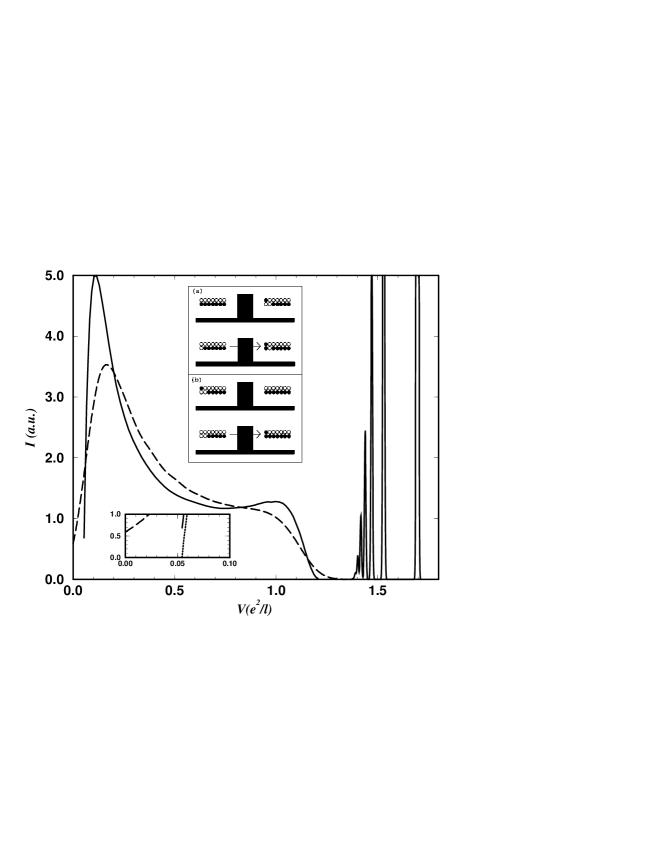
FIG. 1.: Tunneling I-V in the presence of skyrmions for disk (solid line) and spherical (dashed line) geometries (see text.) Upper inset: Schematic representation of the two possible tunneling processes. (a) A majority-spin electron tunnels into a skyrmion. (b) A minority-spin electron tunnels from the skyrmion into a ferromagnetic region. (Only the dominant Slater determinant is shown.) Lower inset: Blow-up of the low voltage region of $I-V$ using simple (solid line) and improved (dotted line) wavefunctions. See text.

REFERENCES

- [1] The Quantum Hall Effect, 2nd Ed., edited by R. E. Prange and S. M. Girvin (Springer, New York, 1990).
- [2] F. P. Milliken, C. P. Umbach, and R. A. Webb, Solid State Comm. 97, 309 (1996); A. M. Chang, L. N. Pfeiffer, and K. W. West, Phys. Rev. Lett. 77, 2538 (1996).
- [3] For a recent review see, C. L. Kane and M. Fisher in Perpectives in Quantum Hall Effects, edited by S. das Sarma and A. Pinczuk (Wiley & Sons, New York, 1997); see also, X. G. Wen, Int. J. Mod. Physics B 6, 1711 (1992).
- [4] J. J. Palacios and A. H. MacDonald, Phys. Rev. Lett. 76, 118 (1996).
- [5] J. P. Einsenstein, L. N. Peiffer, and K. W. West, Phys. Rev. Lett. 69, 3804 (1992); R. C. Ashoori, J. A. Lebens, N. P. Bigelow, and R. H. Silsbee, Phys. Rev. Lett. 64, 681 (1990); ibid., Phys. Rev. B 48, 4616 (1993); H. B. Chan, P. I. Glicofridis, R. C. Ashoori, and M. R. Melloch, preprint, LANL cond-mat/9702088.
- [6] S. He, P. M. Platzman, and B. I. Halperin, Phys. Rev. Lett. 71, 777 (1993); P. Johansson and J. M. Kinaret, Phys. Rev. Lett. 71, 1435 (1993); I. L. Aleiner, H. U. Baranger, and L. I. Glazman, Phys. Rev. Lett. 74, 3435 (1995); R. Haussman, Phys. Rev. B 53, 7357 (1996).
- [7] D.H. Lee and C. L. Kane, Phys. Rev. Lett. 64, 1313 (1990)
- [8] S. L. Sondhi, A. Karlhede, S. A. Kivelson, and E. H. Rezayi, Phys. Rev. B 47, 16419 (1993).
- [9] H. A. Fertig, L. Brey, R. Côté, and A. H. MacDonald, Phys. Rev. B 50 11018 (1994).
- [10] A. H. MacDonald, H. A. Fertig, and L. Brey, Phys. Rev. Lett. 76, 2153 (1996)
- [11] H. A. Fertig, L. Brey, R. Côté, and A. H. MacDonald, Phys. Rev. Lett. 77, 1572 (1996)
- [12] J. J. Palacios, D. Yoshioka, and A. H. MacDonald, Phys. Rev. B 54, R2296 (1996); M. Abolfath, J. J. Palacios, H. Fertig, S. Girvin, and A. H. MacDonald (in preparation).
- [13] J. H. Oaknin, L. Martín-Moreno, and C. Tejedor, Phys. Rev. B 54, 16854 (1996).
- [14] S. E. Barrett, G. Dabbagh, L. N. Pfeiffer, K. W. West, and R. Tycko, Phys. Rev. Lett. 74, 5112 (1995); R. Tycko, S. E. Barrett, G. Dabbagh, L. N. Pfeiffer, and K. W. West, Science 268, 1460 (1995); A. Schmeller, J. P. Eisenstein, L. N. Pfeiffer, and K. W. West, Phys. Rev. Lett. 75, 4290 (1995); E. H. Aifer, B. B. Goldberg, D. A. Broido, Phys. Rev. Lett. 76, 680 (1996).
- [15] D. K. Maude, M. Potemski, J. C. Portal, M. Henini, L. Eaves, G. Hill, and M. A. Pate, Phys. Rev. Lett. 77, 4604 (1996).
- [16] H. A. Fertig, L. Brey, R. Côté, A. H. MacDonald, A. Karlhede, and S. L. Sondhi, to appear in Phys. Rev. B.
- [17] L. Brey, H. A. Fertig, R. Coté, and A. H. MacDonald, Phys. Rev. Lett. 75, 2562 (1995).
- [18] T. Nakajima and H. Aoki, Phys. Rev. Lett. 73, 3568 (1994).
- [19] C. Kallin and B. I. Halperin, Phys. Rev. B 30, 5655 (1984).