Local moment formation in zinc doped cuprates.

Abstract

We suggest that when zinc is substituted for copper in the copper oxide planes of high $T_{c}$ superconductors, it does not necessarily have a valency of $2^{{\scriptscriptstyle+}}$. Rather, the valency of a zinc impurity should be determined by its surrounding medium. In order to study this hypothesis, we examine the effect of static impurities inducing diagonal disorder within a one band Hubbard model coupled to a localised state. We use this model to discuss the physics of zinc doping in the cuprates. Specifically, we discuss the formation of local moments near impurity sites and the modification of the transverse spin susceptibility in the antiferromagnetic state.

I Introduction

The use of a substitutional impurity such as Zn for Cu within the copper oxide planes of the high $T_{c}$ materials[1] is considerably helpful for gaining insight into both the normal and superconducting properties of these systems. Zinc is known to produce a universal rate of $T_{c}$ depression in La,Y,Bi and Tl based high temperature superconductors[2], lending support to a universal pairing mechanism in these cuprates. It is also known to severely affect normal state electronic transport properties, [3, 4] for example inducing semiconducting behaviour in otherwise metallic cuprates.[2, 5] The magnetic behaviour of the high $T_{c}$ oxides is also modified in the presence of zinc. Antiferromagnetic order is destroyed [6, 7] (albeit not as rapidly as superconductivity) and there is a dramatic effect on dynamical spin fluctuations. Whilst the underdoped cuprates are known to possess a spin pseudo gap, Kakurai et.al.[8] have shown that unlike pure ${\rm YBa_{2}Cu_{3}O_{6.6}}$, zinc doped ${\rm YBa_{2}Cu_{2.9}Zn_{0.1}O_{6.6}}$ has no gap like structure in the spin fluctuation spectrum, on the contrary there is a significant enhancement in spectral weight at low frequencies.

It has been suggested that these normal state effects and the observed reduction in $T_{c}$ are related to the formation of local moments observed in the vicinity of the zinc dopants.[9, 10, 11, 12] These moments can be detected by NMR techniques [11, 12, 13, 14] and contribute a Curie law paramagnetism to the magnetic susceptibility.[15, 16] The purpose of this paper is to discuss from a theoretical viewpoint, the formation of such local moments and how they relate to antiferromagnetism and superconductivity.

Recently there has been a considerable amount of interest in local moment formation and its effects on magnetic and superconducting behaviour. Yet there are relatively few theoretical works[17, 18, 19, 20, 21] which attempt to show microscopically how such local moments may form in a two dimensional strongly correlated fermion system. To date, it has been generally believed that zinc substitution results in a Zn⁺⁺ ion situated at a copper site in the superconducting planes. This zinc ion is in a closed $3d^{10}$ configuration and hence the $3d$ holes of the Cu lattice scatter off a static impurity of, from their perspective, very high energy. We wish to suggest here that one cannot assume automatically that the zinc atom is in this valence state. The valency of an atom is effected by its surrounding medium. Accordingly, it is not clear that the role of the zinc $4s$ orbital can be immediately discarded from the conceptual framework, particularly when $3d$ fermions which are experiencing strong Coulomb repulsion are present. In fact, Hao et. al.[22] have shown in an electronic structure calculation of ${\rm La_{1.85}Sr_{0.15}Cu_{1-x}Zn_{x}O_{4}}$, that the partial density of states of the $4s$ orbital is peaked right at the Fermi energy. More ab-initio calculations are required to produce a clearer picture on this point.

In this work we consider local moment formation in a model which reflects the fact that the zinc $3d$ electrons are tightly bound to the nucleus (absence of holes) whilst allowing a coupling between the local $4s$ orbital and the itinerant states of the Cu planar network. To this end our model possesses both Hubbard and Anderson type qualities. We show that, depending on various coupling strengths, local moments are able to form within the Hubbard gap and above and below the Hubbard bands, with spectral weight on and near to the impurity sites. Further, we show that the transverse spin susceptibility at the antiferromagnetic wave vector ${\bf Q}=(\pi,\pi)$ (the lattice spacing is set to unity) indeed gains spectral weight at low frequencies due to the presence of such local moments.

II Theory

Our model Hamiltonian is the following:

$$H=H^{0}+H^{I}+H^{II}\;,$$ (1)

where

$\displaystyle\begin{array}[]{ccl}H^{0}&=&{\displaystyle\sum_{<ij>\sigma}}t(c^{{\scriptscriptstyle{\dagger}}}_{i\sigma}c_{j\sigma}+h.c.)+U{\displaystyle\sum_{i}}c^{{\scriptscriptstyle{\dagger}}}_{i\sigma}c_{i\sigma}c^{{\scriptscriptstyle{\dagger}}}_{i\bar{\sigma}}c_{i\bar{\sigma}}\\ &&\\ &-&{\displaystyle\sum_{i\sigma}}\mu c^{{\scriptscriptstyle{\dagger}}}_{i\sigma}c_{i\sigma}+{\displaystyle\sum_{x\sigma}}(\epsilon^{s}_{x}-\mu)s^{{\scriptscriptstyle{\dagger}}}_{x\sigma}s_{x\sigma}\;,\\ &&\\ H^{I}&=&{\displaystyle\sum_{x\sigma}}\epsilon^{d}_{x}c^{{\scriptscriptstyle{\dagger}}}_{x\sigma}c_{x\sigma}\;,\\ &&\\ H^{II}&=&{\displaystyle\sum_{<xy>\sigma}}t^{\prime}(s^{{\scriptscriptstyle{\dagger}}}_{x\sigma}c_{y\sigma}+h.c.)\;.\end{array}$

The creation operator $c^{{\scriptscriptstyle{\dagger}}}_{i\sigma}$ creates a hole in a $3d$ copper orbital at lattice site $i$ with spin $\sigma$ whilst $c_{j\sigma}$ destroys a $3d$ hole with spin $\sigma$ at lattice site $j$. The first term in $H^{0}$ represents nearest neighbour hopping on a square lattice and the second term is the usual Hubbard interaction between $3d$ holes at the same site. The last term is $H^{0}$ is simply the $4s$ orbital energy level where $\epsilon^{s}_{x}$ is the energy difference between the copper $3d$ and zinc $4s$ hole orbitals. The creation operator $s^{\scriptscriptstyle\dagger}_{x\sigma}$ creates a hole in a zinc $4s$ orbital with spin $\sigma$. The index $x$ labels the impurity sites while $y$ labels an impurity site’s first nearest neighbours. The energy $\epsilon^{d}_{x}$ is the difference between copper and zinc $3d$ hole states. Here $\epsilon^{d}_{x}>0$ whilst $\epsilon^{s}_{x}<0$ and $\mu$ is the chemical potential of the $3d$ system. Thus $H^{I}$ represents static impurity scattering of $3d$ holes off the zinc sites whilst $H^{II}$ reflects a coupling between the localised $4s$ states and the continuum.

In two dimensions the Hubbard model itself has proven to be rather difficult when it comes to theoretical analysis. Consequently, the presence of extra terms in our initial Hamiltonian makes our analytical task no easier. To this end, we employ the finite $U$ slave boson method of Kotliar and Ruckenstein[23] (KR) which, at the mean field level, is in reasonable agreement with Monte Carlo data on the one band 2D Hubbard model[24], and has had similar success with the three band Hubbard model.[25, 26, 27, 28, 29] We use this technique to generate the antiferromagnetic long range order which the 2D Hubbard model is believed to possess at half filling.[30] We are then able to consider the effect of the one body terms $H^{I}$ and $H^{II}$. While our treatment is not self-consistent in the sense the we do not use the effect of $H^{I}$ and $H^{II}$ to recalculate the various bosonic parameters of the KR method, a Hartree Fock self consistent study of a similar model shows that corrections to this approximation are of higher order only.[20]

To generate the antiferromagnetic host we introduce four auxiliary boson fields representing each possible configuration of the $3d$ orbital at a particular site.[23] That is, a $3d$ orbital may be empty, singly occupied with a spin $\sigma$ or doubly occupied. The fermionic creation operator is mapped $c^{{\scriptscriptstyle{\dagger}}}_{i\sigma}\mapsto z_{i\sigma}c^{{\scriptscriptstyle{\dagger}}}_{i\sigma}$, where $z_{i\sigma}$ is defined as

$$z_{i\sigma}\equiv\frac{e_{i}p^{{\scriptscriptstyle{\dagger}}}_{i\sigma}+p_{i\bar{\sigma}}d^{{\scriptscriptstyle{\dagger}}}_{i}}{\sqrt{(1-d^{{\scriptscriptstyle{\dagger}}}_{i}d_{i}-p^{{\scriptscriptstyle{\dagger}}}_{i\sigma}p_{i\sigma})(1-e^{{\scriptscriptstyle{\dagger}}}_{i}e_{i}-p^{{\scriptscriptstyle{\dagger}}}_{i\bar{\sigma}}p_{i\bar{\sigma}})}}\;.$$ (2)

There is a conjugate mapping for the fermionic destruction operator. The boson fields $e_{i},p_{i\sigma}$ and $d_{i}$ represent empty, single with spin $\sigma$ an double occupation of the $3d$ orbital at a site $i$ respectively. The denominator in Eq. (2) ensures that the mapping becomes trivial in the limit $U\rightarrow 0$. Unphysical states arising from the enlargened Hilbert space are eliminated via the following constraints:

$$c^{{\scriptscriptstyle{\dagger}}}_{i\sigma}c_{i\sigma}=p^{{\scriptscriptstyle{\dagger}}}_{i\sigma}p_{i\sigma}+d^{{\scriptscriptstyle{\dagger}}}_{i}d_{i}$$ (3)

and

$$e^{{\scriptscriptstyle{\dagger}}}_{i}e_{i}+\sum_{\sigma}p^{{\scriptscriptstyle{\dagger}}}_{i\sigma}p_{i\sigma}+d^{{\scriptscriptstyle{\dagger}}}_{i}d_{i}=1$$ (4)

which imply charge conservation and completeness of the bosonic operators respectively. Introducing the constraints into the Hamiltonian $H^{0}$ via Lagrange multipliers we have,

$$H^{0} = \sum_{<ij>\sigma}t(q_{\sigma}c^{{\scriptscriptstyle{\dagger}}}_{i\sigma}c_{j\sigma}+h.c.)+U\sum_{i}d^{{\scriptscriptstyle{\dagger}}}_{i}d_{i}$$ (5)

$$+ \sum_{i\sigma}(\lambda_{i\sigma}-\mu)(c^{{\scriptscriptstyle{\dagger}}}_{i\sigma}c_{i\sigma}-p^{{\scriptscriptstyle{\dagger}}}_{i\sigma}p_{i\sigma}+d^{{\scriptscriptstyle{\dagger}}}_{i}d_{i})$$ (6)

$$+ \sum_{i}\lambda^{\prime}_{i}(e^{{\scriptscriptstyle{\dagger}}}_{i}e_{i}+\sum_{\sigma}p^{{\scriptscriptstyle{\dagger}}}_{i\sigma}p_{i\sigma}+d^{{\scriptscriptstyle{\dagger}}}_{i}d_{i}-1)$$ (7)

$$+ {\displaystyle\sum_{x\sigma}}\epsilon^{s}_{x}s^{{\scriptscriptstyle{\dagger}}}_{x\sigma}s_{x\sigma}\;,$$ (8)

where $q_{ij\sigma}=z_{i\sigma}z^{*}_{j\sigma}$.

To accommodate the antiferromagnetic phase of the Hubbard model we split the square lattice into two sub-lattices $A$ and $B$. The symmetry of this phase implies

$\displaystyle n_{{\scriptscriptstyle A}\sigma}=n_{{\scriptscriptstyle B}\bar{\sigma}}\equiv n_{\sigma}\;.$

In terms of the bosons,

$\displaystyle\langle p^{{\scriptscriptstyle{\dagger}}}_{{\scriptscriptstyle A}\sigma}p_{{\scriptscriptstyle A}\sigma}\rangle=\langle p^{{\scriptscriptstyle{\dagger}}}_{{\scriptscriptstyle B}\bar{\sigma}}p_{{\scriptscriptstyle B}\bar{\sigma}}\rangle\equiv\langle p^{{\scriptscriptstyle{\dagger}}}_{\sigma}p_{\sigma}\rangle\;,$

$\displaystyle\langle e^{{\scriptscriptstyle{\dagger}}}_{{\scriptscriptstyle A}}e_{{\scriptscriptstyle A}}\rangle=\langle e^{{\scriptscriptstyle{\dagger}}}_{{\scriptscriptstyle B}}e_{{\scriptscriptstyle B}}\rangle\equiv\langle e^{{\scriptscriptstyle{\dagger}}}e\rangle\;,$

and

$\displaystyle\langle d^{{\scriptscriptstyle{\dagger}}}_{{\scriptscriptstyle A}}d_{{\scriptscriptstyle A}}\rangle=\langle d^{{\scriptscriptstyle{\dagger}}}_{{\scriptscriptstyle B}}d_{{\scriptscriptstyle B}}\rangle\equiv\langle d^{{\scriptscriptstyle{\dagger}}}d\rangle\;.$

We also have $\lambda_{{\scriptscriptstyle A}\sigma}=\lambda_{{\scriptscriptstyle B}\bar{\sigma}}\equiv\lambda_{\sigma}$. The partition function corresponding to $H^{0}$ can be calculated exactly in the fermion sector and at the saddle point in the boson sector (where the bosonic fields become $c$ numbers). The self consistent mean field equations can then be solved. At half filling the chemical potential $\mu=(\lambda_{{\scriptscriptstyle\uparrow}}+\lambda_{{\scriptscriptstyle\downarrow}})/2$.

At the mean field level, the quasiparticle bandstructure is given by

$$E_{{\bf k}\nu\sigma}=\nu\sqrt{\Delta^{2}+q^{2}\epsilon({\bf k})^{2}}$$ (10)

where $\epsilon({\bf k})$ is the 2D square lattice tight binding band structure, $\Delta=(\lambda_{{\scriptscriptstyle\uparrow}}-\lambda_{{\scriptscriptstyle\downarrow}})/2$ and $\nu=\pm$ which refers to the upper and lower Hubbard bands respectively. The quasiparticle amplitudes on each sub-lattice are:

$$a_{{\bf k}\nu\sigma}^{2}=\frac{q^{2}\epsilon({\bf k})^{2}}{q^{2}\epsilon({\bf k})^{2}+(E_{{\bf k}\nu\sigma}-\sigma\Delta)^{2}}\;,$$ (11)

and by symmetry,

$$b_{{\bf k}\nu\bar{\sigma}}^{2}=a_{{\bf k}\nu\sigma}^{2}\;,$$ (12)

where $a_{{\bf k}\nu\sigma}$ refers to the $A$ sub-lattice and $b_{{\bf k}\nu\sigma}$ to the $B$ sub-lattice.

The Green’s function of $H^{0}$ may be written as,

$${\rm{\bf G}}^{0}_{\sigma}({\bf k},\omega)=\left[\begin{array}[]{ll}{\rm G}^{0c}_{\sigma}({\bf k},\omega)&\\ &\\ &{\rm G}^{0s}_{\sigma}(\omega)\\ \end{array}\right]\;,$$ (13)

where ${\rm G}^{0c}_{\sigma}({\bf k},\omega)$ is the Green’s function for the continuum states and is itself a ${\rm 2x2}$ matrix because of the sub-lattice structure. The Green’s function ${\rm G}^{0s}_{\sigma}(\omega)$ is due to the localised $4s$ state. Specifically, they are;

$${\rm G}^{0c}_{\sigma}({\bf k},\omega)=\sum_{\nu}\left[\begin{array}[]{cc}a_{{\bf k}\nu\sigma}^{2}&a_{{\bf k}\nu\sigma}^{*}b_{{\bf k}\nu\sigma}\\ &\\ a_{{\bf k}\nu\sigma}b_{{\bf k}\nu\sigma}^{*}&b_{{\bf k}\nu\sigma}^{2}\\ \end{array}\right]\frac{1}{\omega-E_{{\bf k}\nu\sigma}\pm i\eta}$$ (14)

and

$${\rm G}^{0s}_{\sigma}(\omega)=\frac{1}{\omega-(\epsilon^{s}_{x}-\mu)}$$ (15)

where $\pm i\eta$ refers to the upper and lower Hubbard bands respectively.

We initially consider the effect of one zinc impurity positioned on the $A$ sub-lattice. Formally it is simpler to first take into account the effect of $H^{I}$. The $T$- matrix expression for the continuum Green’s function in real space is:

$${\rm G}^{Ic}_{ij\sigma}(\omega)={\rm G}^{0c}_{ij\sigma}(\omega)+\frac{{\rm G}^{0c}_{ix\sigma}(\omega)\epsilon^{d}_{x}{\rm G}^{0c}_{xj\sigma}(\omega)}{1-\epsilon^{d}_{x}{\rm G}^{0c}_{xx\sigma}(\omega)}\;,$$ (16)

and of course ${\rm G}^{Is}_{\sigma}(\omega)={\rm G}^{0s}_{\sigma}(\omega)$.

Including now the scattering contributions of $H^{II}$, the full continuum Green’s function of $H$ in real space is:

$${\rm G}^{c}_{ij\sigma}(\omega)={\rm G}^{Ic}_{ij\sigma}(\omega)+\frac{{\textstyle\sum_{yy^{\prime}}}{\rm G}^{Ic}_{iy}(\omega)t^{\prime}{\rm G}^{Is}_{\sigma}(\omega)t^{\prime}{\rm G}^{Ic}_{y^{\prime}j\sigma}(\omega)}{1-t^{\prime}{\rm G}^{Is}_{\sigma}(\omega)t^{\prime}{\textstyle\sum_{yy^{\prime}}}{\rm G}^{Ic}_{yy^{\prime}\sigma}(\omega)}\;,$$ (17)

and the full local state Green’s function can be written as

$${\rm G}^{s}_{\sigma}(\omega)=\frac{1}{w-(\epsilon^{s}_{x}-\mu)-\Sigma(\omega)}\;,$$ (18)

where $\Sigma(\omega)$ is a self energy given by $\Sigma(\omega)={\textstyle\sum_{yy^{\prime}}}t^{\prime}{\rm G}^{Ic}_{yy^{\prime}}(\omega)t^{\prime}$.

The poles of ${\rm G}^{c}_{ij\sigma}(\omega)$ and ${\rm G}^{s}_{\sigma}(\omega)$ give the discrete states of the system. They are given by the solution of

$$\begin{array}[]{ll}\left(\omega-(\epsilon^{s}_{x}-\mu)\right)\left(1-\epsilon^{d}_{x}{\rm G}^{0c}_{xx\sigma}(\omega)\right)-{\displaystyle\sum_{yy^{\prime}}}{t^{\prime}}^{2}\epsilon^{d}_{x}{\rm G}^{0c}_{yy^{\prime}\sigma}(\omega)&\\ -{\displaystyle\sum_{yy^{\prime}}}{t^{\prime}}^{2}\left(1-\epsilon^{d}_{x}{\rm G}^{0c}_{xx\sigma}(\omega)\right){\rm G}^{0c}_{xy\sigma}(\omega){\rm G}^{0c}_{y^{\prime}x\sigma}(\omega)=0\;.&\\ \end{array}$$ (19)

Note that in the limit $t^{\prime}\rightarrow 0,\epsilon^{d}_{x}\rightarrow 0$ we recover the discrete $4s$ state.

To determine if the discrete states (which are the solutions of Eq.(19)) are localised in nature we can calculate the probability of finding a particle with spin $\sigma$ occupying one of these states at the impurity site or at its nearest neighbours through the residues of the appropriate Green’s functions. For example, for the $4s$ state we use Res$[{\rm G}^{s}_{\sigma}(\omega);\omega=E_{dis}]$, for the $3d$ state at the $x$ site we have Res$[{\rm G}^{c}_{xx\sigma}(\omega);\omega=E_{dis}]$ and for the nearest neighbour $3d$ states we use Res$[{\rm G}^{c}_{xy\sigma}(\omega);\omega=E_{dis}]$. Here $E_{dis}$ is the energy of the discrete state in question.

III Results

A Local moments

We have used in our calculations a value of $U=6.4t$ which produces a gap of $2\Delta=4t$ and a chemical potential for the half filled $3d$ antiferromagnetic system of $\mu=-3.49t$. We have also set the impurity $3d$ orbital energy at $\epsilon^{d}_{x}=9t$. This enables us to explore as a function of $\epsilon^{s}_{x}-\mu$ and $t^{\prime}$ the nature of the discrete states which form in the whole system.

It is appropriate to first discuss the energy structure of the various orbital energy levels and quasiparticle bands. In Fig.1 we show this relationship. The copper $3d$ hole orbital energy is used as a reference. The two quasiparticle bands are shown as well as where the Fermi level sits and the quantity $\epsilon^{s}_{x}-\mu$. Thus when $\epsilon^{s}_{x}-\mu=0$ one is considering a zinc $4s$ hole level roughly $3.49t$ below the copper $3d$ hole level. A large value of $|\epsilon^{s}_{x}-\mu|$ would be favourable for zinc to acquire a valency of $2^{{\scriptscriptstyle+}}$ as the $4s$ discrete state would become occupied by holes.

Solutions to Eq.(19) for $\epsilon^{d}_{x}>0$ and for any values of $\epsilon^{s}_{x}-\mu$ and $t^{\prime}$ produce two discrete states above the upper Hubbard band (in the hole picture). With increasing $\epsilon^{d}_{x}$ they become completely localised to the impurity $3d$ orbital. Accordingly they represent localised zinc $3d$ electrons. The appearance of gap states or states below the lower band depends on the combination of the above parameters.

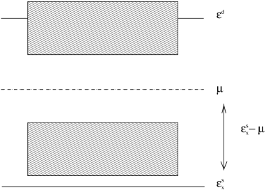
FIG. 1.: Energy structure of the hole orbital energies and bands (shaded regions).

Without any coupling to the $4s$ state the system produces one gap state [19] which has a reasonable amount of spectral weight on its nearest neighbours, producing a local moment. In the limit $\epsilon^{d}_{x}\rightarrow\infty$ the spectral weight of the gap state is completely removed from the impurity site. In general, for fixed $\epsilon^{d}_{x}=9t$, a coupling to the $4s$ state produces one or two extra gap states depending on $t^{\prime}$ and $\epsilon^{s}_{x}-\mu$. These are the remnants of the $4s$ localised states however some of their spectral weight has been shifted to the nearest neighbours by differing amounts depending on spin, which in effect produces a local moment occupying the $4s$ state. In Fig.2 we give an example of the graphical form of Eq.(19) for a parameter set of $t^{\prime}=0.25t$ and $\epsilon^{s}_{x}-\mu=-2t$.

FIG. 2.: The intersections with the horizontal axis give the discrete states of the system. Here we show an example for $t^{\prime}=0.25t,\epsilon^{s}_{x}-\mu=-2t$ and $\epsilon^{d}_{x}=9t$.The region between the first two dotted vertical lines is the lower band and the region between the second pair is the upper band.

We can see by the intersections with the horizontal axis in Fig.2, that two gap states have formed as have two states above the hole upper band. These last two states are strongly localised in the zinc $3d$ orbital and show that this orbital is filled with electrons. The up spin gap state has amplitude mainly on the zinc neighbours however the down spin gap state has amplitude mainly in the zinc $4s$ orbital. Thus we have two local moment contributions. One situated at the zinc site and one spread mainly over the nearest neighbours. Both spins are in opposite alignment to the antiferromagnetically aligned moments of their respective sub-lattices.

Both localised gap states are able to act as unpaired moments which should contribute a Curie like behaviour to the temperature dependent susceptibility. With more impurity doping and therefore more localised states, the antiferromagnetic correlation length will be reduced leading to an eventual loss of antiferromagnetic order. Calculations by Sen et al.[19] have shown that in the presence of local moments, the spin-wave stiffness vanishes beyond a certain length scale, destroying long range antiferromagnetic order.

FIG. 3.: Local moment $m=n_{\uparrow}-n_{\downarrow}$ as a function of $(\epsilon^{s}_{x}-\mu)/t$ for the $4s$ orbital, the $3d$ orbital at the zinc site$(3d_{x})$ and the $3d$ orbital of one of the nearest neighbours$(3d_{y})$.

For $t^{\prime}=0.25t,$ if $\epsilon^{s}_{x}-\mu$ is situated in the gap then an up spin gap state and a down spin gap state form with large amplitudes in the $4s$ orbital and thus there is no local moment contribution from the $4s$ states. Accordingly the zinc atom is nearly inert. An additional up spin gap state forms with amplitude mainly on the neighbouring sites producing a local moment. If however $\epsilon^{s}_{x}-\mu$ is situated within a small energy window between $-3t$ and $-1.5t$, then the up spin gap state with amplitude mainly on the $4s$ orbital is lost, leaving only the down spin state which in effect leads to a local moment at the zinc site. There is still a local moment from the remaining up spin gap state whose amplitude is found mainly on neighbouring sites. If $\epsilon^{s}_{x}-\mu$ is too negative then hole bound states are formed below the bands in the $4s$ orbitals. In Fig.3 we show the net moment produced by the discrete states as a function of $\epsilon^{s}_{x}-\mu$ in units of $t$ for $t^{\prime}=0.25t$.

It can be seen that the valence of a zinc impurity cannot be simply assumed to be $2^{{\scriptscriptstyle+}}$. Our purpose here has been to show that the valence of a zinc atom can only be considered in the presence of strongly correlated $3d$ fermions.

B Spin Fluctuations

It is instructive to examine the effect of localised states on spin fluctuation excitations. Attempts at calculating the spin fluctuation spectrum of an itinerant antiferromagnet such as the 2D Hubbard model have generally involved a mean field plus RPA type approach[31] which attempts to incorporate Gaussian fluctuations around the antiferromagnetic saddle point. This avenue of attack has been successful in producing low frequency spin wave modes in the large $U$ limit with dispersion which agrees with linear spin wave theory of the 2D Heisenberg antiferromagnet.[32] Here, we do not attempt to calculate a renormalised susceptibility by including fluctuations, but instead we calculate the modification of the bare susceptibility of the antiferromagnetic mean field state due to the presence of local moments in an attempt to illustrate that the presence of local moments causes an increase in spectral weight in the spin fluctuation spectrum, particularly at low frequencies.

Even at this level the full calculation is in general quite complicated. Thus, as an example we calculate the contributions from localised states produced purely by the impurity energy $\epsilon^{d}_{x}$. Thus we set $t^{\prime}=0$ and so ignore any contributions from localised states formed by coupling of the conduction holes to the localised $4s$ state.

The transverse spin fluctuations of the rigid antiferromagnetic host can be described by a 2x2 matrix

$${\bf\chi}^{0c}({\bf Q},\omega)=\left[\begin{array}[]{ll}\chi_{aa}^{0c}({\bf Q},\omega)&\chi^{0c}_{ab}({\bf Q},\omega)\\ &\\ \chi^{0c}_{ba}({\bf Q},\omega)&\chi^{0c}_{bb}({\bf Q},\omega)\end{array}\right]\;,$$ (20)

where $a$ and $b$ label the sub-lattices and the elements of $\chi^{0c}({\bf Q},\omega)$ are defined as

$$\begin{array}[]{l}\chi^{0c}_{mn}({\bf Q},\omega)=\\ \\ {\displaystyle\frac{i}{2\pi N}\sum_{{\bf p}}\int^{\infty}_{-\infty}dE^{\prime}{\rm G}^{0c}_{mn{\scriptscriptstyle\uparrow}}}({\bf p},E^{\prime}){\rm G}^{0c}_{nm{\scriptscriptstyle\downarrow}}({\bf p}-{\bf Q},E^{\prime}-\omega)\;,\\ \end{array}$$ (21)

where $m$ and $n$ are either $a$ or $b$. The full spin susceptibility matrix elements are similarly defined. That is, we have

$$\begin{array}[]{l}{\bf\chi}^{c}_{mn}({\bf Q},\omega)=\\ \\ {\displaystyle\frac{i}{2\pi N}\sum_{{\bf p}}\int^{\infty}_{-\infty}dE^{\prime}{\rm G}^{Ic}_{mn{\scriptscriptstyle\uparrow}}}({\bf p},E^{\prime}){\rm G}^{Ic}_{nm{\scriptscriptstyle\downarrow}}({\bf p}-{\bf Q},E^{\prime}-\omega)\;.\\ \end{array}$$ (22)

For simplicity we assume a small concentration of impurities distributed evenly over the two sub-lattices such that multiple scattering from different sites may be safely neglected. The diagonal continuum Green’s functions can be written in momentum space as

$${\rm G}^{c}_{mm\sigma}({\bf k},\omega) = {\rm G}^{0c}_{mm\sigma}({\bf k},\omega)+\frac{\epsilon^{d}_{x}n_{x_{m}}}{1-\epsilon^{d}_{x}{\rm G}^{0c}_{x_{m}x_{m}\sigma}}{\rm G}^{0c}_{mm}({\bf k},\omega)^{2}$$ (23)

$$+ \frac{\epsilon^{d}_{x}n_{x_{\bar{m}}}}{1-\epsilon^{d}_{x}{\rm G}^{0c}_{x_{\bar{m}}x_{\bar{m}}\sigma}}{\rm G}^{0c}_{m\bar{m}\sigma}({\bf k},\omega){\rm G}^{0c}_{\bar{m}m\sigma}({\bf k},\omega)\;,$$ (24)

where $n_{x_{m}}$ is the concentration of impurities on the $m$ sub-lattice. The diagonal components of the susceptibility can be calculated by carrying out contour integrations in the upper and lower halves of the complex plane, making sure to take into account the poles on the real axis due to the discrete states.

In Fig.4 we have evaluated at ${\bf Q}=(\pi,\pi)$ the imaginary part of the localised state contributions to the diagonal components of ${\bf\chi}^{c}({\bf Q},\omega)$ up to first order in impurity concentration of $n_{x_{a}}=n_{x_{b}}=0.05$ (full curve). We have calculated the contributions to the spectral weight of spin fluctuations by scattering processes within the bands and they are negligible. The dashed curves are the sum of the imaginary parts of the diagonal components of $\chi^{0c}({\bf Q},\omega)$. At this level they represent particle-hole excitations only. We have set $\epsilon^{d}_{x}=5t$ which produces for each impurity one gap state and two states above the upper Hubbard band in the hole picture. It can be seen that the contribution from these localised states is an enhancement in the spectral weight at low frequencies.

The increase in spectral weight at low frequencies would be further enhanced if one were to include the off diagonal processes which contribute to $\chi^{c}({\bf Q},\omega)$ (which are due to inter sub lattice excitations), as well as the contribution from any extra localised states produced by a coupling of the itinerant states to the zinc $4s$ states via $t^{\prime}$.

FIG. 4.: Imaginary part of the transverse spin susceptibility at ${\bf Q}=(\pi,\pi)$. Here $\epsilon^{d}_{x}=5t$. The dashed line is the sum of the diagonal components of Im $\chi^{0c}({\bf Q},\omega)$ whilst the solid line represents the contributions from the discrete states.

Indeed if this increase in spectral weight is also produced away from half filling then this phenomena may go some way in explaining how the spin pseudo gap in the underdoped compounds vanishes with zinc doping. As Tallon et al.[33] have pointed out, for a small amount of zinc doping the pseudo gap is suppressed near the vicinity of the dopants and may be completely suppressed when the mean spacing between zinc atoms falls below the pseudo gap correlation length.

In this picture superconductivity would also be extinguished when the pair correlation length falls below the mean spacing between zinc atoms. Pair breaking could occur via the Abrikosov-Gorkov mechanism due to effective magnetic scattering, however there is evidence to suggest that this effect is too small to account for the rapid reduction of $T_{c}$.[13] If the order parameter has $d_{x^{2}-y^{2}}$ symmetry then in addition to the this, strong potential scattering from the zinc impurities may be enough to suppress $T_{c}$ at a rate seen by experiment.

Alternatively, if in the underdoped materials, the formation of a spin pseudo gap is related to the formation of local singlet pairs, then suppression of this gap due to an increase in spin excitation spectral weight may also be a possible explanation for the reduction of $T_{c}$.

IV Conclusions

We have attempted to show that when substituting zinc for copper within the copper oxide planes one cannot assume that zinc is in the $2^{{\scriptscriptstyle+}}$ state. Rather , its valency is sensitive to the presence of a strongly correlated system. We have shown that local moment formation is possible on and near the zinc sites and that they produce an enhancement of the low energy spectral weight of antiferromagnetic spin fluctuations.

V Acknowledgements

We would like to thank T.C. Choy and M. Gulacsi for useful discussions. B.C.dH would like to thank the Commonwealth Government of Australia for providing financial assistance.

REFERENCES

- [1] Gang Xiao, M.Z. Cieplak, A. Gavrin, F.H. Streitz, A. Bakhshai and C.L. Chien, Phys. Rev. Lett. 60, 1446 (1988).
- [2] S.K. Agarwal and A.V. Narlikar, Prog. Crystal Growth and Charact. 28, 219 (1994).
- [3] S. Zagoulaev, P. Monod and J.Jégoudez, Phys. Rev. B 52, 10474 (1995).
- [4] S. Uchida, Y Fukuzumi, K. Mizuhashi and K. Takenaka, Chinese J. Phys. 34, 423 (1996).
- [5] V.P.S Awana, S.K. Agarwal, M.P. Das and A.V. Narlikar, J. Phys.: Condens. Matter 4 4971 (1992).
- [6] Gang Xiao, Marta Z. Cieplak and C.L. Chien, Phys Rev B 42, 240 (1990).
- [7] B. Keimer, A. Aharony, A. Auerbach, R.J. Birgeneau, A. Cassanho, Y. Endoh, R.W. Erwin, M.A. Kastner and G. Shirane, Phys. Rev. B 45, 7430 (1992).
- [8] K. Kakurai, S. Shamoto, T. Kiyokura, M. Sato, J.M. Tranquada and G. Shirane, Phys. Rev. B 48, 3485 (1993).
- [9] G.V.M. Williams, J.L. Tallon and R. Meinhold, Phys. Rev. B 52, 7034 (1995).
- [10] J.R. Cooper and J.W. Loram, preprint(1996).
- [11] H. Alloul, P.Mendels, H. Casalta, J.F. Marucco and J. Arabski, Phys. Rev. Lett. 67, 3140 (1991).
- [12] A.V. Mahajan, H.Alloul, G.Collin and J.F. Marucco, Phys. Rev. Lett. 72, 3100 (1994).
- [13] R.E. Walstedt, R.F. Bell, L.F. Schneemeyer, J.V. Waszczak, W.W. Warren Jr., R. Dupree and A. Gencten, Phys. Rev. B 48, 10646 (1993).
- [14] Kenji Ishida, Yoshio Kitaoka, Nobuhito Ogata, Takeshi Kamino, Kunisuke Asayama, J.R. Cooper and N. Athanassopoulou, J. Phys. Soc. Jpn. 62, 2803 (1993).
- [15] Chan-Soo Jee, D. Nichols, A.Kebede, S. Rahman, J.E. Crow, A.M. Ponte Goncalves, T. Mihalisin, G.H. Myer, I. Perez, R.E. Salomon, P. Schlottmann, S.H. Bloom, M.V. Kuric amd Y.S. Yao, J. Supercond. 1, 63 (1988).
- [16] S. Zagoulaev, P. Monod and J.Jégoudez, Physica C 259, 271 (1996).
- [17] W. Zeigler, D. Poiblanc, R. Preuss, W. Hanke and D.J. Scalapino, Phys. Rev. B 53, 8704 (1996).
- [18] Prasenjit Sen, Saurabh Basu and Avinash Singh, Phys. Rev. B 50, 10382 (1994).
- [19] Prasenjit Sen and Avinash Singh, Phys. Rev. B 53, 328 (1996).
- [20] Saurabh Basu and Avinash Singh, Phys. Rev. B 53, 6406 (1996).
- [21] S.G. Ovchinnikov, Phys. Solid State 37, 2007 (1995).
- [22] Hao Xue-Jun, Zhou Yun-Song and Zhang Li-Yuan, Mod. Phys. Lett. B 8, 641 (1994).
- [23] G. Kotliar and A.E. Ruckenstein, Phys. Rev. Lett. 57, 1362 (1986).
- [24] L. Lilly, A. Maramatsu and W. Hanke, Phys. Rev. Lett. 65, 1379 (1990).
- [25] V.J. Emery, Phys. Rev. Lett. 58, 2794 (1987).
- [26] P.B. Littlewood, C.M. Varma and E. Abrahams, Phys. Rev. Lett. 60, 379 (1987).
- [27] B.C. den Hertog and M.P. Das, Phys. Rev. B 54, 6693 (1996).
- [28] B.C. den Hertog and M.P. Das, Solid State Commun. 98, 7 (1996).
- [29] Weiyi Zhang, M. Avignon and K.H. Bennemann, Phys. Rev. B 42, 10192 (1990).
- [30] J.E. Hirsch and S. Tang, Phys. Rev. Lett. 62, 591 (1989).
- [31] J.R. Schrieffer, X.G. Wen and S.C. Zhang, Phys. Rev. B 39, 11663 (1989).
- [32] A.P. Kampf, Phys. Rep. 249, 219 (1994).
- [33] J.L. Tallon, J.R. Cooper, P.S.I.P.N. de Silva, G.V.M. Williams and J.W. Loram, Phys. Rev. Lett. 75, 4114 (1995).