[

Phase diagram of the one-dimensional Holstein model of spinless fermions

Abstract

The one-dimensional Holstein model of spinless fermions interacting with dispersionless phonons is studied using a new variant of the density matrix renormalization group. By examining various low-energy excitations of finite chains, the metal-insulator phase boundary is determined precisely and agrees with the predictions of strong coupling theory in the anti-adiabatic regime and is consistent with renormalization group arguments in the adiabatic regime. The Luttinger liquid parameters, determined by finite-size scaling, are consistent with a Kosterlitz-Thouless transition.

]

The challenge of understanding superconductivity in fullerenes, bismuth oxides, and the high-$T_{\text{c}}$ cuprates has renewed interest in models of interacting electrons and phonons [2]. Unlike conventional metals these materials are not necessarily in the weak-coupling regime where perturbation theory can be used or the strong-coupling regime in which a polaronic treatment is possible [2]. Neither are they necessarily in the adiabatic regime in which characteristic phonon energies are much less than characteristic electronic energies. This challenge has led to numerical studies of the Holstein (or molecular crystal) model of electrons interacting with dispersionless phonons in infinite dimensions, two dimensions, one dimension and on just two sites (see the references in [2, 3]). The one-dimensional case is important because of the wide range of quasi-one-dimensional materials which undergo a Peierls or charge-density-wave (CDW) instability due to the electron-phonon interaction. Most theoretical treatments assume the adiabatic limit and treat the phonons in a mean-field approximation. However, it has been argued that in many CDW materials the quantum lattice fluctuations are important [4].

In this Letter we present a study of the one-dimensional Holstein model of spinless fermions at half-filling using the density matrix renormalization group (DMRG). This model is particularly interesting because at a finite fermion-phonon coupling there is a quantum phase transition from a Luttinger liquid (metallic) phase to an insulating phase with CDW long-range order [5, 6]. This illustrates how quantum fluctuations can destroy the Peierls state. The Hamiltonian is

$${\cal H} = -t\sum_{i=1}^{N}\left(c_{i}^{\dagger}c_{i+1}+c_{i+1}^{\dagger}c_{i}\right)+\omega\sum_{i=1}^{N}a_{i}^{\dagger}a_{i}$$ (2)

$$-\;g\sum_{i=1}^{N}\left(c_{i}^{\dagger}c_{i}-\frac{1}{2}\right)\left(a_{i}+a_{i}^{\dagger}\right),$$

where $c_{i}$ destroys a fermion on site $i$, $a_{i}$ destroys a local phonon of frequency $\omega$, $t$ is the hopping integral, $g$ is the fermion-phonon coupling and a periodic chain of $N$ sites is assumed. The phase transition occurs at a critical coupling $g_{\text{c}}$ separating metallic ($0\leq g\leq g_{\text{c}}$) and CDW insulating phases ($g>g_{\text{c}}$) [5, 6]. In the strong coupling limit ($g^{2}>>\omega t$) (2) can be mapped onto the anisotropic, antiferromagnetic Heisenberg ($XXZ$) model [5] which is exactly soluble. The transition occurs at the spin isotropy point, is of the Kosterlitz-Thouless (K-T) type, and the Luttinger liquid parameters can be found in the metallic phase [3].

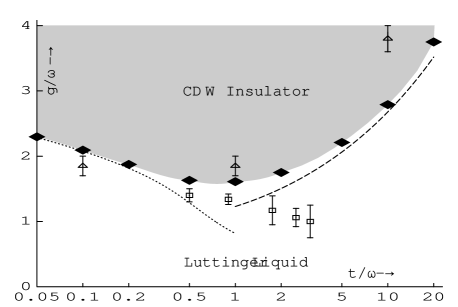
FIG. 1.: Zero temperature phase diagram of the one-dimensional Holstein model of spinless fermions at half-filling. For small fermionic-phonon coupling $g$ the system is a Luttinger liquid with parameters that vary with the coupling. For large $g$ the system has an energy gap and long-range charge-density-wave (CDW) order. The solid diamonds denote the phase boundary from this DMRG study. The systematic errors are smaller than the diamonds. The results of previous quantum Monte Carlo studies are denoted by squares [5] and triangles [3]. The dotted line is the phase boundary from strong coupling theory [5] and the dashed line is defined by $\omega=\Delta_{\text{MF}}$ (where $\Delta_{\text{MF}}\equiv 8te^{-\pi t\omega/g^{2}}$ is the mean-field energy gap) and is the approximate location of the phase boundary predicted by a two-cutoff renormalization group scheme [16].

The phase diagram of (2) over a wide range of adiabacity parameters ($0.05\leq t/\omega\leq 20$) is shown in Fig. 1. A new variant [7] of the DMRG method [8, 9, 10, 11] is used to determine the energy of low-lying excitations to a far greater precision than previous quantum Monte Carlo (QMC) studies [3, 5]. Finite-size scaling (FSS) of a number of energy gaps permits the accurate determination of $g_{\text{c}}$ and the Luttinger liquid parameters.

The study of fermion-boson models such as (2) by exact diagonalization or the DMRG presents a challenge because there are an infinite number of phonon quantum states on each site. Caron and Moukouri have studied the $XY$ spin-Peierls and free acoustic phonons models [9] on open chains using a conventional DMRG algorithm. The simple truncation of the phonon Hilbert space used in these calculations can require an excessively large number of states, to the extent where the effort expended in representing a single site becomes comparable to that expended in representing a block. This becomes important when trying to study periodic systems (which are more useful for FSS studies) where an extra site is usually added to avoid direct interactions between blocks. Jeckelmann and White devised a scheme that maps bosons onto fermions which they applied to the polaron problem (a single electron interacting with the phonons) in one and two dimensions [10]. A more promising method, which dramatically reduces the number of states required to represent a site, has been used to examine small (6 site), half-filled Holstein systems using exact diagonalization [11]. We have developed a somewhat similar DMRG algorithm which is designed to solve periodic systems with a large number of degrees of freedom per site. The details of the method will be published elsewhere [7]—here we concentrate on the results for (2).

The good quantum numbers used are the total fermion number $\hat{N}\equiv\sum_{i=1}^{N}c_{i}^{\dagger}c_{i}$, and, for the neutral case ($\frac{1}{2}$-filled band; $\hat{N}=N/2$), the parity (particle-hole) operator $\hat{P}:c_{i}\mapsto(-1)^{i}c_{i}^{\dagger};a_{i}\mapsto-a_{i}$ The energies calculated are the ground state energy $E_{\text{G}}\equiv E_{0}(\hat{N}=N/2,\hat{P}=1)$, the charge gap $\Delta_{\text{ch}}\equiv E_{0}(\hat{N}=N/2\pm 1)-E_{\text{G}}$, and the 1- and 2- photon gaps (the two lowest neutral excitations [12]) $\Delta_{1}\equiv E_{0}(\hat{N}=N/2,\hat{P}=-1)-E_{\text{G}}$ and $\Delta_{2}\equiv E_{1}(\hat{N}=N/2,\hat{P}=1)-E_{\text{G}}$. A number of accuracy checks were performed: The DMRG reproduces exact results in the non-interacting and strong coupling limits, and the DMRG results agree with QMC results for systems of up to $N=16$ sites [3] within error bars. The DMRG accuracy is determined by the parameter $m$—the number of density matrix eigenstates retained per block. Table I lists convergence results for $\Delta_{\text{ch}}$, along with the QMC results [3]. The DMRG errors, being systematic rather than statistical, are two to three orders of magnitude smaller than the QMC errors.

TABLE I.: Convergence of the charge gap $\Delta_{\text{ch}}$ with the DMRG truncation parameter $m$ for various system sizes $N$ using parameters $t=\omega$ and $g=1.5\omega$. QMC results [3] are included for comparison.

$m$	$N=4$	$N=8$	$N=16$	$N=32$
26	0.4110	0.1971	0.1021	0.05504
36	0.4110	0.1971	0.1004	0.05244
48	0.4110	0.1971	0.1002	0.05148
66	0.4110	0.1971	0.1002	0.05117
78	0.4110	0.1971	0.1001	0.05103
94	0.4110	0.1971	0.1001	0.05099
QMC	0.416(4)	0.200(9)	0.06(3)	–

Typical FSS plots of the various energy gaps are shown in Fig. 2 for the metallic $(g<g_{\text{c}})$ and insulating $(g>g_{\text{c}})$ phases. In the metallic phase the gaps vanish linearly with $1/N$ as $N\rightarrow\infty$, with $\Delta_{1}$ lying above $\Delta_{\text{ch}}$ for large $N$. In the insulating phase $\Delta_{1}$ lies below $\Delta_{\text{ch}}$ and $\Delta_{\text{ch}}$ and $\Delta_{2}$ approach non-zero values as $N\rightarrow\infty$ whilst $\Delta_{1}$ rapidly tends to zero, the state $E_{0}(\hat{N}=N/2,\hat{P}=-1)$ being asymptotically degenerate with the ground state in this phase.

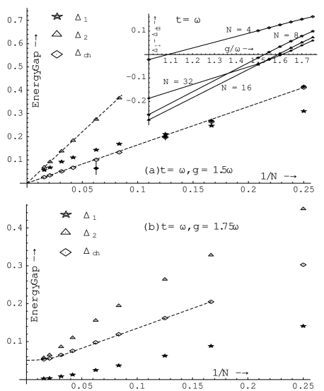
FIG. 2.: Finite-size scaling of the different energy gaps in the (a) Luttinger liquid and (b) insulating phases. The charge gap ($\Delta_{\text{ch}}$) and one- and two- photon gaps ($\Delta_{1}$ and $\Delta_{2}$) are plotted as functions of the inverse lattice size $1/N$ for $t=\omega$ and (a) $g=1.5\omega$ and (b) $g=1.75\omega$. Also shown in case (a) is $\Delta_{\text{ch}}$ as calculated using QMC [3] (solid diamonds with error bars). In (a) the dashed lines are straight lines through the origin, the slope of which can be used to extract the Luttinger liquid exponent $K_{\rho}$ (see Fig. 3). In (b) the dashed line is a guide for the eye. The differences between the two phases are seen in: (i) The relative size of $\Delta_{\text{ch}}$ and $\Delta_{1}$ is opposite for the two phases. (ii) In the limit $N\rightarrow\infty$ the gaps extrapolate to zero (a non-zero value) in the Luttinger liquid (insulating) phase. The inset to (a) shows the difference $\Delta_{1}-\Delta_{\text{ch}}$ as a function of the coupling for various $N$. The critical coupling $g_{\text{c}}$ is determined as the value at which this difference vanishes in the limit $N\rightarrow\infty$.

In the QMC studies [3, 5] the critical point $g_{\text{c}}$ was determined as the point at which an order parameter or the charge gap $\Delta_{\text{ch}}$ becomes non-zero. However, in a K-T transition these quantities behave as $\Delta_{\text{ch}}\sim e^{-A(g-g_{\text{c}})^{-1}}$, and there are nonlinear corrections to FSS which make the precise determination of $g_{\text{c}}$ very difficult by this method. Our method of determining $g_{\text{c}}$ is inspired by work on the frustrated Heisenberg model [13] where the transition point was determined by the crossover of singlet and triplet gaps. It is known that K-T transitions have a hidden $SU(2)$ symmetry [14]. We hypothesise that at $g=g_{\text{c}}$, the states $E_{0}(\hat{N}=N/2\pm 1)$ and $E_{0}(\hat{N}=N/2,\hat{P}=-1)$ form a degenerate triplet in the thermodynamic limit. Plots of the difference $\Delta_{1}-\Delta_{\text{ch}}$ are included in the inset of Fig. 2 for various $N$. A crossover point $g_{\text{c}}(N)$ is defined as the $g$ value at which $\Delta_{1}=\Delta_{\text{ch}}$. $g_{\text{c}}(N)$, listed in Table II for various values of $t/\omega$, approaches $g_{\text{c}}$ as $N\rightarrow\infty$ [15]. The combined errors (DMRG truncation, discretization and fitting in $g$, and extrapolation to $N=\infty$) are estimated to be less than five precent.

TABLE II.: Convergence of the crossover point $g_{\text{c}}(N)/\omega$, determined by $\Delta_{\text{ch}}=\Delta_{1}$, with the system size $N$ for various hopping parameters $t$.

$N$	4	8	16	32	64	128	256
$t=0.1\omega$	2.0878	2.0911	2.0920
$t=\omega$	1.087	1.528	1.591	1.608	1.613
$t=10\omega$				2.220	2.649	2.765	2.788

The resulting phase boundary is shown in Fig. 1, along with the two QMC calculations [3, 5], and the result of strong coupling theory [5] which becomes exact as $t\rightarrow 0$. The DMRG results agree well with the strong coupling curve for $t/\omega<0.2$. For large $t$ the results lie close to the curve defined by $\omega=\Delta_{\text{MF}}\equiv 8te^{-\pi t\omega/g^{2}}$. This curve was predicted to be the approximate phase boundary for $t>\omega$ within a two-cutoff renormalization scheme, where $\Delta_{\text{MF}}$ is the mean-field energy gap [16]. A saddle-point expansion about the mean-field solution [17] suggests that there is a first-order transition for $\omega\sim\Delta_{\text{MF}}$.

We next investigate the nature of the transition and the Luttinger liquid parameters in the metallic phase $(0\leq g\leq g_{\text{c}})$. For a Luttinger liquid of spinless fermions, $E_{\text{G}}$ scales according to $\frac{E_{\text{G}}}{N}\sim\epsilon_{\infty}-\frac{\pi u_{\rho}}{6N^{2}}$ [18], where $\epsilon_{\infty}$ is the bulk ground state energy density and $u_{\rho}$ is the charge velocity. From conformal field theory [19] the scaling forms for the gaps are: $\Delta_{\text{ch}}\sim\frac{\pi u_{\rho}}{2K_{\rho}N}$ and $\Delta_{1},\Delta_{2}\sim\frac{2\pi u_{\rho}K_{\rho}}{N}$, where $K_{\rho}$ is the correlation exponent. The crossover method of determining $g_{\text{c}}$ is equivalent to the assumption that $K_{\rho}=\frac{1}{2}$ at $g=g_{\text{c}}$, i.e., the transition is of the K-T type [20]. In Fig. 3 $u_{\rho}$ (determined from the FSS of $E_{\text{G}}$) and $K_{\rho}$ (the values determined from the FSS of both $\Delta_{\text{ch}}$ and $\Delta_{1}$) are shown as functions of $g/\omega$ for the case $t=0.1\omega$. The $u_{\rho}$ values agree very well with strong coupling theory. The agreement for $K_{\rho}$ is not as good, due to the presence of nonlinear correction terms to the energy gap scaling forms.

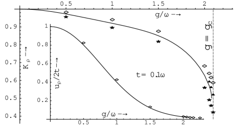
FIG. 3.: Coupling dependence of the Luttinger liquid parameters $u_{\rho}$ (charge velocity) and $K_{\rho}$ (correlation exponent) for the case $t=0.1\omega$. The diamonds and stars are the values of $K_{\rho}$ calculated from the finite-size scaling of the energy gaps $\Delta_{\text{ch}}$ and $\Delta_{1}$, respectively. The solid triangles are the $K_{\rho}$ values determined from (3). The solid curves are the results of strong coupling theory [3].

A theory for these nonlinear correction terms has been developed for the critical case [13, 21], namely $\Delta_{\text{ch}}\sim\frac{2\pi u_{\rho}}{N}\left[\frac{1}{4K_{\rho}}+\frac{A}{\log N}+\ldots\right]$ and $\Delta_{2}\sim\frac{2\pi u_{\rho}}{N}\left[K_{\rho}-\frac{3A}{\log N}+\ldots\right]$, where $A$ is a constant and $K_{\rho}=1/2$. By taking the combination

$$3\Delta_{\text{ch}}+\Delta_{2}\sim\frac{2\pi u_{\rho}}{N}\left[\frac{3}{4K_{\rho}}+K_{\rho}+\ldots\right],$$ (3)

the leading nonlinear correction is cancelled at $g=g_{\text{c}}$, the next correction being $O\left(\frac{1}{(\log N)^{2}}\right)$. For $t=\omega$ and $g=g_{\text{c}}$ $K_{\rho}=0.52$ is obtained if (3) is used to determine $K_{\rho}$. In comparison, values of 0.59 and 0.42 are obtained from the scaling of $\Delta_{\text{ch}}$ and $\Delta_{1}$, respectively. It might be expected that (3) should give better results for $K_{\rho}$ around the critical point than the scaling of $\Delta_{\text{ch}}$ or $\Delta_{1}$. The resulting values, plotted in Fig. 3, are in good agreement with strong coupling theory. To check the consistency of the transition with a K-T transition the value of $g$ at which $K_{\rho}$ (calculated using (3)) equals $\frac{1}{2}$ is listed in Table III. It can be seen that the transition is consistent with a K-T transition throughout the phase diagram.

TABLE III.: Transition point $g_{\text{c}}$ (as determined by the crossover of $\Delta_{\text{ch}}$ and $\Delta_{1}$) and $g^{*}$, the value of $g$ at which $K_{\rho}=\frac{1}{2}$, (where $K_{\rho}$ is calculated from (3)) for various hopping parameters $t$. The agreement between $g_{\text{c}}$ and $g^{*}$ is consistent with the transition being of the K-T type.

$t/\omega$	0.05	0.1	0.5	1	5	10
$g_{\text{c}}/\omega$	2.297(2)	2.093(2)	1.63(1)	1.61(1)	2.21(3)	2.79(5)
$g^{*}/\omega$	2.299	2.102	1.64	1.62	2.27	2.89

Finally, we consider the question of phonon softening and the mixing of phonon and fermion excitations. Fig. 4 shows the FSS of the energy gaps for a metallic case ($g<g_{\text{c}}$) with large hopping $t=5\omega$. Whilst $\Delta_{\text{ch}}$ is linear in $1/N$, $\Delta_{1}$ and $\Delta_{2}$ are highly nonlinear. This is because the lowest fermionic and bosonic, neutral excitations have the same quantum numbers, those of $\Delta_{1}$ and $\Delta_{2}$: The non-interacting fermionic gap $\frac{4\pi t}{N}$ only becomes less than the bare phonon frequency $\omega$ for $N\approx\frac{4\pi t}{\omega}\approx 60$ and thus $\Delta_{1}$ and $\Delta_{2}$ are predominantly 1- and 2- phonon excitations for small $N$ (flat in $1/N$), only becoming 1- and 2- particle-hole excitations (linear in $1/N$) for large $N$. Note that for these parameter values the phonons are softened—the renormalised phonon frequency is around half the bare phonon frequency $\omega$. It would be interesting to calculate the 1-phonon Green’s function to see if the phonons soften completely at the transition. The 2-phonon Green’s function could be used to study phonon anharmonicity.

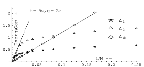
FIG. 4.: The energy gaps $\Delta_{\text{ch}}$, $\Delta_{1}$ and $\Delta_{2}$ as functions of $1/N$ for $t=5\omega$ in a metallic case $g=2\omega$. Dashed lines are straight lines through the origin. The gaps $\Delta_{1}$ and $\Delta_{2}$ are not linear in $1/N$ because in the adiabatic regime there is strong mixing between fermionic and phonon excitations. For systems of less than 20 sites the lowest excitations with quantum numbers $\hat{P}=\pm 1$ and $\hat{N}=N/2$ are predominantly 1- and 2- phonon excitations.

In conclusion, we have shown that, using a new variant of the DMRG, the phase boundary of the one-dimensional Holstein model of spinless fermions can be accurately determined. The transition is consistent with a K-T transition over a wide range of adiabacity. In the antiadiabatic limit the phase boundary and Luttinger liquid parameters agree well with strong coupling theory. In the adiabatic limit the phase boundary lies close to a curve predicted by renormalization group arguments. Challenges that remain include: 1) finding a method of cancelling nonlinear corrections to scaling, and hence accurately calculating the correlation exponent $K_{\rho}$, in the whole of the Luttinger liquid regime; 2) developing a theory of FSS when the conformally invariant field is coupled to a dispersionless field with a gap in order to explain the nonlinear scaling in Fig. 4; and 3) a detailed investigation of phonon softening and anharmonicity.

This work was supported by the Australian Research Council. We thank J. Voit, H. Eckle, E. Jeckelmann, T. Xiang, H. Fehske and V. Kotov for useful discussions. Calculations were performed at the New South Wales Centre for Parallel Computing.

REFERENCES

- [1] Email address: ph1rb@newt.phys.unsw.edu.au
- [2] A. S. Alexandrov and N. Mott, Polarons and Bipolarons (World Scientific, Singapore, 1995).
- [3] R.H. McKenzie, C.J. Hamer and D.W. Murray, Phys. Rev. B 53, 9676 (1996).
- [4] R.H. McKenzie and J.W. Wilkins, Phys. Rev. Lett. 69, 1085 (1992), and references therein.
- [5] J.E. Hirsch and E. Fradkin, Phys. Rev. B 27, 4302 (1983).
- [6] G. Benfatto, G. Gallavotti and J. L. Lebowitz, Helv. Phys. Acta 68, 312 (1995).
- [7] R. J. Bursill, unpublished.
- [8] S. R. White, Phys. Rev. Lett. 69, 2863 (1992); Phys. Rev. B 48, 10 345 (1993); G. A. Gehring, R. J. Bursill and T. Xiang, Acta Physica Polonica 91, 105 (1997).
- [9] L. G. Caron and S. Moukouri, Phys. Rev. Lett. 76, 4050 (1996); Phys. Rev. B 56, R8471 (1997).
- [10] E. Jeckelmann and S. R. White, Phys. Rev. B 57, 6376 (1998).
- [11] C. Zhang, E. Jeckelmann and S. R. White, Phys. Rev. Lett. 80, 2661 (1998).
- [12] It will be shown (see Fig. 4) that, in general, the lowest two neutral excitations are neither purely fermionic (particle-hole) nor phonon excitations and so we denote them 1- and 2- “photon” excitations, as they are the excitations that would be seen if one- and two- photon absorption experiments were carried out on a system described by the model. In the spin language of Nomura and Okamoto (ref. [14]), and are known as the Néel and dimer gaps.
- [13] I. Affleck et al., J. Phys. A 22, 511 (1989); K. Okamoto and K. Nomura, Phys. Lett. A 169, 433 (1992).
- [14] K. Nomura and K. Okamoto, J. Phys. A 27, 5773 (1994).
- [15] This is different from determining the transition point in the frustrated Heisenberg model which is spin rotationally symmetric ( for all ). For that model the crossover point is defined by .
- [16] L. G. Caron and C. Bourbonnais, Phys. Rev. B 29, 4230 (1984).
- [17] C. Q. Wu, Q. F. Huang, and X. Sun, Phys. Rev. B 52, 15683 (1995).
- [18] J. Voit, Rep. Prog. Phys. 58, 977 (1995).
- [19] J. L. Cardy, J. Phys. A 17, L385 (1984).
- [20] R. Shankar, Int. J. Mod. Phys. 4, 2371 (1990).
- [21] J. L. Cardy, J. Phys. A 20, 5039 (1987).