Identification of excitons in conjugated polymers: a density matrix renormalisation group study

Abstract

This work addresses the question of whether low-lying excitations in conjugated polymers are comprised of free charge-carriers or excitons. States are characterised as bound or unbound according to the scaling of the average particle-hole separation with system size. We critically examine other criteria commonly used to characterise states. The polymer is described by an extended Hubbard model with alternating transfer integrals. The model is solved by exact diagonalisation and the density matrix renormalisation group (DMRG) method. We demonstrate that the DMRG accurately determines excitation energies, transition dipole moments and particle-hole separations of a number of dipole forbidden ($A_{g}$) and dipole allowed ($B_{u}$) states.

Within a parameter regime considered reasonable for polymers such as polyacetylene, it is found that the charge gap, often used to define the exciton binding energy, is not a good criterion by which to decide whether a state is bound or unbound. The essential non-linear optical state $mA_{g}$ is found to mark the onset of unbound excitations in the $A_{g}$ symmetry sector. In the $B_{u}$ symmetry sector, on the other hand, it is found that all low lying states are unbound and that there is no well defined $nB_{u}$ state. That is, the $1B_{u}$ state marks the onset of unbound excitations in this sector.

]

I Introduction

The current interest in conjugated polymers lies to a large extent in their optical properties [3]. Conjugated polymers exhibit strong luminescence, and large and ultrafast nonlinear optical (NLO) response [4]. This has lead to technological opportunities and, for instance, polymer light-emitting diodes are now widely produced [5]. These optical properties are associated with the delocalised $\pi$-electron system of the conjugated polymers and, in particular, the low-lying excitations. However, the nature of these excitations is not fully understood, and has been a subject for fundamental research on conjugated polymers in recent years [3].

A central issue is whether low-lying excitations are comprised of free charge-carriers or excitons. If the Coulomb interaction between the oppositely charged particles and holes is strong, excitons are formed, i.e. bound particle-hole pairs, in which the motions of the particle and the hole are strongly correlated. On the other hand, if the Coulomb interaction is effectively screened, then the particles and holes are only very weakly bound and move essentially independently as free charge-carriers.

Different criteria have been used in the literature to discriminate between the states, leading to contradictory conclusions concerning the nature of the low-lying states. Some commonly used criteria are: the charge gap, $E_{\text{g}}$ [6, 7, 8]; and the essential NLO states, $mA_{g}$ and $nB_{u}$ [9, 10].

The charge gap is defined as the sum of the energies for removing and adding an electron to the neutral system:

$$E_{\text{g}}=E(N+1)+E(N-1)-2E(N).$$ (1)

where $E(N)$ refers to the ground state energy of the neutral system (where the band is half filled). For the Hubbard model with only on-site Coulomb interaction, the charge gap coincides with the lowest optical excitation, i.e. the optical gap [6]. This is, of course, also true for the tight-binding (or Hückel) model, which is an independent-electron model, where the charge gap is the onset of the delocalised states in the conduction band. However, this is generally not true in the case of longer range Coulomb interactions since there are states below the charge gap. It has been argued that these states are exciton states since they, for instance, appear energetically within the tight-binding band gap. Thus, the charge gap has been used to discriminate between the states: states below the charge gap correspond to excitons and states above the charge gap correspond to free charge-carriers. Consequently, for a state of energy $E$, the binding energy $E_{\text{b}}$ is defined as

$$E_{\text{b}}\equiv E_{\text{g}}-E.$$ (2)

We believe that this criterion can be seriously criticised: (i) the charge-gap energy is in general not an eigenenergy of the system, but rather mixes ground state energies of three, all differently charged, systems; (ii) the criterion does not distinguish between different symmetry sectors; and (iii) the criterion does not directly measure the motion of particles and holes, but is based on total energies only. In this work, we have directly calculated the relative motion of particles and holes for different states in each symmetry sector in order to identify excitons.

It should be noted that the use of the Hartree-Fock bandgap in the literature [7] is merely an approximate way of calculating the charge gap. This follows directly from Koopmans’ theorem, and we will therefore not treat the Hartree-Fock bandgap as separate criterion for excitons. It is well known that the Hartree-Fock bandgap systematically overestimates the true charge gap.

In works on NLO properties of conjugated polymers the most important channels for such processes have been identified [11, 12, 13, 14], leading to a phenomenological model for third-order nonlinearity that is based on only the four most essential states [9]. These states are the ground state $1A_{g}$, the lowest dipole allowed state $1B_{u}$, the $mA_{g}$ and the $nB_{u}$. The $mA_{g}$ is defined as the state which has the strongest dipole [15] coupling (or transition moment) to the $1B_{u}$, and the $nB_{u}$ is defined as the state which has the strongest dipole coupling to the $mA_{g}$, apart from the $1B_{u}$.

In addition, it was found that there is sudden increase in the particle-hole separation at the $mA_{g}$ and the $nB_{u}$, i.e. all states below these states have more tightly bound particles and holes [9]. It has therefore been argued that the $mA_{g}$ and the $nB_{u}$ are the lowest lying free charge-carrier states and useful criteria for the identification of excitons. The binding energy is defined analogously to (2), but with the charge gap replaced with the $mA_{g}$ or $nB_{u}$ energy depending on which symmetry sector is of interest.

Although intriguing, it is not clear that states below the $mA_{g}$ and the $nB_{u}$ really correspond to excitons. The smaller particle-hole separation may simply be a consequence of system confinement. In principle one needs to study an infinite system to resolve this issue, whereas the results of [9] pertain to an oligomer of $N=8$ carbon atoms. Another approach is to look at how the particle-hole separation scales with the system size $N$. In this work, we have calculated the particle-hole separation for different system sizes. The particle-hole separation scales differently for free charge-carriers and bound states.

In another study, the particle-hole separation was studied as a function of system size [7], with electron correlation treated within the singly excited configuration-interaction (SCI) approximation. It was found that states of energy significantly below (above) the Hartree-Fock band gap were bound (unbound). Excitons are many body excitations and, for instance, it has been found that the exciton binding energy is sensitive to the inclusion of higher-order correlation through perturbation theory [16, 17]. It is therefore important to treat the electron correlation accurately when assessing exciton criteria. In this work, we have used exact diagonalisation of the Hamiltonian for systems ($N\leq 10$), and the Density Matrix Renormalisation Group method for longer systems ($N\leq 50$).

The methodology of this work is outlined in Sec. II, which contains definitions of calculated quantities and a description of the computational methods. The model Hamiltonian is defined in Sec. II A, particle-hole separation definitions are given in Sec. II B where the basis of the scaling analysis is outlined, the ionicity is defined in Sec. II C and the numerical solution of the model is described in Sec. II D. A more detailed derivation of the scaling behaviour in the non-interacting limit is given in Appendix A. Results are presented and discussed in Sec. III. The accuracy of the DMRG method is demonstrated in Sec. III A, the energy spectra and transition moments are given in Sec. III B, results for the particle-hole separation follow in Sec. III C, whilst ionicity results are given in Sec. III D. Finally, conclusions are given in Sec. IV.

II Methodology

A Model

As a generic model for conjugated polymers we study the extended Hubbard model with alternating hopping integrals and on-site and nearest-neighbour electron-electron interactions:

$$\hat{H} \equiv -t\sum_{i,\sigma}[1-(-1)^{i}\delta](\hat{c}_{i\sigma}^{\dagger}\hat{c}_{i+1\sigma}+\mbox{ h.c.})+$$ (4)

$$\frac{U}{2}\sum_{i}(\hat{n}_{i}-1)(\hat{n}_{i}-1)+V\sum_{i}(\hat{n}_{i}-1)(\hat{n}_{i+1}-1),$$

where $\hat{c}_{i\sigma}$ annihilates a $\pi$-electron with spin $\sigma$ on site $i$ and $\hat{n}_{i}$ is the occupation number operator for site $i$. We have studied systems with an even number of sites $N$, and open boundary conditions. The Hamiltonian is a paradigm for conjugated polymers in which excitons can exist.

For convenience we take $t=1$, which sets the energy scale. Values for the dimerisation in the range 0.07–0.15 have been proposed for polyacetylene, polydiacetylene, and poly(para-phenylenevinylene) [18, 6]. We choose $\delta=0.1$ as a typical value for conjugated polymers. Optical absorption data suggest a $U$ value of 2.25–2.75 [19], whereas ab initio calculations suggest a slightly higher value of 3.6 [20]. We have taken $U=3$ as a reasonably realistic value. For the nearest neighbour interaction we use the standard value $V=0.4U$ [9, 6]. Thus, the chosen values of the parameters are: $t=1$, $\delta=0.1$, $U=3$, and $V=1.2$. These values are used throughout the paper, unless otherwise stated.

Besides conserving the total number of particles, the Hamiltonian possesses spatial symmetry, $\hat{C}_{2h}\in\{A_{g},B_{u}\}$, charge conjugation symmetry, $\hat{J}\in\{+,-\}$, and spin symmetry, e.g. $\hat{S}\in\{0,1,2\ldots\}$ [21]. In this paper we are concerned with neutral, singlet states (with a half-filled band and $\hat{S}=0$), except for the charged states used in determining $E_{\text{g}}$. The singlet ground state is even under spatial inversion and charge conjugation, and is denoted $1^{1}A_{g}^{+}$, or simply $1A_{g}$. For this work we only need to consider the ground state symmetry sector and the sector to which it is dipole coupled. Since the dipole operator is odd under inversion and charge conjugation, states in the dipole coupled sector are denoted $j^{1}B_{u}^{-}$, or simply $jB_{u}$, where $j$ is the state number.

B Particle-hole separation

In this paper, we consider the relative motion of particles and holes as a direct way of identifying excitons. In particular, we calculate the average particle-hole separation. Excitons have small particle-hole separations which remain finite as the system size is increased. By contrast, the average separation between two free charge-carriers increases indefinitely with system size. Indeed, for a completely independent particle and hole, each with a uniform probability ($1/N$) of being on any given site, the leading term in the average separation is proportional to $N$.

In reference [9] Guo et al. used the density-density correlation function $C(i,j)$ as a signifier which distinguishes bound and unbound states:

$$C(i,j)\equiv\left\langle(\hat{n}_{i}-\left\langle\hat{n}_{i}\right\rangle)(\hat{n}_{j}-\left\langle\hat{n}_{j}\right\rangle)\right\rangle.$$ (5)

$C(i,j)$ correlates a charge fluctuation on site $i$ to a charge fluctuation on site $j$. A positive value means that an excess (deficit) of charge on site $i$ correlates with an excess (deficit) on site $j$. A negative value correlates an excess with a deficit. In the context of excitons, the concept of quasi-particles is a way of representing an aggregation of electrons which leads to an excess of charge in a region, which may extend over several sites. Likewise, a hole represents deficit of charge. Now, for sufficiently large $N$, $C(i,j)$ is negative (positive) for $|i-j|$ odd (even). We thus consider the odd distance contributions when defining the probability distribution from which to measure the separation of particles and holes. Other definitions, utilising both positive and negative contributions, or $|C(i,j)|$ are possible, and yield the same qualitative results.

In [9] it was found that there is a noticeable change in the nature of the decay of $C(i,j)$ at the $mA_{g}$ and $nB_{u}$, the particle-hole separation being considerably larger than for the lower lying states. However, calculations were restricted to $N=8$. We have used the DMRG method to study substantially larger systems (up to $N=50$). Most importantly, this makes it possible to discriminate between bound and unbound states from the scaling of $C(i,j)$ or the particle-hole separation with $N$.

We define an averaged [22], centered correlation function for a system of size $N$ with open boundary conditions as:

$$C_{N}(l)\equiv\left\{\begin{array}[]{ll}C(\frac{N-l}{2},\frac{N+l}{2})&\mbox{$l$ even}\\ \frac{1}{2}\left[C(\frac{N-l+1}{2},\frac{N+l+1}{2})+C(\frac{N-l-1}{2},\frac{N+l-1}{2})\right]&\mbox{$l$ odd.}\\ \end{array}\right..$$ (6)

As discussed, we define the average particle-hole separation (in units of chemical bonds) by regarding the negative values of $C_{N}(l)$ as a probability distribution viz.

$$\left\langle l\right\rangle_{N}\equiv\frac{\sum_{l=0}^{N-1}l(|C_{N}(l)|-C_{N}(l))}{\sum_{l=0}^{N-1}(|C_{N}(l)|-C_{N}(l))}.$$ (7)

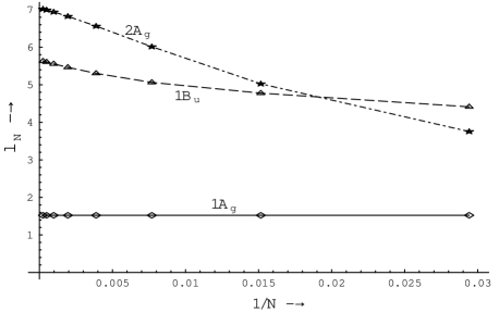
FIG. 1.: Particle-hole separation $\left\langle l\right\rangle_{N}$ of the $1A_{g}$, $2A_{g}$ and $1B_{u}$ states in the non-interacting limit ($U=V=0$) plotted as a function of $1/N$.

It is instructive to consider the two extreme cases of very weak and very strong electron-electron interaction, since the identification of bound and unbound states is unambiguous in these cases. In the non-interacting limit ($U=V=0$), we combine exact analytical results with exact diagonalisations of systems of up to 4098 sites in order to determine the scaling of the correlation function and particle-hole separation with $N$. Details are given in Appendix A. The main point is that, as can be seen from Fig. 1, the ground state ($1A_{g}$) and the unbound states ($1B_{u}$ and $2A_{g}$) have particle-hole separations which scale very differently with $N$. For the ground state we have exponential convergence

$$\left\langle l\right\rangle_{N}=a\left[1+O\left(e^{-\alpha N}\right)\right],$$ (8)

and for the unbound excited states we have very slow convergence

$$\left\langle l\right\rangle_{N}=b\left[1+O\left(N^{-1}\right)\right].$$ (9)

In the limit of strong interactions, ($U,V\gg t$), it was shown by Guo et al. [9] that the states can be identified solely from their total energy. At $t=0$, the analysis is trivial: A particle (hole) is a doubly-occupied (empty) site. The ground state has zero energy, bound states occur at $U-V$, and unbound states at $U$. Since the Hamiltonian consists only of the $U$-$V$ potential, the bound states have a particle and a hole next to one another, the correlation function vanishes for $l>1$, and the particle-hole separation converges immediately with $N$, i.e. $\left\langle l\right\rangle_{N}\equiv 1$. For unbound states, at energy $U$, it is easy to show that $\left\langle l\right\rangle_{N}$ increases linearly with $N$, i.e. as for independent particles and holes.

In addition to the correlation function, we consider a reduced correlation function: the difference between the correlation function of an excitation, $C_{N}(l)$, and that of the ground state, $C_{N}^{\text{(GS)}}(l)$:

$$C_{N}^{\text{(red)}}(l)\equiv N\left[C_{N}(l)-C_{N}^{\text{(GS)}}(l)\right].$$ (10)

The motivation for studying $C_{N}^{\text{(red)}}(l)$ is that it only measures changes in the charge fluctuations induced by an excitation. That is, the effect of creating particles and holes, whose motion we are interested in. By analogy with (7), we also define a reduced particle-hole separation $\left\langle l\right\rangle_{N}^{\text{(red)}}$.

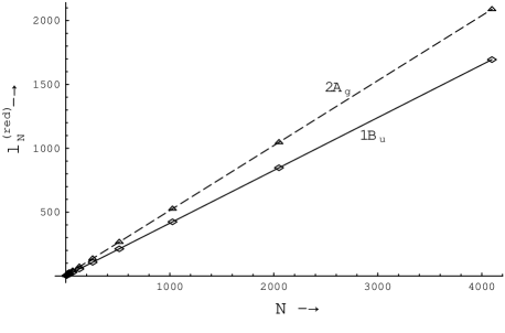
FIG. 2.: Reduced particle-hole separation $\left\langle l\right\rangle^{\text{(red)}}$ of the $1B_{u}$ and $2A_{g}$ states in the non-interacting limit ($U=V=0$) plotted as a function of $N$.

In the non-interacting case, the reduced particle-hole separation for unbound states scales linearly with $N$, as shown in Fig. 2. As mentioned above, this is how the separation of a completely independent particle and hole scale. In the strongly correlated limit, $C_{N}^{\text{(GS)}}(l)\equiv 0$ and so $\left\langle l\right\rangle_{N}^{\text{(red)}}\equiv\left\langle l\right\rangle_{N}$ and hence $\left\langle l\right\rangle^{\text{(red)}}_{N}\equiv 1$ for bound states and $\left\langle l\right\rangle^{\text{(red)}}_{N}\propto N$ for unbound states. That is, unbound states scale in the same way in both limits. This suggests that, for general interaction strength, the reduced particle-hole separation scales linearly for unbound states.

In summary, for unbound states, the particle-hole separation $\left\langle l\right\rangle_{N}$ converges slowly with $N$ and the reduced particle-hole separation $\left\langle l\right\rangle_{N}^{\text{(red)}}$ diverges linearly. By contrast, for bound states, both $\left\langle l\right\rangle_{N}$ and $\left\langle l\right\rangle_{N}^{\text{(red)}}$ converge rapidly to a finite value.

C Ionicity

In the limit of strong electron-electron interaction, $U\gg t$, the ground state is a pure spin-density-wave, i.e. it is solely a linear combination of covalent configurations (or Slater determinants), where there is exactly one electron on each site. It is therefore natural, in this limit, to define a particle as a doubly occupied site, and a hole as an unoccupied site. Configurations which have particles and holes are referred to as ionic. A general state can be written as $\Psi=\Psi^{\text{(covalent)}}+\Psi^{\text{(ionic)}}$.

Following [13], we define the ionicity as the number of particle-hole pairs [23]. Thus, single particle-hole pair excitons are constructed from singly ionic configurations, biexcitons are constructed from doubly ionic configurations etc. The ionicity of a state is defined as the expectation value of the ionicity operator $\hat{I}$:

$$\hat{I} = \frac{1}{2}\sum_{i}(\hat{n}_{i}-1)^{2}.$$ (11)

In addition to the ionicity, we have calculated the average ionic particle-hole separation $\left\langle l\right\rangle_{N}^{\text{(ionic)}}$ by considering only the ionic part of the wavefunction. In contrast to $\left\langle l\right\rangle_{N}$, $\left\langle l\right\rangle_{N}^{\text{(ionic)}}$ allows us to probe changes within $\Psi^{\text{(ionic)}}$ alone, rather than at the same time taking into account a change in the relative weights of $\Psi^{\text{(covalent)}}$ and $\Psi^{\text{(ionic)}}$.

D Computational methods

Equation (4) can be comfortably solved by exact diagonalisation for systems of up to $N=12$ sites. For longer chains we turn to the Density Matrix Renormalisation Group (DMRG) method [24]. The DMRG has been applied to (4) in calculations of ground state and triplet energies [25], charge densities [25], the charge gap and $1B_{u}$ energies [6, 26], the $2A_{g}$ energy [26], polarisabilities [27], and oscillator strengths [28].

In this work we apply an infinite lattice DMRG algorithm [24] to find the charge gap and a number of $A_{g}$ and $B_{u}$ states of (4). In addition to excitation energies, we find the transition dipole moments between the $A_{g}$ and $B_{u}$ states as well as the density-density correlation function (6) and hence the particle-hole separation (7) and reduced separation $\left\langle l\right\rangle_{N}^{\text{(red)}}$. At each iteration the superblock consists of a system block, an environment block and two extra sites. The initial system and environment blocks consist of two sites. The system and environment blocks are increased by two sites at a time until a superblock of $N=50$ sites is reached. We retain $m=230$ density matrix eigenstates in the basis truncation procedure.

The system, environment and super block Hamiltonians and density matrices are block diagonalised using the total particle number $\hat{N}$ and total $z$-spin $\hat{S}^{z}$ operators. States from different symmetry sectors are found by projecting trial states from the iterative, sparse matrix diagonalisation procedure into the correct symmetry sector by means of the operators $\hat{C}_{2h}$, $\hat{J}$ and the spin-parity operator $\hat{P}$ [29]. Because the density matrix commutes with the block $\hat{J}$ and $\hat{P}$ operators, the superblock states calculated are exact eigenstates of $\hat{J}$ and $\hat{P}$ at all stages of the calculation. They are also exact eigenstates of $\hat{C}_{2h}$ by construction because the environment block is the reflection of the system block. We check the DMRG program by ensuring that it reproduces the results of the exact diagonalisation program for the first two iterations. The exact diagonalisation program itself reproduces the $N=8$ site results from [9].

III Results and discussion

A Accuracy of the DMRG calculations

We begin with the non-interacting limit ($U=V=0$), where we have performed separate exact diagonalisations for long chains in order to evaluate the DMRG accuracy. The non-interacting case is of particular interest since it gives a worst case accuracy. Errors are expected to be smaller in the interacting case where particles are more localised in position space, the DMRG becoming exact in the atomic ($t=0$) limit.

In the DMRG calculations the initial two systems ($N=6,10$) are treated exactly. The errors for these systems are merely a result of the limited precision of the sparse matrix diagonalisation algorithm (the accuracy could be increased by running the programs at higher precision). The DMRG truncation error sets in at $N=14$ where the relative error is $\sim 10^{-5}$. The error increases with system size and is $\sim 10^{-4}$ for $N=30$–$50$.

In addition to excitation energies, it is important to look at quantities such as transition moments and particle-hole separations, which pertain to the wavefunction rather than the energy. The truncation error for transition moments is $\sim 10^{-3}$ for $N=30$–$50$, i.e. one order of magnitude larger than for excitation energies, but well within what is acceptable for our purposes. The particle-hole separations have similar errors to the transition moments.

The DMRG is a truncated basis method with systematically reducible error. In the interacting case it is important to test the accuracy of calculations by varying the single source of error, the truncation parameter $m$, and checking for convergence. We asses the error by running the program for a number of values of $m$. Convergence results for a number of quantities are given in Table I for the $N=50$ site system. It is found that the ground state energy converges to 5 or 6 figures and gaps are resolved to within 0.01% for the charge gap and $1B_{u}$ states, with slower convergence for the higher excitations where errors range up to one or two percent. The errors in transition dipole moments are larger but are still small enough to make a clear identification of the essential NLO states. Errors range from around 0.5% for the $1A_{g}\rightarrow 1B_{u}$ transition to 1–2% for the $mA_{g}\rightarrow 1B_{u}$ transition. The errors in the particle-hole separations are found to range from 0.1% for the $1A_{g}$ state to 1–3% for the higher excitations. Convergence is sufficiently good to allow the clear classification of states as bound or unbound on the basis of the scaling of the particle-hole separation.

TABLE I.: The ground state energy $(1A_{g})$, the charge gap $E_{\text{g}}$, the $1B_{u}$ and $4A_{g}$ energy gaps, various transition moments $\left\langle jB_{u}|\hat{\mu}|1A_{g}\right\rangle$ and particle-hole separations $\left\langle l\right\rangle_{50}$ for the $N=50$ site system calculated using the DMRG for a number of truncation parameter values $m$.

	Energy				$\left\langle jB_{u}|\hat{\mu}|mA_{g}\right\rangle$		$\left\langle l\right\rangle_{50}$
$m$	$1A_{g}$	$E_{\text{g}}$	$1B_{u}$	$4A_{g}$	$1B_{u}$	$3B_{u}$	$2B_{u}$	$4B_{u}$
64	$-$102.97649	1.2190	1.1122	1.1761	1.479	9.472	1.883	1.942
100	$-$102.97925	1.2212	1.1058	1.5455	7.151	6.599	2.018	1.726
150	$-$102.97969	1.2213	1.1044	1.4801	7.065	6.847	2.061	1.632
185	$-$102.97996	1.2218	1.1026	1.3855	6.962	7.297	2.078	1.602
230	$-$102.98002	1.2218	1.1025	1.3431	6.945	7.330	2.085	1.596

B Excitation energies and transition moments

The evolution of the energy spectra with system size is shown in Fig. 3 and Fig. 4 for the $A_{g}$ and $B_{u}$ sectors respectively. The charge gap is also shown for comparison. There is exactly one excitation below the charge gap for all system sizes in the $B_{u}$ symmetry sector, and for most systems in the $A_{g}$ sector. The $3A_{g}$ drops below the charge gap for $N=42$–$50$.

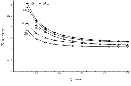
FIG. 3.: Excitation energies (relative to the $1A_{g}$) in the $A_{g}$ symmetry sector as a function of $N$. The charge gap (dashed line) is shown for comparison.

Transition moments between various $A_{g}$ states and the $1B_{u}$ are given in Table II. The $mA_{g}$ can be identified as the $5A_{g}$ for $N=10$–$50$. The transition moment with the $2A_{g}$ increases with system size, while transition moments with the $3A_{g}$ and the $4A_{g}$ decrease for $N\geq 22$. The charge gap is always below the $mA_{g}$ energy so the charge gap criterion will give lower exciton binding energies than the $mA_{g}$ criterion.

TABLE II.: Transition moments $\left\langle jA_{g}|\hat{\mu}|1B_{u}\right\rangle$ for various states $jA_{g}$ and system sizes $N$.

	$\left\langle jA_{g}|\hat{\mu}|1B_{u}\right\rangle$
$N$	$1A_{g}$	$2A_{g}$	$3A_{g}$	$4A_{g}$	$5A_{g}$
6	1.529	0.239	0.185	2.697	0.195
10	2.144	0.664	0.000	0.970	4.006
14	2.613	1.210	0.179	2.089	4.879
18	2.987	1.794	0.270	2.592	5.691
22	3.300	2.369	0.241	2.779	6.384
26	3.548	2.924	0.173	2.770	6.920
30	3.789	3.408	0.112	2.639	7.290
34	4.071	3.706	0.069	2.421	7.464
38	4.303	3.989	0.046	2.162	7.543
42	4.528	4.203	0.043	1.526	7.627
46	4.636	4.703	0.046	1.786	7.594
50	4.831	4.899	0.058	1.603	7.521

The transition moments for the identification of the $nB_{u}$ are given in Table III. There are two qualitative differences between these transition moments and those used for the identification of the $mA_{g}$ (Table II). Firstly, while the state number of the $mA_{g}$ is basically constant ($m=5$, apart from $N=6$), the state number of the $nB_{u}$ changes with the system size when the definition of Sec. I is applied. It is the $5B_{u}$ at N=6, the $4B_{u}$ at $N=10,14$ and the $2B_{u}$ at $N=18,22,26$.

TABLE III.: Transition moments $\left\langle jB_{u}|\hat{\mu}|mA_{g}\right\rangle$ for various states $jB_{u}$ and system sizes $N$.

	$\left\langle jB_{u}|\hat{\mu}|mA_{g}\right\rangle$
$N$	$1B_{u}$	$2B_{u}$	$3B_{u}$	$4B_{u}$	$5B_{u}$	$6B_{u}$
6	2.697	0.908	0.281	1.916	2.135	0.041
10	4.006	2.059	0.391	3.977	0.235	1.735
14	4.879	3.524	0.016	4.640	0.287	2.446
18	5.691	5.278	0.845	4.771	3.299	1.291
22	6.384	6.892	2.664	0.396	5.997	2.207
26	6.920	6.860	6.585	1.822	0.987	6.361

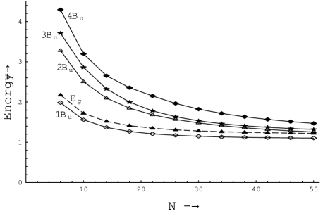
FIG. 4.: Excitation energies (relative to the $1A_{g}$) in the $B_{u}$ symmetry sector as a function of $N$. The charge gap (dashed line) and is shown for comparison.

Secondly, for many system sizes, the $nB_{u}$ is ill-defined in the sense that there are several transition moments close to the maximum value and to that of the $nB_{u}$. For instance, at $N=18$, the $1B_{u}$, $2B_{u}$ and $4B_{u}$ have very similar transition moments; at $N=22$, the $1B_{u}$, $2B_{u}$ and $5B_{u}$; and at $N=26$, the $1B_{u}$, $2B_{u}$, $3B_{u}$, and $6B_{u}$. It was found in [9] that conduction-band states had strong dipole coupling to several neighbouring conduction-band states in the dipole coupled symmetry sector. This was seen to distinguish band-to-band transitions from transitions involving excitons. If the $mA_{g}$ is the onset of the conduction-band, i.e. the lowest lying unbound $A_{g}$ state, then our results imply that the $1B_{u}$ is the onset of the conduction-band in the $B_{u}$ symmetry sector. A stronger argument, based on the scaling of the particle-hole separation, is given in Sec. III C.

C Particle-hole separation

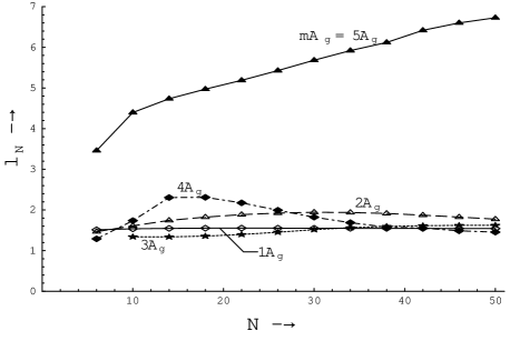
FIG. 5.: Particle-hole separation $\left\langle l\right\rangle_{N}$ of the $A_{g}$ states as a function of $N$. The plot shows all states up to the $mA_{g}$.

The particle-hole separation $\left\langle l\right\rangle_{N}$ of the $A_{g}$ states is plotted as a function of $N$ in Fig. 5. We see that the $mA_{g}$ displays completely different behaviour from all the lower lying $A_{g}$ states. For the lower states, the average separation converges rapidly to the ground state (bulk limit) value of around 1.3 chemical bonds [30]. By contrast, for the $mA_{g}$ the separation is significantly larger for all $N$, exhibiting a far stronger $N$ dependence, and converging to a different limit from the bulk limit if converging at all. It follows that the $A_{g}$ states below the $mA_{g}$ are bound and the $mA_{g}$ is unbound.

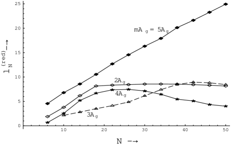
FIG. 6.: The reduced particle-hole separation $\left\langle l\right\rangle^{\text{(red)}}_{N}$ of the $A_{g}$ states as a function of $N$. The plot shows all states up to the $mA_{g}$.

The striking difference between the $mA_{g}$ and the lower $A_{g}$ states is also borne out in the behaviour of the reduced particle-hole separation $\left\langle l\right\rangle^{\text{(red)}}_{N}$ depicted in Fig. 6. The reduced separation of the $mA_{g}$ scales linearly with $N$, i.e. as for completely independent particles and holes. For $N=50$, the average separation is around 25 chemical bonds. The lower states, on the other hand, all have bounded separation. For instance, for the $2A_{g}$ $\left\langle l\right\rangle^{\text{(red)}}_{N}$ scales linearly up to $N=18$ where it levels off at around 8 chemical bonds. The interpretation of this is clear: the $2A_{g}$ is comprised of excitons with an average size of 8 bonds. When the system reaches a sufficiently large size the separation settles at the intrinsic average size of the exciton. For smaller systems, around or below the exciton size, the average separation is dictated by the system confinement.

In summary, the $A_{g}$ states below the $mA_{g}$ are bound, and the $mA_{g}$ is the lowest lying free charge-carrier state in this symmetry sector. We have only performed calculations for up to $N=50$, and thus in principle we cannot be certain that the reduced separation of the $mA_{g}$ does not eventually taper off. However, it is clear from our calculations that the $mA_{g}$ behaves as a free charge-carrier state for systems of up to 50 sites. If an upper bound does exist, then the $mA_{g}$ must be extremely weakly bound. The $mA_{g}$ energy is therefore a good reference energy when calculating binding energies in this symmetry sector. The charge gap, on the other hand, falls amongst the bound states. Some of the bound states are above the charge gap, while others are below. Thus, the charge gap fails to discriminate between bound and unbound states.

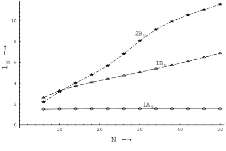
FIG. 7.: Particle-hole separation $\left\langle l\right\rangle_{N}$ of the $B_{u}$ states as a function of $N$. The $1A_{g}$ state is plotted for reference.

We now turn to the dipole-allowed ($B_{u}$) symmetry sector. The particle-hole separation is shown in Fig. 7. The separations depend strongly on $N$, indicating that there are no bound states in this sector. This is confirmed by the reduced particle-hole separation, shown in Fig. 8: The $1B_{u}$ scales almost perfectly linearly with $N$ and the $2B_{u}$ increases at least as rapidly over the plotted range. This explains the absence of a well defined $nB_{u}$ state above the $1B_{u}$ (see Sec. III B). That is, the $1B_{u}$ is the lowest unbound state in the $B_{u}$ sector. We note that the charge gap lies above the $1B_{u}$, incorrectly suggesting that the $1B_{u}$ is a bound state (see Fig. 4). As was the case for the $A_{g}$ sector, the charge gap is not a useful criterion for determining whether states are bound and unbound in this symmetry sector.

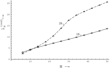
FIG. 8.: The reduced particle-hole separation $\left\langle l\right\rangle^{\text{(red)}}_{N}$ of the $B_{u}$ states as a function of $N$.

D Ionicity

The ionicity gives additional insight into the nature of the low-lying states. It is instructive to first study a case of relatively strong Coulomb interaction ($U=10$, $V=4$). As seen in Fig. 9, there is a sudden jump in the ionicity at the $mA_{g}$, for which $\left\langle\hat{I}\right\rangle=1.4$. The ground state has an ionicity of 0.45, and an excitation to the $mA_{g}$ creates almost exactly one particle-hole pair. Lower lying states, on the other hand, follow a more continuous evolution with similar ionicity to that of the ground state. In fact, the ionicity decreases, the $(m-1)A_{g}$ being almost purely covalent. By contrast, there is no such jump in the $B_{u}$ symmetry sector at the $nB_{u}$. Instead all states have about the same ionicity, similar to that of the $mA_{g}$.

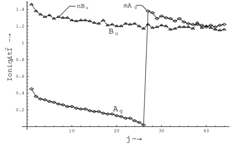
FIG. 9.: The ionicity of the $jA_{g}$ and $jB_{u}$ states for $U=10$, $V=4$, $N=10$.

For the weaker, more realistic, interaction (see Sec. II A), the ionicity is shown in Fig. 10. Although there are large quantitative differences, many qualitative features remain. In the $A_{g}$ sector, the ionicity decreases continuously up to the $mA_{g}$ where a distinct jump occurs. Again, the ionicity of the $B_{u}$ states remains constant at around the same value as the $mA_{g}$. There is, however, one qualitative change, namely that the spectrum above the $mA_{g}$ is now a mixture of states with high and low ionicity. A picture where the $mA_{g}$ is the onset of a band of states which are all unbound appears to be too simplistic, at least from the $N=10$ site data.

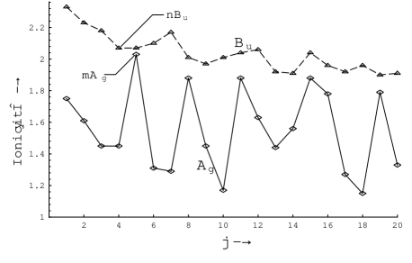
FIG. 10.: The ionicity of the $jA_{g}$ and $jB_{u}$ states for $U=3$, $V=1.2$, $N=10$.

The average ionic separation, shown in Table IV, also shows a jump at the $mA_{g}$, from slightly more than 2 for the lower states to 3.5. In the other symmetry sector, the maximum ionic separation is 3.8 for the $nB_{u}$. However, the jump is less pronounced since the lower states all have relatively large separations of around 3.0.

TABLE IV.: The average ionic separation of $jA_{g}$ and $jB_{u}$ states for $N=10$.

	$\left\langle l\right\rangle_{10}^{\text{(ionic)}}$
j	$A_{g}$	$B_{u}$
1	2.23	2.97
2	2.21	3.21
3	2.04	2.82
$4=n$	2.11	3.77
$5=m$	3.54	3.08

To conclude, the $mA_{g}$ excitation involves the creation of more particle-hole pairs than the lower lying states in the $A_{g}$ sector. Furthermore, the particle-hole pairs as less strongly bound. The large charge separation of the $mA_{g}$ is a result of two factors: a redistribution of weights in the wavefunction, from covalent to ionic configurations, and an increased charge separation within the ionic part of the wave function. By contrast, in the $B_{u}$ symmetry sector the difference between the $nB_{u}$ and the lower states is far less pronounced, a result which is consistent with the findings of Sec. III C.

IV Conclusions

In this paper we have studied the particle-hole separation in the fundamental model of conjugated polymers—the dimerised, extended Hubbard model—in order to critically assess criteria commonly used to determine whether excitations are excitonic or consist of uncorrelated particle-hole pairs. The chosen parameter values are typical values used to describe polymers such as polyacetylene within the model. The model was solved for the charge gap and a number of states in the ground state ($A_{g}$) and dipole allowed ($B_{u}$) symmetry sectors using the Density Matrix Renormalisation Group (DMRG) method for systems of up to $N=50$ sites. It was shown that the DMRG can be used to accurately compute energy gaps, transition dipole moments and particle-hole separations for these states, with relative errors ranging from a fraction of a percent for the lowest states to a few percent for higher states. The particle-hole separations of bound and unbound states were shown to scale differently with system size, a fact which can be used to discriminate between the states.

It was found that the charge gap, often used to define the binding energy of excitons, is not a useful criterion by which to decide whether a state is bound or unbound. The results for the scaling of the particle-hole separation show that there is an unbound state below the charge gap in the $B_{u}$ symmetry sector, and bound states states above the charge gap in the $A_{g}$ sector. Thus, it is possible to have states below the charge gap which are unbound, and states above the charge gap which are bound. In fact, the results were in keeping with the picture that the essential non-linear optical state $mA_{g}$ marks the onset of unbound states in the $A_{g}$ symmetry sector. On the other hand, in the $B_{u}$ sector it was found that all states were unbound for the parameters considered, and that there was no well defined $nB_{u}$ state. That is, the $1B_{u}$ state marks the onset of unbound excitations in the $B_{u}$ sector.

Finally, we note that, although the dimerised, extended Hubbard model is a fundamental model which is believed to provide a qualitative description of polymers such as polyacetylene, one needs to investigate the effects of long range Coulomb interactions, interchain coupling and electron-phonon effects before one can begin to make reliable statements about the nature of excitons in specific, real conjugated systems. We are currently developing efficient, vectorised DMRG codes with which we will be able to study these effects.

A Scaling of the correlation function and particle-hole separation in the non-interacting limit

In this appendix we present some results for the correlation functions of excited states of (4) in the non-interacting limit ($U=V=0$). In arriving at these results, we make use of well known analytical results for open and periodic systems and diagonalisations of open systems of up to 4098 sites.

The bulk correlation function is given by

$$C_{\infty}(l) \equiv \lim_{N\rightarrow\infty}C_{N}(l)$$ (A1)

$$= \left\{\begin{array}[]{ll}1/2&l=0\\ 0&l>0\mbox{, even}\\ -|F(l,\delta,+)|^{2}-|F(l,\delta,-)|^{2}&l\mbox{ odd,}\end{array}\right.$$ (A5)

where

$$F(l,\delta,\pm)\equiv\frac{1}{\pi}\int_{-\pi/2}^{\pi/2}e^{il\theta}\sqrt{\frac{\cos\theta\pm i\delta\sin\theta}{\cos\theta\mp i\delta\sin\theta}}\,d\theta$$ (A6)

For $0<\delta<1$, the model has a gap $\Delta=4\delta t$ and exponentially decaying correlations

$$C_{\infty}(l)\sim e^{-l/\xi}\mbox{ as }l\rightarrow\infty\mbox{ ($l$ odd),}$$ (A7)

with correlation length

$$\xi=\frac{1}{2\tanh^{-1}\delta}.$$ (A8)

For the ground state of a system of size $N$ we have

$$C_{N}^{\text{(GS)}}(l)\equiv C_{\infty}(l)\equiv 0\mbox{ for all $l$ even,}$$ (A9)

and for odd $l$, $C_{N}^{\text{(GS)}}(l)$ approaches $C_{\infty}(l)$ exponentially fast viz

$$C_{N}^{\text{(GS)}}(l)=C_{\infty}(l)\left[1+O\left(e^{-\alpha N}\right)\right]\mbox{ ($l$ odd),}$$ (A10)

for some positive constant $\alpha$ which is uniform over $l$. It follows that the ground state particle-hole separation converges rapidly, according to (8), where

$$a\equiv\lim_{m\rightarrow\infty}\frac{\sum_{l=1}^{m}(2l-1)\left|C_{\infty}(2l-1)\right|}{\sum_{l=1}^{m}\left|C_{\infty}(2l-1)\right|}$$ (A11)

is the particle-hole separation defined from the bulk correlation function (A1). This can be seen in Fig. 1 where $\left\langle l\right\rangle_{N}$ is plotted for the $1A_{g}$ state.

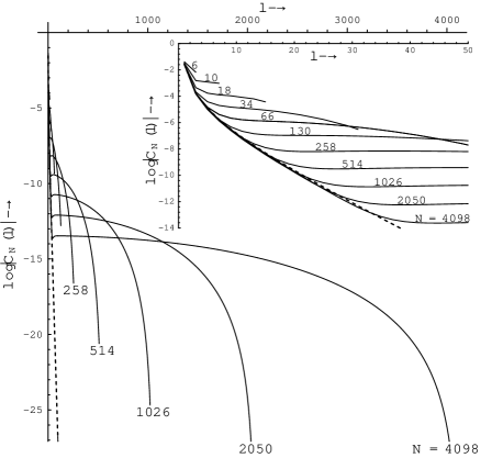
FIG. 11.: $\log|C_{N}(l)|$ for the $1B_{u}$ state as a function of $l$ for $N=$ 6, 10, 18, 34, 66, 130, 258, 514, 1026, 2050 and 4098 in the non-interacting case ($U=V=0$). Also plotted is $\log|C_{\infty}(l)|$, the bulk (ground state) value (dashed line). Only the odd values of $l$ are used. The inset shows the same plot on a smaller horizontal scale.

For the excited states the finite lattice correlation function $C_{N}(l)$ approaches the infinite lattice value $C_{\infty}(l)$ as $N\rightarrow\infty$ for any fixed $l$ [31]. However, as can be seen from Fig. 11, where we plot $\log|C_{N}(l)|$ for the $1B_{u}$ states as a function of $l$ for various values of $N$, the convergence is very slow. This is shown in Fig. 12, where we plot the reduced correlation function $C_{N}^{\text{(red)}}(l)$, defined by (10), as a function of $1/N$ for a number of values of $l$. We see clearly that the scaling behaviour of the excited state correlation function is

$$C_{N}(l)=C_{\infty}(l)+\frac{C^{\text{(red)}}_{\infty}(l)}{N}+\frac{g(l)}{N^{2}}+\ldots,$$ (A12)

where $C^{\text{(red)}}_{\infty}(l)$ is the limiting, reduced correlation function viz

$$C^{\text{(red)}}_{\infty}(l)\equiv\lim_{N\rightarrow\infty}C^{\text{(red)}}_{N}(l).$$ (A13)

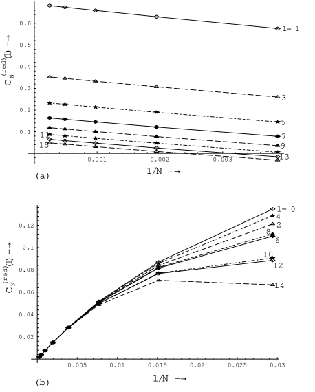
FIG. 12.: Reduced correlation function $C_{N}^{\text{(red)}}(l)$ for the $1B_{u}$ state as a function of $1/N$ for various (a) odd and (b) even values of $l$ in the non-interacting case ($U=V=0$).

Using a polynomial fit of the form (A12) and extrapolating to the $N=\infty$ limit, $C^{\text{(red)}}_{\infty}(l)$ is calculated and plotted in Fig. 13. We see that $C^{\text{(red)}}_{\infty}(l)$ decays exponentially with $l$, and vanishes for even $l$. In fact, the scaling form (A12) can be derived explicitly for the case of periodic boundary conditions, where it can be shown that

$$C^{\text{(red)}}_{\infty}(l)=\sqrt{C_{\infty}(l)}f(l)$$ (A14)

where the functions $f(l)$ and $g(l)$ rapidly approach non-zero constants as $l$ is increased (i.e. $C^{\text{(red)}}_{\infty}(l)$ decays exponentially and has correlation length $2\xi$). The functions $f$ and $g$, derived from the polynomial fit to (A12), are plotted in the inset of Fig. 13.

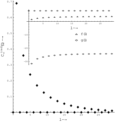
FIG. 13.: Limiting reduced correlation function $C_{\infty}^{\text{(red)}}(l)$ for the $1B_{u}$ state as a function of $l$ in the non-interacting case ($U=V=0$). The inset shows the scaling functions $f(l)$ and $g(l)$ ($f(l)$ is only defined for odd values of $l$ because $C_{\infty}^{\text{(red)}}(l)=0$ for even $l$).

Now, the straightness of the curves in Fig. 12 indicates that the higher order terms in (A12) are small, and Fig. 11 indicates that (A12) holds for a range of $l$ values that is of $O(N)$. These results, together with the definition (7), imply that the particle-hole separation for an excited state scales according to (9), with limiting value $b\equiv\lim_{N\rightarrow\infty}\left\langle l\right\rangle_{N}$. This can be seen from Fig. 1, where $\left\langle l\right\rangle_{N}$ is plotted as a function of $1/N$ for the $1B_{u}$ and $2A_{g}$ states. We note that $b\neq a$ i.e. the ground and excited states have different particle-hole separations in the bulk limit, even though their correlation functions approach the same limiting function. This is due to the fact that the third term in (A12) does not decay with $l$.

Finally, we note that, from (10), (A12) and (A14), the scaling behaviour of the reduced correlation function is

$$C^{\text{(red)}}_{N}(l)=\sqrt{C_{\infty}(l)}f(l)+\frac{g(l)}{N}+\ldots$$ (A15)

It follows that the reduced separation $\left\langle l\right\rangle_{N}^{\text{(red)}}$ scales linearly with $N$. This is clearly shown in Fig. 2, where $\left\langle l\right\rangle_{N}^{\text{(red)}}$ is plotted for the $1B_{u}$ and $2A_{g}$ states.

REFERENCES

- [1] Email address: ph1rb@newt.phys.unsw.edu.au
- [2] Present address: Institute of Theoretical Physics, Chalmers University of Technology, S-412 96, Göteborg, Sweden.
- [3] Proceedings of the International Conference for Science and Technology of Synthetic Metals 1996, Salt-Lake City, USA.
- [4] S. Etemad and Z. G. Soos in Spectroscopy of Advanced Materials, edited by R. J. H. Clark and R. E. Hester (Wiley, New York, 1991), p. 87.
- [5] J. H. Burroughes, D. D. C. Bradley, A. R. Brown, R. N. Marks, K. Mackay, R. H. Friend, P. L. Burns and A. B. Holmes, Nature 347, 539 (1990).
- [6] Z. Shuai, Swapan K. Pati, W. P. Su, J. L. Brédas and S. Ramasesha, Phys. Rev. B 55, 15368 (1997).
- [7] D. Yaron and R. Silbey, Phys. Rev. B 45, 11655 (1992).
- [8] I. H. Campbell, T. W. Hagler, D. L. Smith and J. P. Ferraris, Phys. Rev. Lett. 76, 1900 (1996).
- [9] D. Guo, S. Mazumdar, S. N. Dixit, F. Kajzar, F. Jarka, Y. Kawabe and N. Peyghambarian, Phys. Rev. B 48, 1433 (1993).
- [10] M. Chandross, S. Mazumdar, S. Jeglinski, X. Wei, Z. V. Vardeny, E. W. Kwock and T. M. Miller, Phys. Rev. B 50, 14702 (1994).
- [11] J. R. Heflin, K. Y. Wong, O. Zamani-Khamiri and A. F. Garito, Phys. Rev. B 38, 1573 (1988).
- [12] Z. G. Soos, P. C. M. McWilliams and G. W. Hayden, Chem. Phys. Lett. 177, 14 (1990).
- [13] P. C. M. McWilliams, G. W. Hayden and Z. G. Soos, Phys. Rev. B 43, 9777 (1991).
- [14] S. N. Dixit, D. Guo and S. Mazumdar, Phys. Rev. B 43, 6781 (1991).
- [15] The dipole operator is defined as: , where is the coordinate of the th site along the polymer axis and is the occupation number operator.
- [16] S. Suhai, Phys. Rev. B 27, 3506 (1983).
- [17] C. M. Liegener, J. Chem. Phys. 88, 6999 (1988).
- [18] Z. G. Soos, S. Ramasesha and D. S. Galvão, Phys. Rev. Lett. 71, 1609 (1993).
- [19] S. Mazumdar and S. N. Dixit, Synth. Met. 28, D463 (1989).
- [20] G. König and G. Stollhoff, Phys. Rev. Lett. 65, 1239 (1990).
- [21] J. Čížek, J. Paldus and I. Hubač, Int. J. Quantum Chem. 8, 951 (1974).
- [22] The averaging is performed in order to take into account the two different odd bond lengths in the dimerised lattice.
- [23] Our definition differs from that of [13] by a factor of .
- [24] S. R. White, Phys. Rev. Lett. 69, 2863 (1992); Phys. Rev. B 48, 10345 (1993); G. A. Gehring, R. J. Bursill and T. Xiang, Acta Physica Polonica 91, 105 (1997); W. Barford and R. J. Bursill, Chem. Phys. Lett. 268, 535 (1997); Synth. Met. 85, 1155 (1997).
- [25] H. B. Pang and S. D. Liang, Phys. Rev. B 51, 10287 (1995).
- [26] Z. Shuai, S. K. Pati, J. L. Bredas and S. Ramasesha, Synth. Met. 85, 1011 (1997).
- [27] S. Ramasesha, S. K. Pati, H. R. Krishnamurthy, Z. Shuai and J. L. Bredas, Synth. Met. 85, 1019 (1997).
- [28] M. Boman, R. J. Bursill and W. Barford, Synth. Met. 85, 1059 (1997).
- [29] S. Ramasesha, S. K. Pati, H. R. Krishnamurthy, Z. Shuai and J. L. Bredas, Phys. Rev. B, 54, 7598 (1996). It is more convenient to work with the and operators to target and identify singlet states than it is to make direct use of the total spin operator .
- [30] The minimum separation is one chemical bond.
- [31] This is true for any excitation which does not involve the promotion of a finite fraction the particles from the Fermi sea across the gap.