Correlated Initial Conditions in Directed Percolation

Abstract

We investigate the influence of correlated initial conditions on the temporal evolution of a ($d$+1)-dimensional critical directed percolation process. Generating initial states with correlations $\langle s_{i}s_{i+r}\rangle\sim r^{\sigma-d}$ we observe that the density of active sites in Monte-Carlo simulations evolves as $\rho(t)\sim t^{\kappa}$. The exponent $\kappa$ depends continuously on $\sigma$ and varies in the range $-\beta/\nu_{||}\leq\kappa\leq\eta$. Our numerical results are confirmed by an exact field-theoretical renormalization group calculation.

I Introduction

It is well known that initial conditions influence the temporal evolution of nonequilibrium systems. The systems’ “memory” for the initial state usually depends on the dynamical rules. For example, stochastic processes with a finite temporal correlation length relax to their stationary state in an exponentially short time. An interesting situation emerges when a system undergoes a nonequilibrium phase transition where the temporal correlation length diverges. This raises the question whether it is possible construct initial states that affect the entire temporal evolution of such systems.

To address this question, we consider the example of Directed Percolation (DP) which is the canonical universality class for nonequilibrium phase transitions from an active phase into an absorbing state [1]. DP is used as a model describing the spreading of some non-conserved agent and may be interpreted as a time-dependent stochastic process in which particles produce offspring and self-annihilate. Depending on the rates for offspring production and self-annihilation such models display a continuous phase transition from a fluctuating active phase into an absorbing state without particles from where the system cannot escape. Close to the phase transition the emerging critical behavior is characterized by a particle distribution with fractal properties and long-range correlations. The DP phase transition is extremely robust with respect to the microscopic details of the dynamical rules [2, 3] and takes place even in 1+1 dimensions.

Monte-Carlo (MC) simulations of critical models with absorbing states usually employ two different types of initial conditions. On the one hand random initial conditions (Poisson distributions) are used to study the relaxation of an initial state with a finite particle density towards the absorbing state. In this case the particle density $\rho(t)$ decreases on the infinite lattice asymptotically as (for the definition of the DP scaling exponents $\beta$,$\nu_{\perp}$,$\nu_{||}$,$z$ see Ref. [1])

$$\rho(t)\sim t^{-\beta/\nu_{||}}\,.$$ (1)

On the other hand, in so-called dynamic MC simulations [4], each run starts with a single particle as a localized active seed from where a cluster originates. Although many of these clusters survive for only a short time, the number of particles $n(t)$ averaged over many independent runs increases as

$$\langle n(t)\rangle\sim t^{+\eta}\,,$$ (2)

where $\eta=(\nu_{\perp}-2\beta)/\nu_{||}$. These two cases seem to represent extremal situations where the average particle number either decreases or increases.

A crossover between these two extremal cases takes place in a critical DP process that starts from a random initial condition at very low density. Here the particles are initially separated by empty intervals of a certain typical size wherefore the average particle number first increases according to Eq. (2). Later, when the growing clusters begin to interact with each other, the system crosses over to the algebraic decay of Eq. (1) – a phenomenon which is referred to as the “critical initial slip” of nonequilibrium systems [5].

In the present work we investigate whether it is possible to interpolate continuously between the two extremal cases. As will be shown, one can in fact generate certain initial states in a way that the particle density on the infinite lattice varies as

$$\rho(t)\sim t^{\kappa}$$ (3)

with a continuously adjustable exponent $\kappa$ in the range

$$-\beta/\nu_{||}\leq\kappa\leq+\eta\,.$$ (4)

To this end we construct artificial initial configurations with algebraic long-range correlations of the form

$$C(r)=\langle s_{i}\,s_{i+r}\rangle\sim r^{-(d-\sigma)}\,,$$ (5)

where $\langle\rangle$ denotes the average over many independent realizations, $d$ the spatial dimension, and $s_{i}=0,1$ inactive and active sites. The exponent $\sigma$ is a free parameter and can be varied continuously between $0$ and $1$. The limit of long-range correlations $\sigma\rightarrow d$ corresponds to a constant particle density and thus we expect Eq. (1) to hold. On the other hand, the short-range limit $\sigma\rightarrow 0$ represents an initial state where active sites are separated by infinitely large intervals so that the particle density should increase according to Eq. (2). In between we expect $\rho(t)$ to vary algebraically according to Eq. (3) with an exponent $\kappa$ depending continuously on $\sigma$. Our aim is to investigate the functional dependence of $\kappa(\sigma)$.

The effect of power-law correlated initial conditions $\langle\phi(0)\phi(r)\rangle\sim r^{-(d-\sigma)}$ in case of a quench to the ordered phase of systems with nonconserved order parameter has been investigated some time ago by Bray et. al. [6]. Such systems are characterized by coarsening domains that grow with time as $t^{1/2}$. An important example is the (2+1)-dimensional Glauber-Ising model quenched to zero temperature. It was observed that long-range correlations are relevant only if $\sigma$ exceeds a critical value $\sigma_{c}$. Furthermore, it was shown that the relevant regime is characterized by a continuously changing exponent in the autocorrelation function $A(t)=\left[\phi(r,t)\phi(r,0)\right]\sim t^{-(d-\sigma)/4}$, whereas the usual short-range scaling exponents could be recovered below the threshold. The results were found to be in agreement with the simulation results for the two-dimensional Ising model quenched from $T=T_{c}$ to $T=0$.

The DP process – the prototype of models with a phase transition from an active phase into an absorbing state – is different from coarsening processes. Instead of growing domains the DP process generates fractal clusters of active sites with a coherence length $\xi_{\perp}$ which grows as $t^{1/z}$ where $z=\nu_{||}/\nu_{\perp}$. Thus the scaling forms assumed in Ref. [6] are no longer valid in the present case. In addition, the field-theoretical description of DP involves nontrivial loop corrections and thus we are interested to find out to what extent the results are different from those in Ref. [6]. Our investigation also sheds some light on the relation between the observed phenomena for correlated initial states, the critical initial slip, and scaling laws in time dependent simulations.

In the present work we focus on the following aspects of the problem: In Sect. II we describe in detail how correlated initial states can be constructed in one dimension. Using these states we then perform MC simulations in order to numerically estimate the exponent $\kappa$ as a function of $\sigma$ (see Sect. III and Fig. 4). In Sect. IV we present a field-theoretical renormalization group calculation which generalizes recent results obtained by Wijland et. al. [7]. Because of a special property of the vertex diagrams and the loop diagrams for the initial particle distribution it is possible to derive an exact scaling relation, leading to our main result

$$\kappa(\sigma)=\left\{\begin{array}[]{lll}\eta&\mbox{for}&\sigma<\sigma_{c}\\[8.53581pt] \frac{1}{z}(d-\sigma-\beta/\nu_{\perp})&\mbox{for}&\sigma>\sigma_{c}\end{array}\right.$$ (6)

with the critical threshold $\sigma_{c}=\beta/\nu_{\perp}$. Because of the scaling relation $\eta=(\nu_{\perp}-2\beta)/\nu_{||}$ this function is continuous at $\sigma=\sigma_{c}$. The theoretical result is found to be in agreement with our simulation results in one spatial dimension. In Sect. V we compare the correlations of our constructed initial states with the “natural” correlations that are generated by the DP process itself. Finally we summarize our conclusions in Sect. VI.

II Construction of correlated initial states

The construction of artificial correlated particle distributions on a lattice is a highly nontrivial task since the lattice spacing and finite size effects lead to deviations that strongly affect the accuracy of the numerical simulations. Therefore one has to carefully verify the correlation exponent and fractal dimension of the generated distribution. In this Section we describe in detail how such particle distributions can be generated and tested. For simplicity we restrict ourselves to initial states in one spatial dimension.

Let us consider a particle distribution on the real line where particles are separated by empty intervals of length $\ell$. We assume that these intervals are uncorrelated and power-law distributed according to

$$P(\ell)\sim\ell^{-\alpha}\,.\qquad\qquad 1<\alpha\leq 2$$ (7)

FIG. 1.: Schematic illustration of the projection from (a) an almost perfect fractal set onto (b) the lattice sites $s_{1},\ldots,s_{8}$.

FIG. 2.: Numerical verification of the fractal dimension $d_{f}$ and the correlation exponent $\sigma$ on a lattice with $2^{11}$ sites averaged over $20000$ samples. (a): Number of active boxes $m$ versus the total number of boxes $n$ for various values of $\alpha$. (b): Estimate of the corresponding fractal dimension $d_{f}$. (c)-(d): Analogous estimation of the correlation exponent $\sigma$ as a function of $\alpha$.

This distribution corresponds to a simple fractal set with the fractal dimension $d_{f}=\alpha-1$, hence the range of $\alpha$ is restricted by $1<\alpha\leq 2$. On a lattice, however, the lattice spacing and the system size $L$ have to be taken into account as lower and upper cutoffs for the distribution $P(\ell)$. The quality of a lattice approximation depends on the actual implementation of these cutoffs. It turns out that the accuracy of MC simulations depends strongly on the quality of the initial states and therefore the proper implementation of the cutoffs is crucial in the present problem.

We find that a good approximation is obtained when an (almost) perfect fractal set is projected onto the lattice in a way that site $i$ becomes active if at least one element of the fractal belongs to the interval $[i,i+1]$. The resulting lattice configuration is the minimal set of boxes on the lattice that is needed to cover the fractal set. This projection can be efficiently realized on a computer by generating a sequence of points $x$ on the real line separated by intervals distributed according to Eq. (7) with a very small cutoff $\Lambda_{min}\ll 1$ and projecting it onto the lattice by the following prescription (see Fig. 1):

1. Start with the empty lattice $s_{i}=0$ (i=1,…,L) and let $x$ be a real variable with the initial value $x=1$.

2. Let $i$ be the maximal integer for which $i\leq x$ and turn site $i$ into the active state by setting $s_{i}=1$.

3. Let $\Lambda_{max}=L-x$ be the current upper cutoff and generate a random number $0<y<1$ from a flat distribution. If $y<(\Lambda_{max}/\Lambda_{min})^{1-\alpha}$ the construction of the initial state is finished, otherwise continue.

4. Generate another random number $z$ from a flat distribution in the interval $\Lambda_{max}^{1-\alpha}<z<\Lambda_{min}^{1-\alpha}$ and increment $x$ by $\ell=z^{1/(1-\alpha)}$, and continue at step $2$.

Notice that step $3$ takes the upper cutoff into account by finishing the loop when the generated interval $\ell$ would exceed the remaining size of the chain $L-x$. The lower cutoff is processed in step $4$ by truncating the allowed range of $z$.

In order to verify the quality of this approximation, we numerically estimate the fractal dimension $d_{f}$ of the generated initial states by box counting. To this end we divide the whole system into $n$ boxes and count the number $m$ of boxes that contain at least one active site, averaging over many independent realizations. In Fig. 2a $m$ is plotted against $n$ in a double-logarithmic scale. The straight lines indicate that the “true” fractal is well approximated. From the slopes we estimate the fractal dimension $d_{f}$ which is shown in Fig. 2b as a function of $\alpha$. We also measure the two-point correlations in the generated states which should be precisely those of Eq. (5) with $\sigma=\alpha-1$. This can be proven by assuming that the intervals are uncorrelated and evaluating a geometric series of the Laplace transform of $P(\ell)$. In order to verify this relation, we estimated $\sigma(\alpha)$ numerically in Fig. 2c-2d.

In both measurements we find a fairly good agreement with the exact results (dashed lines in Fig. 2). It turns out the deviations close to $\alpha=1$ can be reduced by increasing the system size while the deviations close to $\alpha=2$ are due to the lattice spacing and the lower cutoff $\Lambda_{min}$.

It should be emphasized that these artificial initial states have a vanishing particle density in the limit $L\rightarrow\infty$. On a finite lattice, however, a finite density is generated which depends on $\alpha$ and may vary over several decades. By increasing the lattice size we therefore reduce the initial particle density which leads to a higher statistical error in the subsequent DP process. Thus the optimal system size has to be determined by balancing discretization errors of the initial states against statistical errors of the DP process.

III Numerical Results

The time dependent simulations have been performed by using a Domany-Kinzel stochastic cellular automaton [8] with parallel updates and periodic boundary conditions. The Domany-Kinzel model is controlled by two parameters $p_{1}$ and $p_{2}$ and has a whole phase transition line where a DP transition takes place. We performed simulations for three different realizations, namely

• $p_{1}=0.8092$, $p_{2}=0$:   Wolfram-18 transition,

• $p_{1}=p_{2}=0.705485$;   site percolation,

• $p_{1}=0.644700$, $p_{2}=0.873762$:    bond percolation.

The results turned out to be the same in all cases within numerical accuracy, although the bond and site percolation showed a better scaling law behavior. An efficient, multi-spin coded program has been employed that simulates $32$ replicas for different values $\alpha\in(1,2)$, exploiting the advantage that the same random numbers can be used on each replica at a given site. This allows us to update $32$ systems in parallel stored as an integer vector of length $L$. The lattice size has been varied between $L=128$ and $10000$, while the number of independent samples was $10000-500$ respectively. Finite size effects turned out to be negligible for $L\geq 4096$.

FIG. 3.: Temporal dependence of $\rho$ for different initial correlations characterized by $\alpha=1...2$ in steps of $1/32$ (from bottom to top). The simulation has been performed on a periodic lattice with $L=8192$ sites, a lower cutoff $\Lambda_{min}=0.0001$, averaging statistically over $1600$ samples.

As shown in Fig. 3 the quality of the power-law for $\rho(t)$ is quite convincing and extends over the first three decades in the case of a system with $L=8192$ sites. For finite systems all these curves will eventually cross over to the $t^{-\beta/\nu_{||}}$ decay after very long time. The slopes of the lines in the log-log plot – measuring the exponent $\kappa(\alpha)$ – have been extrapolated from the last two decades by standard linear regression analysis. For each $\alpha$ we also determine the corresponding correlation exponent $\sigma(\alpha)$ as explained in the previous Section (see Fig. 2). In Fig. 4 we plot $\kappa(\alpha)$ versus $\sigma(\alpha)$. Using the numerically known estimates for the DP exponents [9]

$$\beta=0.2765\,,\qquad\nu_{||}=1.7338\,,\qquad\nu_{\perp}=1.0968\,,\qquad z=1.5807\,,\qquad\eta=0.3137\,,$$ (8)

our results are in a fairly good agreement with the theoretical prediction of Eq. (6) (solid line). The deviations for small $\sigma$ originate from the lattice cutoff and could be reduced by further increasing the computational effort.

FIG. 4.: Estimates for the exponents $\kappa(\sigma)$ obtained from the slopes of the lines in Fig. 3. The theoretical prediction is shown by the solid line. The dashed line indicates the “natural” correlations of DP (see Sect. VI).

IV Renormalization group calculation

In this Section we derive Eq. (6) by an exact RG calculation. To this end the DP Langevin equation [2] has to be extended by an additional term

$$\partial_{t}\rho(x,t)=a\rho(x,t)-b\rho^{2}(x,t)+D\nabla^{2}\rho(x,t)+\eta(x,t)+\Delta_{1}\phi(x)\delta(t)\,,$$ (9)

where $\phi(x)$ represents the initial particle distribution and $\eta(x,t)$ is a $\rho$-dependent noise field with correlations

$$\langle\eta(x,t)\eta(x^{\prime},t^{\prime})\rangle=\gamma\,\rho(x,t)\,\delta(x-x^{\prime})\,\delta(t-t^{\prime})\,.$$ (10)

Although in principle we could directly analyze the Langevin equation, it is often more convenient to derive the corresponding effective field theory by introducing a second-quantized bosonic operator representation [10]. The Langevin equation it then transformed into an effective action $S=S_{0}+S_{int}+S_{ipd}$, where $S_{0}$, $S_{int}$, and $S_{ipd}$ denote the free part, the non-linear interaction, and the contribution for the initial particle distribution. Following the notation of Ref. [7], the respective parts are given by:

$$S_{0}[\psi,\bar{\psi}] = \int d^{d}x\,dt\,\bar{\psi}(x,t)\,[\partial_{t}+\lambda(\sigma-\nabla^{2})]\,\psi(x,t)$$ (11)

$$S_{int}[\psi,\bar{\psi}] = \int d^{d}x\,dt\,g\psi(x,t)\,\bar{\psi}(x,t)\,[\psi(x,t)-\bar{\psi}(x,t)]$$ (12)

$$S_{ipd}[\bar{\psi},\phi] = \int d^{d}x\,\sum_{j=1}^{\infty}\Delta_{j}\bar{\psi}^{j}(x,0)\phi(x)\,.$$ (13)

The part $S_{0}+S_{int}$ is just the usual action of Reggeon field theory [11, 2]. The additional contribution $S_{ipd}$ couples the field $\bar{\psi}(x,0)$ with the initial particle distribution $\phi(x)$. It is written in its most general form containing contributions of all orders in $\bar{\psi}$ with independent coefficients $\Delta_{j}$. The lowest order contribution $\Delta_{1}\bar{\psi}\phi$ in Eq. (13) corresponds to the term $\Delta_{1}\phi(x)\delta(t)$ in the Langevin equation (9). The higher order terms for $j\geq 2$ are included because they may be generated under RG transformations. However, as we will see below, it is actually sufficient to consider the first two contributions.

The relaxation of a DP process with random initial conditions $\phi(x)=\rho_{0}$ to its stationary state has been studied recently by Wijland et. al. [7] using Wilson’s dynamic renormalization group approach. At the critical dimension $d_{c}=4$ the constant contribution $\Delta_{1}\bar{\psi}\phi$ was shown to be relevant while the “Poissonian” contribution $\Delta_{2}\bar{\psi}^{2}\phi$ turned out to be marginal. For $d<d_{c}$, however, fluctuations corrections cause the coefficient $\Delta_{2}$ to vanish under RG transformations. This allowed the authors to express the so-called critical initial slip exponent $\eta$ ($\theta^{\prime}$ in their notation) by an exact scaling relation. As mentioned in the Introduction, this exponent describes the initial short-time behavior of $\rho(t)$ until the correlations generated by the dynamical process are longer than the typical size of empty intervals in the initial state [5] so that the system crosses over to the usual decay of Eq. (1). In the present case, however, the interval sizes of the initial state are power-law distributed and affect not only the initial but in principle the whole temporal evolution. Nevertheless we can use the formalism of Ref. [7] in order to determine the exponent $\kappa$ as a function of $\sigma$. The only difference is that we introduce a field $\phi(x)$ that carries a non-trivial scaling dimension $d_{\phi}$.

Let us first consider a scaling transformation

$$x\rightarrow x^{\prime}=bx\,,\qquad\qquad t\rightarrow t^{\prime}=b^{z}t\,,$$ (14)

where $z=\nu_{\perp}/\nu_{||}$ is the anisotropy exponent of DP. Under this transformation the fields in Eqs. (11)- (13) change according to

$$\phi(x) \rightarrow \phi^{\prime}(x^{\prime})=b^{-d_{\phi}}\phi(x)$$ (15)

$$\psi(x,t) \rightarrow \psi^{\prime}(x^{\prime},t^{\prime})=b^{-d_{\psi}}\psi(x,t)$$ (16)

$$\bar{\psi}(x,t) \rightarrow \bar{\psi}^{\prime}(x^{\prime},t^{\prime})=b^{-d_{\bar{\psi}}}\bar{\psi}(x,t)\,.$$ (17)

As in Reggeon field theory, the fields $\psi,\bar{\psi}$ carry the same scaling dimension $d_{\psi}=d_{\bar{\psi}}$. The scaling dimension of the initial state $d_{\phi}$ is related to the fractal dimension $d_{f}$ as follows. The number of active sites $N$ on a lattice with $L$ sites grows as $N\sim L^{d_{f}}$. On the other hand, $N\sim\langle\phi\rangle L^{d}$, where $\langle\phi\rangle$ denotes the average density of active sites, i.e., $\langle\phi\rangle\sim L^{d_{f}-d}$. Under rescaling this relation turns into $\langle\phi\rangle b^{-d_{\phi}}=(Lb)^{d_{f}-d}$, hence

$$d_{\phi}=d-d_{f}=d-\sigma\,.$$ (18)

Under rescaling the contribution $S_{ipd}$ changes by

$$S_{ipd}\rightarrow S^{\prime}_{ipd}=\int d^{d}x\,\sum_{j=1}^{\infty}\,b^{d-jd_{\psi}-d_{\phi}}\,\Delta_{j}\,\bar{\psi}^{j}\phi(x)\,,$$ (19)

i.e., the coefficients $\Delta_{j}$ transform according to

$$\Delta_{j}\rightarrow\Delta^{\prime}_{j}=b^{d-jd_{\psi}-d_{\phi}}\Delta_{j}\,.$$ (20)

Defining the anomalous scaling dimensions $\eta_{\psi},\eta_{\phi}$ of the fields $\psi,\phi$ by

$$d_{\psi}=\frac{1}{2}(d+\eta_{\psi})\,,\qquad\qquad d_{\phi}=\frac{1}{2}(d+\eta_{\phi})$$ (21)

the scaling dimensions of the coefficients $\Delta_{j}$ in the mean field approximation is given by

$$d_{\Delta_{j}}^{MF}=\frac{1}{2}\Bigl{[}d(1-j)-j\eta_{\psi}-\eta_{\phi}\Bigr{]}\,.$$ (22)

This result is expected to hold at the critical dimension $d_{c}=4$. Notice that the relevance of the contributions $\Delta_{j}$ decreases with increasing $j$. In systems with less than four spatial dimensions, fluctuation corrections have to be taken into account. Assuming that contributions with $j\geq 3$ in Eq. (13) are irrelevant, these corrections have been computed in Ref. [7] in a one-loop approximation. It was shown that in $d=4-\epsilon$ dimensions the coefficients $\Delta_{1}$ and $\Delta_{2}$ change under infinitesimal scaling $b=1+l$ according to

$$\frac{d\Delta_{1}}{dl}\, = \,\Delta_{1}\frac{-\eta_{\psi}-\eta_{\phi}}{2}\,+\,\Delta_{2}\frac{gK_{4}\Lambda^{2}}{\lambda(\Lambda^{2}+\sigma)}\,-\,\Delta_{1}\Delta_{2}\frac{2g^{2}K_{4}}{\lambda^{2}}\,+\,0(\epsilon^{2})$$ (23)

$$\frac{d\Delta_{2}}{dl}\, = \,\Delta_{2}\frac{-d-2\eta_{\psi}-\eta_{\phi}}{2}\,-\,\Delta_{2}\frac{2g^{2}K_{4}}{\lambda^{2}}\,-\,(\Delta_{2})^{2}\frac{5g^{2}K_{4}}{\lambda^{2}}\,+\,0(\epsilon^{2})\,,$$ (24)

where $K_{4}$ denotes the surface area of the unit sphere in four dimensions divided by $(2\pi)^{4}$ and $\Lambda$ is the ultraviolet cutoff in momentum space.

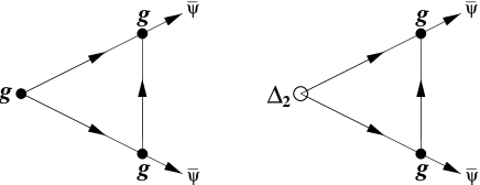
FIG. 5.: One-loop diagrams for the nonlinear vertex $g$ (left) and the Poissonian contribution $\Delta_{2}$ (right). The diagrams are formally equivalent. The same applies to higher loop diagrams that are linear in $\Delta_{2}$ and the corresponding vertex diagrams (not shown here). Hence the loop corrections of these quantities are are identical to all orders in $\epsilon$.

Let us first consider the renormalization of $\Delta_{2}$. As already noticed in Ref. [7], the diagrams in Eq. (24) which are linear in $\Delta_{2}$ are formally identical with those for the renormalization of the nonlinear vertex $g$ to all orders in $\epsilon$ (see Fig. 5). This observation plays a crucial role in the present problem: Since the renormalization of the vertex $g$ is given by

$$\frac{dg}{dl}=g\,\left[z-\frac{d}{2}-\frac{3\eta_{\psi}}{2}-\frac{2g^{2}K_{4}}{\lambda^{2}}+\ldots\right]+0(\epsilon^{2})$$ (25)

we may replace the diagrams of the form $\Delta_{2}[-2g^{2}K_{4}/\lambda^{2}+0(\epsilon^{2})]$ in Eq. (24) by the scaling part $\Delta_{2}[z-d/2-3\eta_{\psi}/2]$ of Eq. (25), resulting in

$$\frac{d\Delta_{2}}{dl}\;=\;\Delta_{2}\left(\frac{\eta_{\psi}-\eta_{\phi}}{2}-z\right)+(\Delta_{2})^{2}\Bigl{[}-\frac{5g^{2}K_{4}}{\lambda^{2}}+0(\epsilon)\Bigr{]}\,.$$ (26)

The linear part of this equation is now exact to all orders in $\epsilon$. Since

$$\frac{\eta_{\psi}-\eta_{\phi}}{2}-z=d_{\psi}-d_{\phi}-z\leq d_{\psi}-z<0$$ (27)

we arrive at the conclusion that $\Delta_{2}$ scales to zero for arbitrary initial states in $d<4$ spatial dimensions. Thus Eq. (23) reduces to its scaling part and hence the scaling dimension of $\Delta_{1}$ is given by

$$d_{\Delta_{1}}=-\frac{\eta_{\psi}+\eta_{\phi}}{2}=d-d_{\psi}-d_{\phi}=\sigma-d_{\psi}\,.$$ (28)

Depending on the sign of $d_{\Delta_{1}}$, the loop corrections for the initial particle distribution are relevant for $\sigma>\sigma_{c}$, irrelevant for $\sigma<\sigma_{c}$, and marginal for $\sigma=\sigma_{c}$.

Continuously changing exponents usually appear when we modify a model with a marginal parameter which is invariant under RG transformations. For example, in case of models with infinitely many absorbing states the initial density plays that role [13]. In our case the two-point correlation of the field $\psi(x,t)$ is characterized by $d_{\psi}=d-\sigma$ for $r>r_{c}(t)$ and is left invariant under the coarse-graining RG transformation, where $r_{c}(t)\to\infty$ is a growing spatial scale. In the infinite time limit this scaling crosses over to $d_{\psi}=\beta/\nu_{\perp}$. The marginality of the operator $S_{ipd}$ requires $\sigma-d_{\psi}=0$ and hence in the infinite time limit we arrive at

$$d_{\psi}(t\to\infty)=\sigma_{c}=\beta/\nu_{\perp}$$ (29)

In the regime $\sigma>\sigma_{c}$ the exponent $\kappa$ is related to the scaling dimension $d_{\Delta_{1}}$ as follows. The particle density is expected to vary in the long time limit as

$$\rho(t)\simeq\rho_{0}\,t^{\kappa}\,,$$ (30)

where $\rho_{0}\propto\Delta_{1}$ is the initial particle density. Under rescaling (15) the density $\rho(t)$ [which is essentially the average of $\psi(x,t)$] scales as $\rho(t)\rightarrow b^{-d_{\psi}}\rho(t)$ while the initial density transforms according to $\rho_{0}\rightarrow b^{-d_{\phi}}\rho_{0}$. Thus scaling invariance of Eq. (30) requires that $-d_{\psi}=z\kappa-d_{\phi}$, i.e.,

$$\kappa=\frac{d_{\phi}-d_{\psi}}{z}=\frac{\eta_{\phi}-\eta_{\psi}}{2z}\,.$$ (31)

In the irrelevant regime $\sigma<\sigma_{c}$, however, the initial density $\rho_{0}$ scales to zero under RG transformations which may be interpreted as an initial state with non-interacting active seeds leading to an increase according to Eq. (2). Combining these results we arrive at Eq. (6) which is exact to all orders in $\epsilon$.

V “Natural” correlations in a DP process

It is interesting to compare the artificial initial states of Sect. II with “natural” DP scaling states. Scaling invariance predicts that a critical DP process, starting from a fully occupied lattice, evolves towards a state with correlations

$$C(r)=\langle s_{i}\,s_{i+r}\rangle\sim r^{-\beta/\nu_{\perp}}\,,\qquad\qquad r\ll\xi_{\perp}$$ (32)

i.e., the “natural” correlations of the critical DP are given by $\sigma^{DP}=d-\beta/\nu_{\perp}$. Interestingly, the corresponding exponent $\kappa(\sigma^{DP})$ vanishes. This means that these correlations characterize a situation where the critical DP process is almost stationary. From the field-theoretical point of view this is not surprising since $\kappa$ is determined solely by the scaling dimension of the initial particle distribution. Nevertheless the result is surprising from the physical point of view since the empty intervals in our artificial initial states are uncorrelated whereas such correlations may exist in DP scaling states. It seems that these correlations are rather weak [12] so that states with uncorrelated intervals can be used as an approximation of DP scaling states. This offers an interesting practical application in DP simulations: Instead of starting a critical DP process from random initial conditions and simulating over long transients, one could use the artificial states of Sect. II with $\sigma=\sigma^{DP}$ as an approximation, followed by a short equilibration period to reach the ‘true’ scaling state of DP.

VI Conclusions

In the present work we numerically studied the temporal evolution of a (1+1)-dimensional critical DP process starting from artificially generated correlated initial states. These states approximate a simple fractal set in which uncorrelated empty intervals are distributed by $P(\ell)\sim\ell^{-\alpha}$. It can be shown that such particle distributions are characterized by long-range correlations of the form $\langle s_{i}s_{i+r}\rangle\sim r^{\sigma-1}$ where $\sigma=\alpha-1$.

The construction of such correlated states is a technically difficult task since lattice spacing and finite-size effects strongly influence the quality of the numerical results, especially close to $\alpha\approx 1$ and $\alpha\approx 2$. In order to minimize these errors, we proposed to project an almost perfect fractal set onto the lattice. Using these states as initial conditions we determined the density $\rho(t)$ in a critical DP process by MC simulations. It varies algebraically with an exponent $\kappa$ that depends continuously on $\sigma$. Therefore correlated initial conditions affect the entire temporal evolution of a critical DP process. The numerical estimates for $\kappa(\sigma)$ are in good agreement with theoretical results from a field-theoretical RG calculation (see Fig. 4). Discrepancies for small values of $\sigma$ can be further reduced by increasing the numerical effort.

The RG calculation is valid for arbitrary spatial dimensions $d<4$ and predicts a critical threshold $\sigma_{c}=\beta/\nu_{\perp}$ where $\kappa(\sigma)$ starts to vary linearly between $+\eta$ and $-\beta/\nu_{||}$. Thus our result in Eq. (6) qualitatively reproduces the scenario predicted by Bray et. al. in the context of coarsening processes [6]. The exact prediction the critical threshold $\sigma_{c}$ is possible because of the irrelevance of $\Delta_{2}$ for arbitrary initial conditions which can be proven by using the formal equivalence of the loop expansions in $g$ and $\Delta_{2}$. It is this property that also allows one to express the critical initial slip exponent $\eta$ by an exact scaling relation $\eta=(\nu_{\perp}-2\beta)/\nu_{||}$. It should be emphasized that some DP models with more complicated dynamical rules violate this scaling relation as, for example, the two-species spreading model discussed in Ref. [7]. In such models the mentioned equivalence of loop expansions in Fig. 5 is no longer valid. Consequently, the corresponding slip exponent $\eta$ takes a different value so that Eq. (6) has to be modified appropriately.

Acknowledgements: We would like to thank M. Howard, K. B. Lauritsen, N. Menyhárd, I. Peschel, and U. C. Täuber for interesting discussions and helpful hints. The simulations were performed partially on the FUJITSU AP-1000 parallel supercomputer. G. Ódor gratefully acknowledges support from the Hungarian research fund OTKA ( Nos. T025286 and T023552) .

REFERENCES

- [1] W. Kinzel, in Percolation Structures and Processes, ed. G. Deutscher, R. Zallen, and J. Adler, Ann. Isr. Phys. Soc. 5 (Adam Hilger, Bristol, 1983), p. 425.
- [2] H. K. Janssen, Z. Phys. B 42, 151 (1981).
- [3] P. Grassberger, Z. Phys. B 47, 365 (1982).
- [4] P. Grassberger and A. de la Torre, Ann. Phys. (N.Y.) 122, 373 (1979).
- [5] H. K. Janssen, B. Schaub, and B. Schmittmann, Z. Phys. B 73, 539 (1989).
- [6] A. J. Bray, K. Humayun, and T. J. Newman, Phys. Rev. B 43, 3699 (1991).
- [7] F. van Wijland, K. Oerding, and H. J. Hilhorst, unpublished (report cond-mat/9706197)
- [8] E. Domany and W. Kinzel, Phys. Rev. Lett. 53, 447 (1984).
- [9] I. Jensen and A. J. Guttmann, J. Phys. A 28, 4813 (1995); I. Jensen, Phys. Rev. Lett.77, 4988 (1996);
- [10] M. Doi, J. Phys. A 9, 1479 (1976); P. Grassberger and P. Scheunert, Fortschr. Phys. 28, 547 (1980); L. Peliti, J. Phys. (Paris) 46, 1469 (1984); B.P. Lee, J. Phys. A 27, 2633 (1994).
- [11] P. Grassberger and K. Sundermeyer, Phys. Lett. 77 B, 220 (1978). J. L. Cardy and R. L. Sugar, J. Phys. A 13, L423 (1980).
- [12] M. Henkel and R. Peschanski, Nucl. Phys. B 390, 637 (1993).
- [13] J. F. F. Mendes, R. Dickman, M. Henkel and Ceu Marques, J. Phys. A: Math. Gen. 27, 3019 (1994).