Critical Behavior of the 4D Spin Glass in Magnetic Field

Abstract

We present numerical simulations of the 4D Edwards Anderson Ising spin glass with binary couplings. Our results, in the midst of strong finite size effects, suggest the existence of a spin glass phase transition. We present a preliminar determination of critical exponents. We discuss spin glass susceptibilities, cumulants of the overlap and energy overlap probability distributions, finite size effects, and the behavior of the disorder dependent and of the integrated probability distribution.

cond-mat/9802224

1 Introduction

The Edwards-Anderson model of spin glasses [1] turns out, not astonishingly, to be hard to be understood. More surprisingly (at the start) also the Sherrington Kirkpatrick mean field version of the model [2] appears to be very complex. Many unprecedented features appear: for example the (spin glass) phase transition survives the presence of a finite magnetic field [3] under the AT line. The Parisi Replica Symmetry Breaking (RSB) solution [4] appears to describe accurately the model in the low $T$ broken phase (and it is believed to be the real solution of the model).

The relevant question is now trying to establish how many of the features of the Parisi solution survive when discussing finite dimensional spin glass models. For example the presence of a phase transition in a finite magnetic field, that is implied by the Parisi solution [4], is not compatible with the point of view of the droplet model [5], where one expects the transition to be removed from the action of a small magnetic field.

As usual in a complex theoretical scenario numerical simulations try to play a role (for a review of recent simulations of spin glass models see [6]). Here we will report numerical simulations that thermalize large lattices with large number of samples: we will try to show many signatures hinting about the presence of a phase transition, and we will be plagued by large finite size effects.

Numerical simulations of spin glasses with non-zero magnetic field have now a long story. Maybe the first work on the subject is the one by Sourlas [7, 8]. The numerical simulations of [9, 10] (see also the criticism in [11] and the reply [12]) use the concept of energy overlap, that turns out to be very relevant in this study: these simulations were giving a first evidence, but the computers of the time allowed too small lattices for getting conclusive results. Simulations of [13] measure constant susceptibility curves [14], and detect the existence of an AT line. On the contrary the work of [15] does not detect one, while [16, 17, 18] are more on the yes side. Again, the work of [19] is negative on the existence of a transition, while [20] claims the difficulty of establishing a firm conclusion (maybe a wise approach). At last recent numerical work using a dynamic approach has been able to claim, again, the existence of a clear transition to a spin glass phase [21, 22].

Here, as we will explain in the next sections, we will find evidence that we consider strongly suggestive of the existence of a phase transition, and we will present very preliminary determinations of critical exponents. We will also find that even on large lattices (on current standards) finite size effects are dramatically strong, and we will discuss them in detail.

2 Numerical Simulations

We will discuss here the $4D$ Edwards-Anderson spin glass system [1] with bimodal quenched random couplings $J=\pm 1$. Our numerical simulations have been using the parallel tempering approach [23], that makes a real difference in the simulations of systems with quenched disorder. The interested reader will find for example in the last of [23] an introduction to optimized Monte Carlo methods (including tempering and, more in general, the multi-canonical approaches).

$L$	Thermalization	Equilibrium	Samples	$N_{\beta}$	$\delta T$	$T_{min}$	$T_{max}$
3	20000	20000	2560	19	0.1	1.0	2.8
5	80000	80000	1920	19	0.1	1.0	2.8
7	200000	200000	960	46	0.04	1.0	2.8
9	150000	150000	64	66	0.04	1.0	3.6

Table 1: Parameters of the tempered Monte Carlo runs.

We report in table (1) the parameters relevant for our tempered simulations: for each lattice size we give the number of discarded thermalization sweeps and of the sweeps used for measurements, the total number of samples that we have analyzed, the number of temperatures used in each tempered run (i.e. the number of copies of the system updated in parallel at different $\beta$ values and among which the temperature values have been swapped), the temperature increment, the minimum and the maximum temperature.

The $\beta$ values have been chosen, as customary and reasonable, in order to keep the acceptance factor of the tempering $\beta$ swap of order $\frac{1}{2}$. In our case we have a $\beta$ acceptance ratio close to $0.8$ for $L=3$ that goes down to a number close to $0.6$ at $L=9$.

Our runs are surely well thermalized for $L\leq 7$: for each copy $\beta$ has visited all possible values at least a few times, and the system has never been stuck. $L=9$ is more delicate, and we are not sure that the data points with lower $T$ values are fully thermalized: we have repeated different trial runs, with different values of the parameters, and the one we report here are the ones that turn out to be better thermalized. Difference among the different runs were in any case minor, and a possible remanence of on thermalization effects would affect only minor issues that we will point out in the following. Here we will only insist on features that are surely representing thermal equilibrium even on the $L=9$ lattice.

3 Spin Glass Susceptibilities

In this section we will discuss the overlap and the energy overlap susceptibilities. We will show the signature of a spin glass like phase transition. We will discuss the location of the critical temperature and the determination of the critical exponents.

We consider two real replicas of the system with spins $\sigma_{i}$ and $\tau_{i}$, and the local energy operator

$$\epsilon_{i}^{(\sigma)}\equiv\frac{1}{2D}\sigma_{i}\sum_{j}J_{i,j}\sigma_{j}\ ,$$ (1)

where the sum runs over first neighbors of the site $i$ (on a $4D$ hypercubic lattice of linear size $L$ and volume $V=L^{4}$). The overlap operator is defined as

$$q\equiv\frac{1}{V}\sum_{i}\sigma_{i}\tau_{i}\ ,$$ (2)

and the energy overlap operator as

$$q_{E}\equiv\frac{1}{V}\sum_{i}\epsilon^{(\sigma)}_{i}\epsilon^{(\tau)}_{i}\ .$$ (3)

This operator plays a crucial role, since it allows to distinguish a possible trivial replica symmetry breaking from a non-trivial breaking. In the Mean Field RSB $q_{E}$ and $q^{2}$ coincide, while a non-trivial behavior of $q$ induced by the presence of interfaces would generate a trivial $q_{E}$. Detecting a non-trivial behavior of $q_{E}$ is strong evidence for a RSB like behavior. We will consider the probability distribution of the overlap for a given sample of the quenched disorder, $P_{J}(q)$, and the same for the energy overlap, $P^{E}_{J}(q)$. We will call $P(q)$ and $P^{E}(q)$ the probability distribution integrated over the quenched disorder.

We define the overlap susceptibility as

$$\chi_{q}\equiv V\left(E(q^{2})-E(q)^{2}\right)\ ,$$ (4)

where by $E(\ \cdot\ )$ we denote the combined operation of a thermal average and an average over the quenched disorder $J$ (in the usual notation $E(\ \cdot\ )=\overline{\langle\ \cdot\ \rangle}$). We define the energy overlap susceptibility as

Figure 1: $\chi$ as a function of $T$. Empty squares for $L=9$, asterisks for $L=7$, crosses for $L=5$ and horizontal bars for $L=3$.

$$\chi_{q_{E}}\equiv V\left(E(q_{E}^{2})-E(q_{E})^{2}\right)\ .$$ (5)

In figure (1) we plot the overlap susceptibility $\chi$ as a function of $T$ for $L=3$, $5$, $7$ and $9$, and in figure (2) we plot the energy overlap susceptibility $\chi_{E}$. The statistical errors are computed using a jack-knife algorithm.

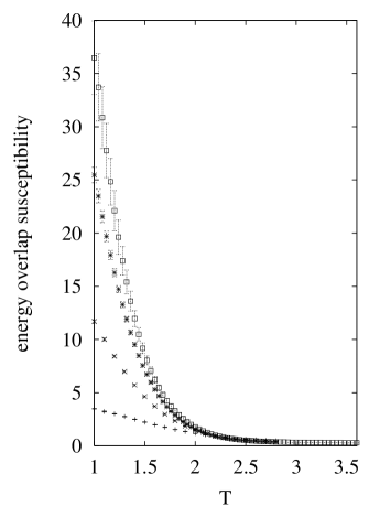
Figure 2: As in figure (1) but for $\chi_{q_{E}}$.

Both susceptibilities show a divergence in the low $T$ region. The comparison of figure (1) with the analogous plot of reference [20] shows a difference: we do not see a cusp but a clear divergence (not only for $L=7$ but also for $L=9$ down to $T=1.0$). We believe this is very well explained from some non complete thermalization for the larger lattices of reference [20] (this possibility is proposed and discussed in reference [20] itself: a non complete thermalization has exactly the effect of smoothing the divergence, since correlations on large scale cannot be created): these measurements are very delicate. As we have already discussed we are completely safe as far as the $L=7$ lattice is concerned, but $L=9$ was clearly our limit. It is important to stress that this is the only point of discrepancy with reference [20]: as far as other (less sensitive) quantities are concerned (and even for the susceptibility on the two smaller lattice sizes) we find exactly the same results. Reference [20] does not analyze the quantities based on the energy overlap.

As we have said the divergence of the two susceptibilities is clear. We are able to follow the divergence on thermalized lattices down to $T=1.0$. The fact that also the energy overlap susceptibility diverges makes a stronger case for a RSB like spin glass phase. The analysis of reference [21] hints that at $h=0.4$ is close or slightly lower than $1.5$. We just note at this point that the data of figures (1) and (2) are fully compatible with this value.

Figure 3: $\log(\chi_{q})$ and best fit to a power law (continuous line) and $\log(\chi_{q_{E}})$ and best fit to a power law (dashed line) versus the logarithm of the reduced temperature.

One can see in figures (1) and (2) that there is a temperature region where the behavior is asymptotic (i.e. measurements on the $L=9$ lattice are compatible with the ones taken on smaller lattices). We use this region to fit the susceptibility as a function of the reduced temperature $\frac{T}{T-T_{c}}$, with

$$\chi_{q}(t) \simeq A_{q}t^{-\gamma}\ ,$$

$$\chi_{q_{E}}(t) \simeq A_{q_{E}}t^{-\gamma_{\epsilon}}\ .$$ (6)

We will use the value $T_{c}=1.4$ (in agreement with the results of [21] and with evidence that will be discussed later in this note). The fits in the region of $T$ going from $2.1$ to $2.6$ (that we show in figure (3)) give $\gamma=1.97$ and $\gamma_{\epsilon}=1.93$. $\chi_{q}$ has a stronger $L$ dependence than $\chi_{q_{E}}$. We plot in figure (3) the logarithm of $\chi_{q}$ and $\chi_{q_{E}}$ versus $\log(t)$, and the best fits to the form (6).

The conclusion of this analysis is that the numerical data are compatible with a divergence at $T_{c}\simeq 1.4$ with an exponents $\gamma$ and $\gamma_{\epsilon}$ close to $2$.

We have also carried through a standard finite size scaling analysis, by selecting $T_{c}$ and the critical exponents in such a way to have curves at different lattice size collapsing together as well as possible. As usual for not very accurate data (as is unfortunately frequently the case for numerical simulations of complex systems) this analysis does not give unambiguous results, but only hints reasonable and preferred set of values. We use for $\chi_{q}$ the leading scaling form

$$\chi_{q}=L^{\frac{\gamma}{\nu}}\overline{\chi}_{q}\left(L^{\frac{1}{\nu}}(T-T_{c})\right)\ ,$$ (7)

and the same form for $\chi_{q_{E}}$. By looking at $\chi_{q}$ we find that $T_{c}=1.4$, $\frac{1}{\nu}=0.7$ and $\frac{\gamma}{\nu}=1.3$ give a very good fit. The same values (with $\gamma_{\epsilon}=\gamma$) also give a very good scaling behavior for $\chi_{q_{E}}$.

If one would take a higher value of $T_{c}$ (that could be suggested by a possible interpretation of the crossover regime we will discuss in the next section, but is discouraged by the dynamical data of [21]), for example $T_{c}=1.8$, we would find a higher value of $\nu$, of the order of two, and $\frac{\gamma}{\nu}\simeq 1$. Again, the finite size scaling analysis and the study of the asymptotic $T$ dependence would be consistent at this effect.

4 Skewness and Kurtosis

In order to qualify the probability distribution of the overlap and of the energy overlap we will define and analyze their kurtosis (the Binder cumulant) and their skewness. For zero-field deterministic and disordered statistical systems the Binder cumulant $g$ of the order parameter is a very good signature of the phase transition: curves of $g$ versus $T$ cross at the critical point, since the kurtosis of the probability distribution of the order parameter at the critical point is an universal quantity. In the infinite volume limit $g$ goes to zero in the warm phase: it goes to one in a ferromagnetic phase, and to a non-trivial function in the broken phase of the Parisi RSB solution of the mean field spin glass theory.

Here, since we have a non zero magnetic field, we have to consider connected expectation values. We define the overlap kurtosis on a lattice of linear size $L$ as

$$g(T)\equiv\frac{3}{2}-\frac{1}{2}\frac{E\left(\left(q-E(q)\right)^{4}\right)}{E\left(\left(q-E(q)\right)^{2}\right)^{2}}\equiv\frac{3}{2}-\frac{1}{2}\frac{\chi_{q}^{(2)}}{\chi_{q}^{2}}\ ,$$ (8)

which defines $\chi^{(2)}_{q}$. We define the kurtosis for the energy overlap $g_{\epsilon}$ in the analogous way, by using $q_{E}$. We define the skewness of the probability distribution of the overlap as

$$s(T)\equiv\frac{E\left(\left(q-E(q)\right)^{3}\right)}{E\left(\left(q-E(q)\right)^{2}\right)^{\frac{3}{2}}}\equiv\frac{\chi_{q}^{(\frac{3}{2})}}{\chi_{q}^{\frac{3}{2}}}\ ,$$ (9)

which defines $\chi^{(\frac{3}{2})}_{q}$. In the definition of the skewness of the energy overlap probability distribution $s_{\epsilon}$ one substitutes $q_{E}$ to $q$. We note now that the study of the $q_{E}$ probability distribution turns out to be very important. We plot $g(T)$ for the four different lattice volumes in figure (4). In this and in next plots errors are from sample-to-sample fluctuations evaluated with a jack-knife analysis.

Figure 4: As in figure (1) but for the overlap kurtosis $g$.

The difference with the usual zero field picture is strong. There is a clear change of regime close to $T=2$ (the critical point at $h=0$). The $L=3$ system is small and different, and never really gaussian in our $T$ range. For $L\geq 5$ $g$ becomes non-trivial when $T$ becomes smaller than $2$. The $q$-kurtosis in this region does not change much with size. In the statistical error the values of the $L=5$, $7$ and $9$ lattice are compatible (but maybe at $T\simeq 1$ where also small non-equilibrium effects have to be accounted for). The fact that the kurtosis does not depend on $L$ and is non-trivial is very clear from our data. Again, the traditional crossing behavior is completely absent (likely even in the infinite volume limit) in our data. Two things must be stressed here: first of all that the existence or non-existence of a crossing also depends from the shape of the critical asymptotic probability distribution, and second that we cannot exclude, and on the contrary we clearly detect (see for example next figure, (5)) the existence of very strong finite size effects.

Figure 5: As in figure (1) but for the energy overlap kurtosis $g_{\epsilon}$.

Figure (5), where we plot the energy overlap kurtosis, is dramatically and delightfully different from figure (4). It is already very interesting to look at the high $T$ region: here only the $L=9$ lattice starts to be gaussian, while smaller lattices have a strongly non-gaussian behavior. In the cold region again there is a strong finite size dependence (we will see in the next section that there is a finite size double peak structure that is disappearing on large lattices). Here there is a crossing, even if it is inverted as compared to usual, $h=0$ systems, where in the warm phase the kurtosis curves become lower with increasing lattice size: in our case for small sizes and high $T$ we have a negative kurtosis, that tends to zero from below when the size increases. This real, inverted crossing is at $T$ higher than $1.5$, but we believe it should be taken cum grano salis as far as the exact determination of the critical point is concerned. The finite size effects make themselves clear in the non-gaussian behavior in the warm phase, and in a peak in the cold phase, that shrinks and shifts with increasing lattice size (see figure (5)). A value of $T_{c}\simeq 1.5$ is very compatible with this picture.

Figure 6: As in figure (1) but for the overlap skewness $s$.

The behavior of the skewness for the overlap (6) and for the energy overlap (7) repeats a similar pattern. We find a symmetric behavior of the overlap in the warm phase, and curves collapse to a non-trivial shape in the low $T$ regime. The energy overlap skewness, on the contrary, starts to become zero in the warm region only on our larger lattice, $L=9$, and heavily depends on $L$ in the low $T$ region. Again a peak close to $T\simeq 2$ is shrinking with increasing lattice size.

Figure 7: As in figure (1) but for the energy overlap skewness $s_{\epsilon}$.

In the next section we will discuss the full probability distribution. The analysis we have discussed here strongly suggests the existence of a RSB phase. We have been able to get hints for the value of $T_{c}$ and of the critical exponents, but such estimates, that surely improve on existing ones, have to be considered only as hints.

5 Probability Distributions

Before starting a detailed discussion of the behavior of the probability distribution of the order parameter for a given sample $P_{J}(q)$ and of the disorder averaged $P(q)$ we briefly discuss finite size effects on, for example, $\langle q\rangle_{L}$. We have analyzed the size dependence of $\langle q\rangle_{L}$ and $\langle q_{E}\rangle_{L}$. We have tried a fit of the type (see [17] for a detailed discussion of the issue)

$$\langle q\rangle_{L} \simeq \langle q\rangle_{\infty}+\frac{A}{L^{d_{q}}}\ ,$$

$$\langle q_{E}\rangle_{L} \simeq \langle q_{E}\rangle_{\infty}+\frac{A_{E}}{L^{d_{q_{E}}}}\ .$$ (10)

In the Parisi solution of the mean field theory $d_{q}=d_{q_{E}}$: corrections that scale as $V^{-\frac{1}{3}}$ and the fact that the upper critical dimension is $6$ imply that in the mean field limit we expect $d_{q}=2$.

We find that for the overlap the best fit to $d_{q}$ (using $L=3$, $5$, $7$ and $9$) increases with $T$ from $2.3\pm 0.5$ at $T=1.0$ to $3.2\pm 0.2$ at $T=1.6$, and to a number larger than $4$ for $T$ among $2$ and $3$ (for $T>T_{c}$ we expect an exponential decay, but on a finite lattice with a finite number of points we can fit an effective exponent). $d_{q_{E}}$ is larger: here finite size effects are smaller, and the exponent more difficult to determine. In the region of $T=1.6$, $1.8$, $2.0$ we find an exponent close to $4$, that increases in the high $T$ region. For example at $T=1.6$, that asymptotically is probably marginally off-critical but very close to the estimated $T_{c}$, where we have a clean determination of both exponents, we have a ratio $\frac{d_{q_{E}}}{d_{q}}\simeq\frac{4}{3}$ (to be compared with the $1$ that one finds in the mean field theory). The behavior of $\langle q\rangle_{L}$ does not look compatible with a pure exponential, while $\langle q_{E}\rangle_{L}$ would also be compatible with an exponential decay. We stress again that since the expected finite size corrections have a very complex pattern (different terms could be leading for different $L$ values) the exact theoretical significance of this numerical result is not clear (see [17] for a discussion), but for the fact that we find that the two exponents are not very different from the ones that are found in mean field. For a comparison of the equilibrium value $E(q)$, and the dynamical value of the overlap, $q_{D}$, see figure two of ref. [21] (our data for $E(q)$ are very similar to the ones of [20]).

Figure 8: $P(q)$ at $L=9$ for different $T$ values: from the left are the curves for $T=2.4$, $2.2$, $2.0$, $1.6$, $1.4$, $1.2$, $1.0$.

Let us examine in some more detail now the full $P(q)$ and $P^{E}(q)$ and the probability distributions for a given sample, $P_{J}(q)$ and $P^{E}_{J}(q)$. In figure (8) we plot $P(q)$ at $L=9$ for different $T$ values. At $T=2.4$ $P$ is gaussian and symmetric. For lower $T$ values we get a strong deviation from a Gaussian behavior. We will discuss later the fact that finite volume effects are very strong (and they turn out to be the most serious limitation in the case of the simulations we are discussing here). We can already notice that at $T=1$ from the results of [21] we expect that the minimum value allowed for the overlap is $q_{min}\simeq 0.55$. On the contrary even on our larger size, $L=9$, we get a long tail that basically goes down to $q=0$ (we will see later that it goes down to $-1$ for the smaller lattice sizes).

Figure 9: As in figure (8) but for $P^{E}(q)$.

A very similar pattern holds for $P^{E}(q)$ in figure (9). Here even at $L=9$ and at $T=2.4$ (deep in the warm phase) the probability distribution is not yet fully gaussian (as one can also see from the kurtosis and the skewness). As for $P(q)$ the distribution becomes very asymmetric at low $T$, with a large tail towards small overlaps.

Figure 10: $P(q)$ versus $q$ at $T=2.0$ for $L=3$, $5$, $7$ and $9$ (curves from bottom to top).

It is interesting to analyze in more detail the size dependence of the probability distributions. In figure (10) we show $P(q)$ versus $q$ at $T=2.0$ for $L=3$, $5$, $7$ and $9$. This is the point of the transition in the $h=0$ model, asymptotically in the warm region for $h=0.4$. Clearly for $L=3$ the distribution is far from Gaussian: only at $L=7$ one sees a Gaussian behavior.

Figure 11: As in figure (10) but $T=1.0$.

The same function at low $T$ is very different. We show $P(q)$ versus $q$ at $T=1.0$ in figure (11). Also here finite size effects are very large, but $P(q)$ does not show any sign of convergence to a gaussian behavior. In the mean field RSB solution one would expect a delta function at $q_{min}$ (that, as we already said, at $T=1.0$ is close to $0.55$ [21]): here, at least for $L<9$, we do not see a $\delta$ function like contribution at $q<q_{max}$. Only at $L=9$ we see a small bump at $q\simeq 0.2$: we see it in all our different runs, but we cannot exclude (and on the contrary we believe it is possible) that it is due to lack of complete thermalization of the $L=9$ data at the lower $T$ values (as we have discussed even if quantities like $\langle q^{2}\rangle$ are well behaved and apparently thermalized we cannot completely exclude a very small effect of this kind). Also we will discuss a similar effect, that turns out to be due to the finite size of the lattice, for the energy overlap.

Figure 12: As in figure (10) but $P_{E}$.

In figure (12) we show $P_{E}(q_{E})$ versus $q$ at $T=2.0$ for $L=3$, $5$, $7$ and $9$. Again, on small lattices even at warm $T$ $P_{E}$ is not symmetric (the tail is in this case for large values of the overlap).

Figure 13: As in figure (10) but $P_{E}$ and $T=1.0$.

In figure (13) we show that in the cold region ($T=1$) the energy overlap has even stronger finite size effects than the spin-spin overlap. Here a spurious peak at low values of $q_{E}$ is very strong for small $L$ values (it carries the thirty percent of the weight at $L=3$), and becomes smaller and smaller on larger lattices.

Figure 14: A first $P_{J}(q)$ for one disorder sample, $L=9$ and $T=1$.

We also show, in figures (14) and (15) two individual $P(q)$ for two different realizations of the quenched disorder at $L=9$, $T=1$. It is clear that different samples can have a very different equilibrium probability distribution, and the system does not look self-averaging. In the two examples we show, for example, it is clear that, like in mean field theory, we can find systems with one maximum of $P(q)$ and systems with a complex structure of $P(q)$, with many local maxima. The integrated $P(q)$ is not originated from a trivial sum of very similar individual $P_{J}(q)$, but from the sum of individual very different distributions. It is clear that this feature, crucial in the RSB mean field picture, is shared by the finite dimensional system in a non-zero magnetic field.

Figure 15: A second $P_{J}(q)$ for a different disorder sample, $L=9$ and $T=1$.

6 Conclusions

We have discussed accurate numerical simulations of the 4D Edwards Anderson spin glass in magnetic field. Our results hint very strongly the existence of a spin glass phase transition. Susceptibilities grow strongly at low $T$, and fits to a divergent behavior are very good. Cumulants of the overlap and energy overlap probability distribution like the kurtosis and the skewness show a clear change of regime in the region of temperatures lower than the $h=0$ critical point. Finite size effects are dominated by power laws that are similar to the ones of the mean field theory. Probability distributions are non-trivial in the low $T$ region, and, what is most important, different samples behave clearly in very different ways. The energy overlap follows the usual overlap in this RSB like behavior, making the possibility of a non-trivial behavior caused by interfaces quite unplausible.

There are also differences with the usual RSB like picture at $h=0$. For example here the Binder cumulants do not cross (and the pictures of the $P(q)$ show why). What is more impressive and relevant is the presence of very strong finite size effects (even on lattices of size $L^{4}=9^{4}$, that had never before been thermalized in a numerical simulation). These effects are far larger than in the $h=0$ case. This is the most important limitations of the present numerical simulation (and of the physics conclusions one can draw from them): when finite size effects are as strong as we have shown is very difficult to be sure that any asymptotic behavior has been observed. Because of that all the quantitative results we quote for critical exponents and temperatures have to be taken as simple indications. The other real problem, as far as the coincidence with the RSB mean field picture is concerned, is that even for $L=9$ we do not see any trace of a $\delta$-function at $q=q_{min}$: even if on theoretical grounds we expect this peak to be smaller than the one at $q_{max}$ [17], and if we know that finite size effects are very strong, and if we have a small bump in $P(q)$ at $L=9$ at low $q$ (that we cannot take too seriously), this a worrying point, that is there to demand further clarification.

References

- [1] S. F. Edwards and P. W. Anderson, Theory of Spin Glasses, J. Phys. F: Metal Phys. 5, 965 (1975).
- [2] D. Sherrington and S. Kirkpatrick, Solvable Model of a Spin-Glass, Phys. Rev. Lett. 35, 1793 (1975); S. Kirkpatrick and D. Sherrington, Infinite-Ranged Models of Spin-Glasses, Phys. Rev. B 17, 4384 (1978).
- [3] J. R. L. de Almeida and D. J. Thouless, Stability of the Sherrington-Kirkpatrick Solution of a Spin Glass Model, J. Phys. A: Math. Gen. 11, 983 (1978).
- [4] G. Parisi, Phys. Lett. 73A, 203 (1979); Phys. Rev. Lett. 43, 1754 (1979); J. Phys. A: Math. Gen. 13, L115 (1980); 1101; 1887; Phys. Rev. Lett. 50, 1946 (1983).
- [5] W. L. McMillan, J Phys. C 17, 3179 (1984); D. S. Fisher and D. A. Huse, Phys. Rev. Lett. 56, 1601 (1986); Phys. Rev. B 38, 386 (1988); A. J. Bray and M. A. Moore, in Glassy Dynamics and Optimization, edited by J. L. van Hemmen and I. Morgenstern (Springer, Berlin 1986)
- [6] E. Marinari, G. Parisi and J. J. Ruiz-Lorenzo, Numerical Simulations of Spin Glass Systems, in Spin Glasses and Random Fields, edited by P. Young (World Scientific, Singapore 1997), cond-mat/9701016.
- [7] N. Sourlas, Dynamical Behavior of Three-Dimensional Ising Spin Glass, Europhys. Lett. 1, 189 (1986).
- [8] N. Sourlas, Three-Dimensional Ising Spin Glasses and Ergodicity Breaking, Europhys. Lett. 6, 561 (1988).
- [9] S. Caracciolo, G. Parisi, S. Patarnello and N. Sourlas, Ising Spin Glasses in a Magnetic Field and Mean Field Theory, Europhys. Lett. 11, 783 (1990).
- [10] S. Caracciolo, G. Parisi, S. Patarnello and N. Sourlas, Low Temperature Behavior of 3-D Spin Glasses in a Magnetic Field, J. Phys. France 51, 1877 (1990).
- [11] D. A. Huse and D. S. Fisher, On the Behavior of Ising Spin Glasses in a Uniform Magnetic Field, J. Phys. I France 1, 621 (1991).
- [12] S. Caracciolo, G. Parisi, S. Patarnello and N. Sourlas, On Computer Simulations for Spin Glasses to Test Mean Field Predictions, J. Phys. I France 1, 627 (1991).
- [13] E. R. Grannan and R. E. Hetzel, Susceptibility of Two-, Three-, and Four-Dimensional Spin Glasses in a Magnetic Field, Phys. Rev. Lett. 67, 907 (1991).
- [14] R. R. P. Singh and D. A. Huse, J. Appl. Phys. 69, 5225 (1991).
- [15] N. Kawashima and N. Ito, Critical Behavior of the Three-Dimensional Model in a Magnetic Field, J. of the Phys. Soc. of Jap..
- [16] D. Badoni, J. C. Ciria, G. Parisi, J. Pech, F. Ritort and J. J. Ruiz-Lorenzo, Europhys. Lett. 21, 495 (1993).
- [17] J. C. Ciria, G. Parisi, F. Ritort and J. J. Ruiz-Lorenzo, The de Almeida-Thouless Line in the Four Dimensional Ising Spin Glass, J. Phys. I France 3, 2207 (1993).
- [18] M. Picco and F. Ritort, Numerical Study of the Ising Spin Glass in a Magnetic Field, J. Phys. I France 4, 1619 (1994).
- [19] J. O. Andersson, J. Mattsson and P. Svedlindh, Phys. Rev. B 49, 1120 (1994).
- [20] M. Picco and F. Ritort, Tempering Simulations on the Four Dimensional Ising Spin Glass in a Magnetic Field, cond-mat/9702041 (February 1997).
- [21] E. Marinari, G. Parisi and F. Zuliani, 4D Spin Glasses in Magnetic Field Have a Mean Field Like Phase, J. Phys. A, to be published, cond-mat/9703253 (March 1997).
- [22] G. Parisi, F. Ricci-Tersenghi and J. J. Ruiz-Lorenzo, On the Dynamics of the 4d Spin Glass in a Magnetic Field, cond-mat/9711122 (November 1997).
- [23] E. Marinari and G. Parisi, Europhys. Lett. 19, 451 (1992); M. C. Tesi, E. Janse van Rensburg, E. Orlandini and S. G. Whillington, J. Stat. Phys.; K. Hukushima and K. Nemoto, J. Phys. Soc. Japan 65, 1604 (1996); E. Marinari, Optimized Monte Carlo Methods, lectures given at the 1996 Budapest Summer School on Monte Carlo Methods, ed. by J. Kertesz and I. Kondor, Springer-Verlag, to be published, cond-mat/9612010.