[

3D Spinodal Decomposition in the Inertial Regime

Abstract

We simulate late-stage coarsening of a 3D symmetric binary fluid using a lattice Boltzmann method. With reduced lengths and times, $l$ and $t$ respectively (with scales set by viscosity, density and surface tension) our data sets cover $1\ \raisebox{-0.86108pt}{$\stackrel{{\scriptstyle\scriptstyle<}}{{\scriptstyle\sim}}$}\ l\ \raisebox{-0.86108pt}{$\stackrel{{\scriptstyle\scriptstyle<}}{{\scriptstyle\sim}}$}\ 10^{5}$, $10\ \raisebox{-0.86108pt}{$\stackrel{{\scriptstyle\scriptstyle<}}{{\scriptstyle\sim}}$}\ t\ \raisebox{-0.86108pt}{$\stackrel{{\scriptstyle\scriptstyle<}}{{\scriptstyle\sim}}$}\ 10^{8}$. We achieve Reynolds numbers approaching $350$. At Re $\ \raisebox{-0.86108pt}{$\stackrel{{\scriptstyle\scriptstyle>}}{{\scriptstyle\sim}}$}\ 100$ we find clear evidence of Furukawa’s inertial scaling ($l\sim t^{2/3}$), although the crossover from the viscous regime ($l\sim t$) is very broad. Though it cannot be ruled out, we find no indication that Re is self-limiting ($l\sim t^{1/2}$) as proposed by M. Grant and K. R. Elder$\left[\right.$Phys. Rev. Lett. 82, 14 (1999)$\left.\right]$.  

(Received 25 February 1999)

PACS numbers: 64.75+g, 07.05.Tp, 82.20.Wt

] When an incompressible binary fluid mixture is quenched far below its spinodal temperature, it will phase separate into domains of different composition. Here we consider only fully symmetric 50/50 mixtures in three dimensions, for which these domains will, at late times, form a bicontinuous structure, with sharp, well-developed interfaces. The late-time evolution of this structure remains incompletely understood despite theoretical [1, 2, 3, 4], experimental [5] and simulation [6, 7, 8, 9, 10] work.

As emphasized by Siggia [1] and Furukawa [2], the physics of spinodal decomposition involves capillary forces, viscous dissipation, and fluid inertia. Thus, assuming that no other physics enters, the control parameters are interfacial tension $\sigma$, fluid mass density $\rho$, and shear viscosity $\eta$. From these can be constructed only one length, $L_{0}=\eta^{2}/\rho\sigma$ and one time $T_{0}=\eta^{3}/\rho\sigma^{2}$. We define the lengthscale $L(T)$ of the domain structure at time $T$ via the structure factor $S(k)$ as $L=2\pi\int S(k)dk/\int kS(k)dk$. The exclusion of other physics in late stage growth then leads us to the dynamical scaling hypothesis [1, 2]: $l=l(t)$, where we use reduced time and length variables, $l\equiv L/L_{0}$ and $t\equiv(T-T_{int})/T_{0}$. Since dynamical scaling should hold only after interfaces have become sharp, and transport by molecular diffusion ignorable, we have allowed for a nonuniversal offset $T_{int}$; thereafter the scaling function $l(t)$ should approach a universal form, the same for all (fully symmetric, deep-quenched, incompressible) binary fluid mixtures.

It was argued further by Furukawa [2] that, for small enough $t$, fluid inertia is negligible compared to viscosity, whereas for large enough $t$ the reverse is true. Dimensional analysis then requires the following asymptotes:

$$l\to bt\mbox{;\hskip 30.00005pt}t\ll t^{*}$$ (1)

$$l\to ct^{2/3}\mbox{;\hskip 30.00005pt}t\gg t^{*}$$ (2)

where, if dynamical scaling holds, amplitudes $b,c$ (and the crossover time $t^{*}$) are universal. The Reynolds number, conventionally defined as, ${\mathrm{R}e}=\rho/\eta LdL/dT=l\dot{l}$, becomes indefinitely large in the inertial regime, Eq. (2).

In a recent paper, Grant and Elder have argued [4] that the Reynolds number cannot, in fact, continue to grow indefinitely. If so, Eq. (2) is not truly the large $t$ asymptote, which must instead have $l\sim t^{\alpha}$ with $\alpha\leq\frac{1}{2}$. Grant and Elder argue that at large enough Re, turbulent remixing of the interface will limit the coarsening rate [4], so that Re stays bounded. A saturating Re (which they estimate as Re $\sim 10-100$) would require any $t^{2/3}$ regime to eventually cross over to a limiting $t^{1/2}$ law. But if a single length scale $l\sim t^{1/2}$ is involved, a saturating Re implies balance between viscous and inertial terms ($t^{-3/2}$), while the driving term (interfacial tension) remains much larger than either ($t^{-1}$). This suggests a failure of scaling altogether, with at least two length scales relevant at late times. In any case, the arguments of Grant and Elder are far from rigorous; the coarsening interfaces could, remain one step ahead of the remixing despite an ever-increasing Re which, if applied to a static interfacial structure, would break it up. Thus Eq. (2) cannot yet be ruled out as a limiting law.

In what follows we present the first large-scale simulations of 3D spinodal decomposition to unambiguously attain a regime in which inertial forces dominate over viscous ones. We find direct evidence for Furukawa’s $l\sim t^{2/3}$ scaling, Eq. (2). Although a further crossover to a regime of saturating Re cannot be ruled out, we find no evidence for this up to Re $\simeq 350$. Our work, which is of unprecedented scope, also probes the viscous scaling regime $[$Eq. (1)$]$, and the nature of the crossover between this and Eq. (2). Full details of our results [11] and of the simulation algorithm [12] will be published elsewhere.

Our simulations use a lattice Boltzmann (LB) method [13, 14] with the following model free energy:

$$F=\int d{\mathbf{r}}\left\{-\frac{A}{2}\phi^{2}+\frac{B}{4}\phi^{4}+\tilde{\rho}\ln\tilde{\rho}+\frac{\kappa}{2}|\nabla\phi|^{2}\right\},$$ (3)

in which $A$, $B$ and $\kappa$ are parameters that determine quench-depth (${A/B}\to 1$ for a deep quench) and interfacial tension ($\sigma=\sqrt{8\kappa A^{3}/9B^{2}}$); $\phi$ is the usual order parameter (the normalized difference in number density of the two fluid species); $\tilde{\rho}$ is the total fluid density, which remains (virtually) constant throughout [14, 15].

The simulation code follows closely that of [14] (for details see [11, 12]) and uses a cubic lattice with nearest and next-nearest neighbor interactions (D3Q15). It was run on Cray T3D and Hitachi SR-2201 parallel machines with system sizes up to $256^{3}$. The LB method allows the user to choose $\eta,\sigma,\rho$ (we set $\rho=1$ without loss of generality), along with the order-parameter mobility $M$ defined via $\dot{\phi}=\nabla\cdot M\nabla(\delta F/\delta\phi)$. Although it plays no role in the arguments leading to Eqs. (1) and (2), $M$ must be chosen with some care to ensure that at late times (a) the algorithm remains stable, (b) the local interfacial profiles remain close to equilibrium (so that $\sigma$ is well-defined), and (c) the direct contribution of diffusion to coarsening is negligibly small. Table I shows the parameters used for our eight $256^{3}$ runs.

TABLE I.: Parameters used in LB runs

$L_{0}$		$T_{0}$			A,B		$\kappa$		$\eta$		M		$\sigma$
36		930		0	.083	0	.053	1	.41	0	.1	0	.055
5	.9	71		0	.0625	0	.04	0	.5	0	.5	0	.042
5	.9	71		0	.0625	0	.04	0	.5	0	.2	0	.042
0	.95	4	.5	0	.0625	0	.04	0	.2	0	.3	0	.042
0	.15	0	.89	0	.00625	0	.004	0	.025	4	.0	0	.0042
0	.010	0	.016	0	.00625	0	.004	0	.0065	2	.5	0	.0042
0	.00095	0	.00064	0	.00313	0	.002	0	.0014	8	.0	0	.0021
0	.00030	0	.00019	0	.00125	0	.0008	0	.0005	10	.0	0	.00082

In all runs, the interface width is $\xi\simeq 5\sqrt{\kappa/2A}\simeq 3$ in lattice units. This was found [11] to be the minimum acceptable to obtain an accurately isotropic surface tension. To minimise diffusive effects, data for which the diffusive contribution to the growth rate was greater than 2% was discarded [16]; this corresponded to a minimum value of $L$ of $15<L_{min}<24$, depending on the run parameters. The large size of our runs allowed a ruthless attitude to finite size effects: we use no data with $L>\Lambda/4$, with $\Lambda$ the linear system size. In our $256^{3}$ runs, these filters mean that the good data from any single run lies within $20\ \raisebox{-0.86108pt}{$\stackrel{{\scriptstyle\scriptstyle<}}{{\scriptstyle\sim}}$}\ L\leq 64$, a comparable range to previous studies [6, 7, 8]. Datasets of high and low $L_{0}$ are well fit respectively by $\alpha=1$ and $\alpha=2/3$ (see Fig.1).

FIG. 1.: $L$ vs. $T$ for the runs shown in Table I with $L_{0}$ = 5.9 (M = 0.2) (circles) and 0.0003 (diamonds). The region used for fitting is delimited by ($L_{min}<L<L_{max}=64$) and the fits are projected back to show the intercepts, $T_{int}$. The fits (solid) are to $\alpha=1,2/3$; free exponent fits are also shown (dashed), with best fit values $\alpha=1.16,0.69$.

However, as emphasized by Jury et al. [8], meaningful tests of scaling are best made not by looking at single data sets but by combining those of different parameter values. To this end, the good data from each run were fit to $L=B(T-T_{int})^{\alpha}$, so as to extract an intercept $T_{int}$; we then transformed the data to reduced physical units $l$ and $t$ defined above. The exponent $\alpha$ was first allowed to float freely; this gave reproducible values at large $l$ and $t$ (e.g., $\alpha=0.69$ and $0.67$ for the last two data sets in Table 1), but more scattered ones at small $l$ and $t$ ($\alpha=0.88$, $0.86$ and $1.16$ for the first three data sets). In the latter region the floating fit is relatively poorly conditioned; it also gives large relative errors in $T_{int}$ (see Fig.1). In contrast, fits to $\alpha=1$ for these three data sets gave much better data collapse with consistent values of $b$ ($b=0.073$, $0.073$ and $0.072\pm 0.01$). Thus we are confident of $\alpha=1$ in this region. For the remaining data sets we estimate errors in individual exponent values at around 10% and in reduced time $t$ around 3% to 10%. Figure 2 shows all our data sets on a single plot using reduced variables $l$ and $t$. Such a plot is necessarily log-log, since our data sets span seven decades in $t$ and five in $l$, a range which exceeds all previous studies combined.

FIG. 2.: Scaling plot in reduced variables $(l,t)$ for LB data, bold lines (left to right) are those of Table I (top to bottom). Squares Ref.[10], triangles Ref.[6], circles Ref.[7]. Inset: DPD data of Ref.[8] (solid lines) with one of our data sets ($L_{0}=0.15$, circles) repeated for comparison.

These LB results are fully consistent with the existence of a single underlying scaling curve $l=l(t)$, in which viscous ($l=bt$) and inertial ($l=ct^{2/3}$) asymptotes are connected by a long crossover whose breadth justifies our use of a single floating exponent $\alpha$ in the fits used above to extract $T_{int}$ for each run. Although we cannot rule it out for still larger times $t$, we see no evidence for a further crossover to a regime with asymptotic exponent $\alpha\leq 1/2$ as demanded by Grant and Elder [4].

Before considering our results in more detail, we discuss their relation to others previously published. We restrict attention to those 3D data sets for which reliable estimates of $L_{0}$ and $T_{0}$ exist [9]. Datasets of Laradji et al. [6] and of Bastea and Lebowitz [7] are shown on Fig.2 (fitted to $\alpha=1$ [8]). These lie in an $l,t$ range ($1\ \raisebox{-0.86108pt}{$\stackrel{{\scriptstyle\scriptstyle<}}{{\scriptstyle\sim}}$}\ l\ \raisebox{-0.86108pt}{$\stackrel{{\scriptstyle\scriptstyle<}}{{\scriptstyle\sim}}$}\ 20$) in which our own data shows viscous (linear) scaling $[$Eq. (1)$]$; both data sets were claimed to confirm the linear law by their authors, but with differing values of $b=0.13$, 0.3. Our own $b$ values are lower than either (see above and Fig.2). As noted above, we took special care to ensure that the diffusive contribution to coarsening was small; we have found that, for matching $L_{0},T_{0}$ values, LB data sets similar to those of Refs.[6, 7] can be generated using too large a mobility $M$. We hypothesize therefore that both data sets have strong residual diffusion, leading to an overestimate of $b$. Likewise the data of Appert et al. [10], which lies in the crossover regime of our scaling plot, asymptotes to our data from above; this suggests that their fitted exponent $\alpha\simeq 2/3$ is too low because of diffusion.

A different explanation, based on a possible nonuniversality of the physics of topological reconnection of domains, was suggested by Jury et al. [8], whose dissipative particle dynamics (DPD) results also appear in Fig.2 (inset) [17]. These authors found that each data set was well fit by a linear scaling, Eq. (1), but with a systematic increase of the $b$ coefficient upon moving from upper right to lower left in the scaling plot[8]. Their alternative suggestion was that their own data, and that of Refs.[6, 7], were part of an extremely broad crossover region, $1\ \raisebox{-0.86108pt}{$\stackrel{{\scriptstyle\scriptstyle<}}{{\scriptstyle\sim}}$}\ t\ \raisebox{-0.86108pt}{$\stackrel{{\scriptstyle\scriptstyle<}}{{\scriptstyle\sim}}$}\ 10^{4}$ in reduced time. Our LB data support the idea of a broad crossover, but instead places it at $10^{2}\ \raisebox{-0.86108pt}{$\stackrel{{\scriptstyle\scriptstyle<}}{{\scriptstyle\sim}}$}\ t\ \raisebox{-0.86108pt}{$\stackrel{{\scriptstyle\scriptstyle<}}{{\scriptstyle\sim}}$}\ 10^{6}$. Note that, unlike those of Refs.[6, 7], all the data sets of Jury et al. do lie very close to our own (Fig.2 inset). Since the two simulation methods are entirely different, this lends support to the idea of a universal scaling, although the fact that each DPD run is best fit by a locally linear growth law does not [8]. The latter could be partly due to finite size effects; to obtain enough data, Jury et al. included results up to $L=\Lambda/2$, whereas we reject all data with $L>\Lambda/4$.

The arguments of Ref. [8] involve the intrusion of a second length scale, alongside $L_{0}$, which in the LB context is the interfacial width $\xi$ (or more generally, a molecular scale). The ratio $h=\xi/L_{0}$ for real fluids is in the range $0.05$ (water) to $10^{-7}$ (glycerol). In simulations, $\xi$ cannot be smaller than the lattice spacing, and the inertial region is achieved by setting $L_{0}\ll 1$, so $h\gg 1$. In this sense our interface is “unnaturally thick”: simulation runs that enter the inertial regime do so directly from a diffusive one, without an intervening viscous regime. However, this should not matter if $l(t)$ follows a universal curve, as our results (in contrast to Ref.[8]), in fact suggest. But the microscopic length still plays an interesting role, as follows. As a fluid neck stretches thinner and thinner before breaking, it shrinks laterally to the scale $\xi$; diffusion then takes over to finish the job of reconnection. So, although our work involves length scales where the direct contribution of diffusion to domain growth is negligible, we must ensure that it is handled correctly at smaller scales. This factor limits the accessible range of $l$ and $t$, not only at the lower [8] but also at the upper end [11].

The breadth of the viscous-inertial crossover is somewhat less extreme when expressed in terms of Re (see above); our data span $0.1\ \raisebox{-0.86108pt}{$\stackrel{{\scriptstyle\scriptstyle<}}{{\scriptstyle\sim}}$}\$Re$\ \raisebox{-0.86108pt}{$\stackrel{{\scriptstyle\scriptstyle<}}{{\scriptstyle\sim}}$}\ 350$ and the crossover region is roughly $1\ \raisebox{-0.86108pt}{$\stackrel{{\scriptstyle\scriptstyle<}}{{\scriptstyle\sim}}$}\$Re$\ \raisebox{-0.86108pt}{$\stackrel{{\scriptstyle\scriptstyle<}}{{\scriptstyle\sim}}$}\ 50$. Re values (at $L\simeq 50$) for each run are shown in Fig.3 against reduced time $t$. Data are consistent with Re $\sim t^{1/3}$ as predicted from Eq. (2). Note that, in simulating high Re flows, one should strive to ensure that the dissipation scale [18] (defined as $\lambda_{d}=(\eta^{3}/\epsilon\rho^{3})^{1/4}$, with $\epsilon$ the energy dissipation per unit volume) always remains larger than the lattice spacing. This ensures that any turbulent cascade (whose shortest scale is $\lambda_{d}$) remains fully resolved by the grid. Equating dissipation with the loss of interfacial energy, one has $\epsilon\simeq d(\sigma/L)/dT$ and so, in reduced units, $\lambda_{d}\simeq(l^{2}/\dot{l})^{1/4}$. Comparable $\epsilon$ values are found directly from our simulated velocity data; and $\lambda_{d}$ remains larger than the grid size for all our runs [19].

A decisive check that we really are simulating a regime where inertial forces dominate over viscous ones, is based directly on the velocity fields found in our simulations [11]. From these we calculated rms values of the individual terms in the Navier-Stokes equation ($\rho=1$), $\left({\partial{\mathbf{v}}}/{\partial t}+{\mathbf{v}}\cdot\nabla{\mathbf{v}}\right)=\eta\nabla^{2}{\mathbf{v}}-\nabla\cdot{\mathbf{P}}.$ Here ${\mathbf{P}}$, the pressure tensor, contains the driving terms arising from interfacial tension. Ratios $R_{1}=\langle\partial{\mathbf{v}}/\partial t\rangle_{rms}/\langle\eta\nabla^{2}{\mathbf{v}}\rangle_{rms}$ and $R_{2}=\langle{\mathbf{v}}\cdot\nabla{\mathbf{v}}\rangle_{rms}/\langle\eta\nabla^{2}{\mathbf{v}}\rangle_{rms}$, were then computed; these can be seen in Fig.3.

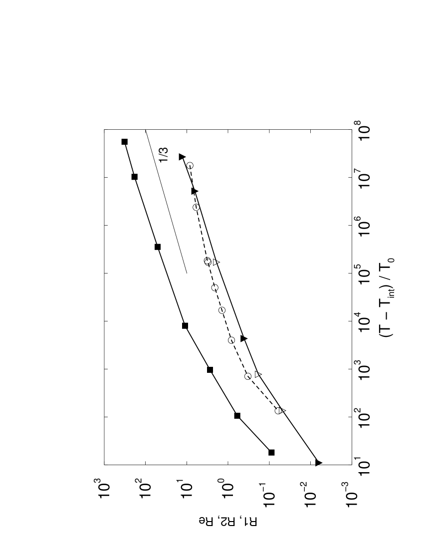
FIG. 3.: Reynolds numbers Re $=l\dot{l}$ (filled squares) for $L=50$ for (left to right) runs in Table I (top to bottom). Ratios $R_{1}$ (circles), $R_{2}$ (triangles), the rms inertial to viscous ratios (see text) at $L=30$ for runs with (left to right) $L_{0}$ = 36, 2.9, 0.59, 0.15, 0.054, 0.024, 0.01, 0.01, 0.0016, 0.00095, 0.00039, 0.0003 (system sizes $96^{3}$ (open) and $128^{3}$ (filled)). Errors are of the order of the symbol size.

The ratio $R_{2}$ is closely related to the Reynolds number Re: it differs in representing length and velocity measures based on the rms fluid flow rather than on the interface dynamics and, because the length scales associated with the velocity gradients are smaller than the domain size, is significantly smaller than Re. The dominance (by a factor ten) of inertial over viscous forces is, at late times, nonetheless clear (Fig.3).

We finally ask whether, at the largest Re values we can reach, there is in fact significant turbulence in the fluid flow. One quantitative signature of turbulence is the skewness $S$ of the longitudinal velocity derivatives; this is close to zero in laminar flow but approaches $S=-0.5$ in fully developed turbulence [18]. We do detect increasingly negative $S$ as Re is increased but reach only $S\simeq-0.3$ for Re $\simeq 350$ [11]. This suggests that at our highest Re’s, turbulence is at most partially developed – a view confirmed by visual inspection of velocity maps [11]. Grant and Elder’s suggestion of an eventual transition to turbulent remixing thus remains open.

In conclusion, we have presented LB simulation data for 3D spinodal decomposition which spans an unprecedented range of reduced time and length scales. At $t\ \raisebox{-0.86108pt}{$\stackrel{{\scriptstyle\scriptstyle<}}{{\scriptstyle\sim}}$}\ 10^{2}$ (Re $\ \raisebox{-0.86108pt}{$\stackrel{{\scriptstyle\scriptstyle<}}{{\scriptstyle\sim}}$}\ 1$) we observe linear scaling, as announced in the previous literature [6, 7, 8, 9]. This is followed by a long crossover ($10^{2}\ \raisebox{-0.86108pt}{$\stackrel{{\scriptstyle\scriptstyle<}}{{\scriptstyle\sim}}$}\ t\ \raisebox{-0.86108pt}{$\stackrel{{\scriptstyle\scriptstyle<}}{{\scriptstyle\sim}}$}\ 10^{6}$, or $1\ \raisebox{-0.86108pt}{$\stackrel{{\scriptstyle\scriptstyle<}}{{\scriptstyle\sim}}$}\$Re$\ \raisebox{-0.86108pt}{$\stackrel{{\scriptstyle\scriptstyle<}}{{\scriptstyle\sim}}$}\ 50$) connecting to a regime in which inertial forces clearly dominate over viscous ones (see Fig.3); our work is the first to unambiguously probe this regime in 3D[10]. In the region so far accessible ($10^{6}\ \raisebox{-0.86108pt}{$\stackrel{{\scriptstyle\scriptstyle<}}{{\scriptstyle\sim}}$}\ t\ \raisebox{-0.86108pt}{$\stackrel{{\scriptstyle\scriptstyle<}}{{\scriptstyle\sim}}$}\ 10^{8}$, or $50\ \raisebox{-0.86108pt}{$\stackrel{{\scriptstyle\scriptstyle<}}{{\scriptstyle\sim}}$}\$Re$\ \raisebox{-0.86108pt}{$\stackrel{{\scriptstyle\scriptstyle<}}{{\scriptstyle\sim}}$}\ 350$) Furukawa’s prediction of $t^{2/3}$ scaling is obeyed, to within simulation error. An open issue is whether this regime marks the final asymptote or whether a further crossover occurs to a turbulent remixing regime (saturating Re) as proposed by Grant and Elder [4]. If it does, we have shown that any limiting value of Re must significantly exceed their estimate of $10-100$.

We thank Craig Johnston, Simon Jury, David McComb, Patrick Warren and Julia Yeomans for valuable discussions. Work funded in part under the EPSRC E7 Grand Challenge.

REFERENCES

- [1] E.D.Siggia, Phys. Rev. A 20, 595 (1979).
- [2] H. Furukawa, Phys. Rev. A 31 1103 (1985); Adv. Phys. 34, 703 (1985).
- [3] A. J. Bray, Adv. Phys. 43, 357 (1994).
- [4] M. Grant and K. R. Elder, Phys. Rev. Lett. 82, 14 (1999).
- [5] See, e.g. K. Kubota, N. Kuwahara, H. Eda and M. Sakazume, Phys. Rev. A 45, R3377 (1992); S. H. Chen, D. Lombardo, F. Mallamace, N. Micali, S. Trusso, and C. Vasi, Prog. Coll. Polymer Sci. 93, 331 (1993); T. Hashimoto, H. Jinnai, H. Hasegawa, and C. C. Han, Physica A 204, 261 (1994).
- [6] M. Laradji, S. Toxvaerd, and O. G. Mouritsen, Phys. Rev. Lett. 77, 2253 (1996).
- [7] S. Bastea and J. L. Lebowitz, Phys. Rev. Lett. 78, 3499 (1997).
- [8] S. I. Jury, P. Bladon, S. Krishna and M. E. Cates, Phys. Rev. E. 59, R2535 (1999).
- [9] The linear law has been reported by a number of groups for which reliable , values are unavailable to us: T. Koga and K. Kawasaki, Phys. Rev. A 44, R817 (1991); S. Puri and B. Dünweg, Phys. Rev. A 45, R6977 (1992); F. J. Alexander, S. Chen, and D. W. Grunau, Phys. Rev. B 48, 634 (1993); linear fits were not offered by C. Appert and S. Zaleski, Phys. Rev. Lett. 64, 1 (1990); A. Shinozaki and Y. Oono, Phys. Rev. Lett. 66, 173 (1991).
- [10] The scaling in 3D has been reported by C. Appert, J. F. Olson, D. H. Rothman, S. Zaleski, J. Stat. Phys. 81 181 (1995); see also, W. Ma, A. Maritan, J. R. Banavar, J. Koplik, Phys. Rev. A 45, R5347 (1992); T. Lookman, Y Wu, F. J. Alexander, S. Chen, Phys. Rev. E 53 5513 (1996); none reliably establish dominance of inertial over viscous forces.
- [11] V. M. Kendon, J-C. Desplat, P. Bladon and M. E. Cates, in preparation.
- [12] P. Bladon and J-C. Desplat, in preparation.
- [13] F. J. Higuera, S. Succi and R. Benzi, Europhys. Lett., 9 345 (1989).
- [14] M. R. Swift, E. Orlandini, W. R. Osborn and J. Yeomans, Phys. Rev. E 54, 5041 (1996).
- [15] A. J. Ladd, J. Fluid Mech., 271, 285 (1994).
- [16] The diffusive contribution for each run was found by running a simulation with the same , but extremely high viscosity; the data were found to fit well to diffusive scaling () and the relevant diffusive growth rate found as ; data from the main runs with was then rejected. (Repeating the analysis with a threshold of 1% did not alter the fit parameters beyond estimated errors.)
- [17] A breakdown of scaling, for different reasons, was also found in two dimensions; A. J. Wagner and J. M. Yeomans, Phys. Rev. Lett. 80, 1429 (1998).
- [18] See e.g. A. S. Monin and A. M. Yaglom, Statistical Fluid Mechanics vol. 2 ed. J. Lumley, MIT Press, Cambridge, MA (1975).
- [19] In discussing the two-dimensional results of H. Furukawa, Phys. Rev. E 55, 1150 (1997), Grant and Elder [4] suggest that, whenever in a simulation in lattice units, the Reynolds number should be “more realistically estimated” by making the replacement . Presumably this is intended to account for non-resolution of the dissipation scale; if so, it is the wrong criterion. One instead requires , which is always true in our work.