Incentive Systems in Multi-Level Markets for Virtual Goods

Abstract.

As an alternative to rigid DRM measures, ways of marketing virtual goods through multi-level or networked marketing have raised some interest. This report is a first approach to multi-level markets for virtual goods from the viewpoint of theoretical economy. A generic, kinematic model for the monetary flow in multi-level markets, which quantitatively describes the incentives that buyers receive through resales revenues, is devised. Building on it, the competition of goods is examined in a dynamical, utility-theoretic model enabling, in particular, a treatment of the free-rider problem. The most important implications for the design of multi-level market mechanisms for virtual goods, or multi-level incentive management systems, are outlined.

1. Introduction

Information goods share the attributes of transferability and non-rivalry with public goods, and additionally are durable, i.e., show no wear out by usage or time [1, 2]. Like with a private good, however, original creation can be costly, whereas reproduction and redistribution are cheap. This is the more true for virtual goods [3], i.e., information goods in intangible, digital form, which are distributed through electronic networks. Free-rider phenomena and “piracy” plague their creators and distributors, a problem which is conventionally approached using copy protection measures and/or digital rights management (DRM) systems which, generally speaking, aim at restoring some of the features of private, physical goods. This practise, backed by WIPO treaties [4] and national copyright law in signatory states giving DRM techniques protected legal status, has aroused public controversy and an ongoing scientific discussion about its various fundamental [5], economic [6], and pragmatic problems [7], cf. [8] for a more general discussion of the underlying concepts of intellectual property rights. The general legitimacy of DRM measures which tend to disrupt consumers’ expectations on their individual usage of the good [9], is doubtful in light of empirical findings on the effect of illegal file-sharing on record sales [10], which seems negligible. Therefore, as an alternative to the protection of virtual goods by DRM, so called incentive management (IM) systems have recently emerged. They promise to yield a fair remuneration to the originator of the good, who may be identical with its creator or not, without necessitating copy protection or disruption of users’ expectations on “fair” and “personal” uses. One of the first such systems, and one which is already in practical use is the so called Potato System [11, 12]. It is based on super distribution of the virtual good from buyer to buyer, whereby each buyer obtains, along with the good itself, the right to redistribute it on commission. Upon resale, she will obtain a share of the purchase price as an additional incentive. The rationale behind this kind of scheme, called here multi-level IM systems, is as obvious as appealing. Rather than to discourage illegal distribution of the good by more or less unpopular measures, the aim is to make legal distribution more attractive than “piracy” [13]. Concurrently, the scheme purports to attribute a fair remuneration to the party from which the good originated, for instance the creator of a work of which the virtual good is an embodiment.

The present report contributes a building block to the presently lacking study of multi-level IM in the framework of theoretical economy. Section 2 introduces a simple model for the monetary flux in a general multi-level market and derives the most basic results pertaining to it. The model is complemented by a dynamical model for the competition of two goods in such a market in Section 3, with particular consideration of virtual goods. Two important special cases are treated in Section 4. Section 4.1 covers the free-rider problem and the potential of multi-level IM to counter it, while Section 4.2 gives a first account of genuine competition between two goods. Section 5 offers a qualitative discussion of the issues raised in the preceding theoretical ones. It is argued in Section 5.1 that, judged on grounds of the theoretical analysis, multi-level IM can be a fair scheme despite its similarity to pyramid schemes. The free-rider problem is recast as an issue of information economy in Section 5.2. Section 5.3 offers some thoughts on the general potential of multi-level IM to influence markets through determining the incentive via dynamical forward pricing. A particular problem of multi-level markets, namely cannibalisation by a potent reseller, is alluded to in Section 5.4. Section 6 concludes by noting some directions for further work. Proofs, and some technical material, are contained in Appendices A, B, respectively. Figures can be found at the end of the paper.

2. Monetary Flux Model

The model we devise is continuous and kinematic in nature. That means firstly, that we describe all pertinent quantities by variables with continuous range. Secondly, that it describes the monetary flux between the market players, and other relevant quantities, such as the expected resales revenue, are to be derived from the kinematics.

About the market players no special assumptions are made, in particular with regard to their decision making processes. That is, the model is neutral with respect to the detailed structure of the monopolist firm marketing the good (which we called its originator), and the consumer buying it. Thus the agents are solely discriminated by the time $t$ at which they enter the market, i.e., buy the good from another agent already present in it. Consequently, buying the good happens only once for each agent, while resale can happen to arbitrary amounts at subsequent times. The market in turn is assumed to be homogeneous, i.e., all agents have equal probability to trade with each other. In accordance, no special market dynamics is assumed by letting the number $n(t)$ of agents in the market at time $t$ be an unspecified function with continuous, non-negative, finite or infinite range. The resales price at time $t$ is denoted by $\pi(t)$.

The expected (average) monetary incentive $v_{i}$ for an agent entering the market at time $t$ is given by

$$v_{i}(t)=v_{r}(t)-\pi(t),$$

that is, the expected revenue $v_{r}$ from resales to agents entering the market at later times, diminished by the price at which the good was bought, i.e., the resales price at time $t$. To calculate $v_{r}$, note that the influx of agents into the market is given by $\dot{n}(t^{\prime})=\mathrm{d}n(t^{\prime})/\mathrm{d}t^{\prime}$ at any later time $t^{\prime}>t$, and if the agent was alone then one could integrate $\pi(t^{\prime})\dot{n}(t^{\prime})$ over an interval to obtain the resale revenue accumulated in it. But since there is competition in the reseller market, and all $n(t^{\prime})$ agents have equal probability to strike a deal with the newcomers, the integrand must be divided by $n(t^{\prime})$. Thus

$$v_{r}(t)=\int_{t}^{\infty}\frac{\pi(t^{\prime})}{n(t^{\prime})}\dot{n}(t^{\prime})\,\mathrm{d}t^{\prime}.$$

Reparametrisation by the monotonously increasing number of agents $n(t)$, makes the independence of the market dynamics manifest and yields

$$v_{r}(n)=\int_{n}^{n_{\infty}}\frac{\pi(n^{\prime})}{n^{\prime}}\,\mathrm{d}n^{\prime},$$

in which the market size $n_{\infty}$ may be finite or infinite.

The model neither specifies all the endogenous and exogenous dynamically changing factors that may contribute to a complete model of multi-level markets, nor does it presume any special estimators for them. Accordingly, the fundamental price function $\pi$, as well as the market dynamics, is left completely unspecified and can be generated by any underlying mechanism without affecting any general results derived from the model.

It is instructive to solve the homogeneous equation $v_{i}=0$, corresponding to an expected balance between resales revenues and buying price. In this case, $\pi$ would necessarily have to satisfy the differential equation ${\mathrm{d}\pi(n)}/{\mathrm{d}n}=-{\pi(n)}/{n}$, the unique solution of which is $\pi(n)=\pi(0)/n$. With this solution however, one obtains $v_{i}=-\pi(0)/n_{\infty}$, showing that this $\pi$ is not a solution of the homogeneous equation for $n_{\infty}<\infty$. The same reasoning applies to any constant, nonzero $v_{i}$ and it follows that such a situation is not realisable in a finite market, due to the singular nature of the integral operator defining $v_{i}$. Thus it makes sense to specialise to finite markets, i.e., to take $n_{\infty}<\infty$. Then, a nonsingular re-parametrisation can be applied, replacing $n$ with the market saturation $s=n/n_{\infty}$, $0\leq s\leq 1$. The integral operator $K\colon\pi\longmapsto v_{i}$, a Volterra operator of the second kind, is defined by

$$(K\pi)(s)\mathbin{\smash[t]{\overset{\scriptscriptstyle\mathrm{def}}{=}}}v_{i}(s)=\int_{s}^{1}\frac{\pi(s^{\prime})}{s^{\prime}}\,\mathrm{d}s^{\prime}-\pi(s).$$

As this operator describes a closed market, one would expect it to satisfy a conservation law. In the present case this law takes the form of a game-theoretical zero-sum condition.

Proposition 2.1 (Zero-Sum Condition).

If $\pi$ is bounded then

$$\int_{0}^{1}v_{i}(s)\,\mathrm{d}s=0.$$

The proofs of all statements are easy calculations and are deferred to Appendix A. The zero-sum condition expresses that wins and losses in incentive compensate each other exactly. It is also the main reason why the attempt to obtain a nontrivial solution to the homogeneous equation was bound to fail (notice that $\pi=\pi(0)/n$ is too singular at $0$ to fall in the scope of Proposition 2.1). One important feature of the model is that the incentive is scale-free, i.e., does not depend on $n_{\infty}$.

For regular enough $\pi$, the inverse of $K$ is easily obtained as a solution of the inhomogeneous equation $K\pi=v_{i}$. The derivatives of $\pi$, $v_{i}$, are denoted by $\dot{\pi}$, $\dot{v}_{i}$, respectively.

Proposition 2.2.

$K$ maps $\mathcal{V}\mathbin{\smash[t]{\overset{\scriptscriptstyle\mathrm{def}}{=}}}C^{1}([0,1])$ bijectively onto

$$\mathcal{W}\mathbin{\smash[t]{\overset{\scriptscriptstyle\mathrm{def}}{=}}}\left\{v_{i}\in C^{1}((0,1])\Bigm{|}{\textstyle\int\nolimits_{0}^{1}}v_{i}=0,\ v_{i}=o({\textstyle\frac{1}{s}}),\text{ and }\dot{v}_{i}=O({\textstyle\frac{1}{s}})\ (s\to 0)\right\}.$$

The inverse of $K\colon\mathcal{V}\longrightarrow\mathcal{W}$ is

$$(\check{K}v_{i})(s)\mathbin{\smash[t]{\overset{\scriptscriptstyle\mathrm{def}}{=}}}-\frac{1}{s}\int_{0}^{s}\sigma\dot{v}_{i}(\sigma)\,\mathrm{d}\sigma.$$ (1)

Although nothing in principle prevents a forward monetary flow from earlier market entrants to later ones by negative prices $\pi<0$, the more conventional case is that of positive resale prices. According to the inversion formula in Proposition 2.2, it is sufficient that $\dot{v}$ is non-positive for $\pi$ to remain non-negative, that is positive (non-negative) prices are always obtained if the incentive is (strictly) monotonic decreasing. The necessary and sufficient condition for positive prices reads as follows.

Proposition 2.3.

Let $\pi\in C^{1}([0,1])$. Then, $\pi$ is positive if and only if

$$\frac{1}{s}\int_{0}^{s}v_{i}(\sigma)\,\mathrm{d}\sigma>v_{i}(s)\quad\text{for all }s.$$

This result has a rather direct interpretation. It says that the monetary flow is always directed backwards if and only if the expected incentive at a certain time is smaller than the average expected incentive before that time.

The basic model can easily amended by further features. In particular it is desirable to take transaction costs and a commission into account. The former can be easily incorporated as follows. In the resale process, the buyer as well as the seller can incur transaction costs. We show how both of these additional costs can be incorporated in the model when they are constant. While the buyer’s transaction cost $\beta\geq 0$ directly adds to the price $\pi(s)$ and can therefore be absorbed in that function, the seller’s transaction cost $\sigma\geq 0$ modifies the integrand for the calculation of $v_{r}$ from $\pi(s)/s$ to $(\pi(s)-\sigma)/s$. Upon integration, this yields a negative contribution in the incentive of the form

$$v_{i}(s)=\int_{s}^{1}\frac{\pi(s^{\prime})}{s^{\prime}}\,\mathrm{d}s^{\prime}+\sigma\ln s-\pi(s).$$

If there is an entity, called the collector, which collects part of the resales revenue, e.g., to remunerate the creator of the good, and pays only part of it as a commission to resellers, the market turns into an open system. The commission factor $0\leq\gamma\leq 1$ diminishes the revenue of a single resale from $\pi$ to $\gamma\pi$, and the modified operator $K_{\gamma}$ yielding the incentive $v_{i,\gamma}$ becomes

$$(K_{\gamma}\pi)(s)=\int_{s}^{1}\frac{\gamma(s^{\prime})\pi(s^{\prime})}{s^{\prime}}\,\mathrm{d}s^{\prime}-\pi(s).$$

Its inverse for differentiable $\pi$ can still be calculated as

$$(\check{K}_{\gamma}v_{i,\gamma})(s)=-\mathrm{e}^{-\int_{0}^{s}\frac{\gamma(\tau)}{\tau}\,\mathrm{d}\tau}\int_{0}^{s}\dot{v}_{i,\gamma}(\sigma)\mathrm{e}^{\int_{0}^{\sigma}\frac{\gamma(\tau)}{\tau}\,\mathrm{d}\tau}\,\mathrm{d}\sigma.$$ (2)

For constant commission this reduces to

$$(\check{K}_{\gamma=\text{const.}}v_{i,\gamma})(s)=-\frac{1}{s^{\gamma}}\int_{0}^{s}\dot{v}_{i,\gamma}(\sigma)\sigma^{\gamma}\,\mathrm{d}\sigma.$$

The amount of money $v_{c,\gamma}$ taken out of the market by the collector can be calculated, e.g., when $\pi$ is bounded, as in Proposition 2.1 to obtain

$$v_{c,\gamma}=\int_{0}^{1}\bigl{(}(K-K_{\gamma})\pi\bigr{)}(s)\,\mathrm{d}s=\int_{0}^{1}\bigl{(}1-\gamma(s^{\prime})\bigr{)}\pi(s^{\prime})\,\mathrm{d}s^{\prime},$$

as expected. Note that this quantity is still normalised and the gross commission collected is $n_{\infty}v_{c,\gamma}$. The market with commission no longer satisfies the zero-sum condition but rather its analogue

$$\int_{0}^{1}v_{i,\gamma}(s)\,\mathrm{d}s=-v_{c,\gamma},$$

balanced with the collector’s share.

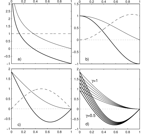
Figure 1. Examples for prices $\pi$ (dashed), expected resales revenues $v_{r}$ (thin solid), and incentives $v_{i}$ (thick solid). a) $\pi=1$, $v_{r}=-\ln s$, $v_{i}=-\ln s-1$. b) $\pi(s)=\sin(\pi s)/(\pi s)-\cos(\pi s)$, $v_{r}=\sin(\pi s)/(\pi s)$, $v_{i}=\cos(\pi s)$. c) $\pi(s)=\sin(\pi s)$, $v_{r}=\operatorname{Si}(\pi)-\operatorname{Si}(\pi s)$, $v_{i}=\operatorname{Si}(\pi)-\operatorname{Si}(\pi s)-\sin(\pi s)$, where $\operatorname{Si}$ is the integral sine function. d) Price as in c) with commission factor $\gamma$ varying from $1$ to $0.5$ in steps of size $0.1$.

A continuous model is an idealisation of a realistic market where buyers enter one by one, i.e., the market size evolves in discrete steps. This entails artifacts, most notably the logarithmic singularity for $v_{i}(s)$ as $s\searrow 0$ when $\pi(0)>0$, see Figure 1 a). Therefore one needs to examine the discrepancy between the incentive obtained from the continuous model and the one calculated by discrete summation somewhat more closely. For a constant price $\pi(s)=\pi$, the discrete model can be solved directly. Agents are labelled with $k=1,\ldots,n_{\infty}$, by the order of market entrance, and this yields for the expected incentive $\overline{v}_{i}$ of the discrete case

$$\overline{v}_{i}=\pi\left(\sum_{k^{\prime}=k+1}^{n_{\infty}}\frac{1}{k^{\prime}-1}-1\right)=\pi\left(\Psi(n_{\infty})-\Psi(k)-1\right),$$

where the Digamma function $\Psi(z)=\Gamma^{\prime}(z)/\Gamma(z)$ is the logarithmic derivative of the Gamma function, see [14, p. 39].

In the general case, we have to look at the difference between $v_{i}(s)$ and the discrete incentive $\overline{v}_{i}(s\cdot n_{\infty})$ at the corresponding point.

Proposition 2.4.

For bounded, non-negative $\pi$ holds

$${\mathord{\left|v_{i}(s)-\overline{v}_{i}(sn_{\infty})\right|}}\leq\frac{\pi_{\mathrm{max}}}{2}\left[\frac{1+s}{sn_{\infty}}+\frac{1}{6}\frac{1+s^{2}}{(sn_{\infty})^{2}}+O\left(\frac{1+s^{4}}{(sn_{\infty})^{4}}\right)\right],$$

with $\pi_{\mathrm{max}}\mathbin{\smash[t]{\overset{\scriptscriptstyle\mathrm{def}}{=}}}\max_{s\in[0,1]}\pi(s)$, and in which the term of order $(sn_{\infty})^{4}$ is strictly dominated by the previous one.

Te error behaviour of the continuous model is rather benign in that it decays with the inverse of the market size at any finite saturation $s>0$. For fixed $k=sn_{\infty}$ on the other hand, a constant error bounded by $c_{k}\pi_{\mathrm{max}}$ for some $c_{k}>0$, will always remain.

The dynamics of multi-level markets are prone to be influenced, if not dominated, by network effects [15], and it is desirable to assess how the incentive relates to them. Network effects are understood in the economics literature as the benefit that accrues to a user of a good or a service because he or she is one of the many who use it. Simple functional forms of network effects for special types of networks, e.g., telecommunication networks, such as Sarnoff’s, Metcalfe’s, and Reed’s law, are often taken as heuristics to explain the dynamics of the growth of networks of the respective type. The most prominent phenomena traced back in this way to network effects are a “slow startup”, the existence of a “critical mass” [16], and strong (supra-exponential) growth after this mass has been reached. Models for network externalities and their effects on prices and utility are numerous and detailed, see, e.g., [17, 18] and references therein, while global models, such as [19] for the possible functional forms of network externalities, are scarce.

Network utility can spatially either be understood in a global sense as the aggregate value, summed over all members of the network, or as the local, individual value enjoyed by its single members. In the present context, each case is in turn subdivided on the temporal axis into the dynamic utility given as a function of the saturation $s$, as a relative variable, and the kinematic utility, which is the scaling behaviour of the utility with the market size $n_{\infty}$.

The aggregate utilities are the simpler ones to discuss. In fact, the only kinematic aggregate utility in our model is that obtained by the replication of the good and distribution of it to the members of the network, a contribution which is always of order $O(n_{\infty})$, like in broadcast networks. The incentive contributes to aggregate utilities only in a dynamic way, since it is given by

$$n_{\infty}\cdot\int_{0}^{s}v_{i}(s^{\prime})\,\mathrm{d}s^{\prime},$$

which approaches zero for $s\to 1$ due to the zero-sum condition, or is of the order $O(-n_{\infty})$, more precisely $-n_{\infty}v_{c,\gamma}$, if a commission is in effect.

The dynamic, individual utility of the network is directly affected by $v_{i}$. In fact, in the continuous model there is no other relevant external contribution to individual utility, since the kinematic, individual utility, defined as the scaling behaviour of $v_{i}$ with $n_{\infty}$, is $O(1)$ precisely if $\pi$ is $O(1)$ $(n_{\infty}\to\infty)$, i.e., if the price stays bounded as the market grows. While this argument holds for large saturations, some care has to be taken for low ones. Firstly, it might be that the continuous model introduces artifacts that lead to nontrivial scaling for small $s=k/n_{\infty}$, keeping $k$ fixed while letting $n_{\infty}$ grow. This is however excluded by the error bound obtained in Proposition 2.4. The scale-free behaviour of the continuous model is therefore stable for nonzero $s$. For small, fixed $k=sn_{\infty}$, and if $\pi(0)>0$ a scaling of the kinematic, individual utility of order $O(\ln n_{\infty})$ is obtained. This is in accordance with the conventional wisdom that in pyramid schemes the profiteers realise profits which scale logarithmically with the number of participants. In conclusion, the incentive introduces a single, independent network externality which, except for a rather moderate effect on early subscribers, does not exert a strong effect on the market. This was to be expected since the market describes has no special structural properties.

Figure 1 a) shows the most basic example of resales revenues and incentives resulting from a constant price. It exhibits the logarithmic singularity present in the continuous model, and which will always emerge if $\pi(0)$ is positive. The singularity is avoided if $\pi(0)=0$ as in b) and c). Additionally, in c) the incentive is forced to zero as $s\to 1$ by letting $\pi$ approach zero, and also shows a case where $v_{i}$ is not always monotonic decreasing and $\pi$ is still positive. The effect of a commission factor is exhibited in Figure 1 d).

3. Competition Model

To devise a dynamical model for the competition of two goods, say $A$ and $B$, in a multi-level market described by the model above, an utility-theoretic approach is suitable. Let $\mathord{{\mathord{s}}^{\bullet}}$ ($\bullet=A$ or $B$) denote the partial market sizes, or market shares for good $A$, and $B$, respectively. As all other variables introduced below, they are considered as dependent variables ${\mathord{{\mathord{s}}^{\bullet}}}={\mathord{{\mathord{s}}^{\bullet}}}(s)$ satisfying ${\mathord{{\mathord{s}}^{A}}}+{\mathord{{\mathord{s}}^{B}}}=s$. This account manifestly treats $A$ and $B$ as substitute goods, i.e., agents decide exclusively for either one or the other.

To describe the decision probability ${\mathord{{\mathord{\rho}}^{\bullet}}}={\mathord{{\mathord{\rho}}^{\bullet}}}(s)$ for buying $A$ or $B$, respectively, at saturation $s$, at least three factors need to be taken into account. The first is the distribution of the genuine, individual utilities ${\mathord{{\mathord{u}}^{\bullet}}}$ of the good across the population. The second is the individual utility ${\mathord{u_{i}^{\bullet}}}\mathbin{\smash[t]{\overset{\scriptscriptstyle\mathrm{def}}{=}}}{\mathord{u_{r}^{\bullet}}}-{\mathord{{\mathord{\pi}}^{\bullet}}}$ originating from individual utilities ${\mathord{u_{r}^{\bullet}}}$ arising from expected resales revenues, where ${\mathord{{\mathord{\pi}}^{\bullet}}}={\mathord{{\mathord{\pi}}^{\bullet}}}(s)$ is the price of the respective goods. In the present model these two factors are considered as exogenous ones, while the third one is an endogenous, generic network effect, captured in a contribution ${\mathord{u_{m}^{\bullet}}}$ to the utility. It is convenient to introduce, for all utilities, the bias $\Delta x\mathbin{\smash[t]{\overset{\scriptscriptstyle\mathrm{def}}{=}}}x^{A}-x^{B}$ as a measure for the advantage gained by deciding for $A$ rather than $B$.

Let ${\mathord{{\mathord{\mu}}^{\bullet}}}={\mathord{{\mathord{\mu}}^{\bullet}}}({\mathord{{\mathord{u}}^{\bullet}}})$ be the probability density function (PDF) of the distribution of $\mathord{{\mathord{u}}^{\bullet}}$ across the population. The distributions for both goods are taken to be equal and to depend only on the respective popularities ${\mathord{{\mathord{p}}^{\bullet}}}\geq 0$, i.e., ${\mathord{{\mathord{\mu}}^{\bullet}}}({\mathord{{\mathord{u}}^{\bullet}}})={\mathord{\mu}}({\mathord{{\mathord{p}}^{\bullet}}},{\mathord{{\mathord{u}}^{\bullet}}})$. We assume that ${\mathord{\mu}}(x)=0$ for $x<0$, and that $\mathord{\mu}$ satisfies the principle of stochastic dominance, i.e.,

$${\mathord{\mathcal{M}}}(q,x)\geq{\mathord{\mathcal{M}}}(p,x)\quad\text{for }p\geq q,$$

where ${\mathord{\mathcal{M}}}({\mathord{p}},x)=\int_{0}^{x}{\mathord{\mu}}({\mathord{p}},y)\mathrm{d}y$ is the cumulative density function (CDF) of $\mathord{\mu}$. With these settings, the probability that an agent decides to buy $A$ is ${\mathord{{\mathord{\rho}}^{A}}}(\Delta)\mathbin{\smash[t]{\overset{\scriptscriptstyle\mathrm{def}}{=}}}\Pr(\Delta u+\Delta>0)$, where the decision bias $\Delta$ subsumes all other utility contributions to the bias for $A$. It follows, with the notation ${\mathord{{\mathord{\rho}}^{A}}}({\mathord{{\mathord{p}}^{A}}},{\mathord{{\mathord{p}}^{B}}};\Delta)={\mathord{{\mathord{\rho}}^{A}}}(\Delta)$, making the dependency of $\mathord{{\mathord{\rho}}^{A}}$ on the popularities explicit,

$${\mathord{{\mathord{\rho}}^{A}}}({\mathord{{\mathord{p}}^{A}}},{\mathord{{\mathord{p}}^{B}}};\Delta) =\int_{0}^{\infty}\mathrm{d}{\mathord{{\mathord{\mu}}^{A}}}(u)\int_{0}^{u+\Delta}{\mathord{{\mathord{\mu}}^{B}}}(u^{\prime})$$ (3)

$$=\int_{0}^{\infty}\mathrm{d}{\mathord{{\mathord{\mu}}^{A}}}(u){\mathord{{\mathord{\mathcal{M}}}^{B}}}(u+\Delta)=\int_{0}^{\infty}\mathrm{d}{\mathord{{\mathord{\mu}}^{A}}}(u){\mathord{\mathcal{M}}}(u+\Delta-{\mathord{{\mathord{p}}^{B}}}).$$

In simple models as used below, the distributions $\mathord{{\mathord{\mu}}^{\bullet}}$ are given in translation form ${\mathord{\mu}}({\mathord{{\mathord{p}}^{\bullet}}},{\mathord{{\mathord{u}}^{\bullet}}})={\mathord{\mu}}(0,{\mathord{{\mathord{u}}^{\bullet}}}-{\mathord{{\mathord{p}}^{\bullet}}})$, in which case (3) simplifies to

$${\mathord{{\mathord{\rho}}^{A}}}({\mathord{{\mathord{p}}^{A}}},{\mathord{{\mathord{p}}^{B}}};\Delta)=\int_{0}^{\infty}\mathrm{d}{\mathord{\mu}}(u){\mathord{\mathcal{M}}}(u+\Delta+\Delta{\mathord{p}}),$$ (4)

where $\Delta{\mathord{p}}={\mathord{{\mathord{p}}^{A}}}-{\mathord{{\mathord{p}}^{B}}}$ is the popularity bias.

Proposition 3.1.

The function ${\mathord{{\mathord{\rho}}^{A}}}(p,q;\Delta)$ is monotonously increasing in $p$ and $\Delta$, monotonously decreasing in $q$, and satisfies

i) ${\mathord{{\mathord{\rho}}^{A}}}(p,q;\Delta)=1-{\mathord{{\mathord{\rho}}^{B}}}(p,q;\Delta)$,

ii) ${\mathord{{\mathord{\rho}}^{A}}}(p,q;\Delta)=1-{\mathord{{\mathord{\rho}}^{A}}}(q,p;-\Delta)$,

iii) ${\mathord{{\mathord{\rho}}^{A}}}(p,q,\Delta)={\mathord{{\mathord{\rho}}^{B}}}(q,p,-\Delta)$.

Having at hand the probability ${\mathord{{\mathord{\rho}}^{A}}}({\mathord{s}})={\mathord{{\mathord{\rho}}^{A}}}({\mathord{{\mathord{p}}^{A}}}(s),{\mathord{{\mathord{p}}^{B}}}(s);\Delta(s))$ to buy $A$ at a given total saturation, we can write down the fundamental relation governing the dynamics of the multi-level market in which $A$ and $B$ compete.

$${\mathord{{\mathord{s}}^{A}}}(s)=\int_{0}^{s}{\mathord{{\mathord{\rho}}^{A}}}(s^{\prime})\mathrm{d}s^{\prime}.$$ (5)

The second element contributing to the decision bias is the agents’ ex ante estimation of resales revenues and the incentive, thus defining $\mathord{u_{r}^{\bullet}}$ and in turn the resales revenue and incentive bias $\Delta u_{r}$ and $\Delta u_{i}=\Delta u_{r}-\Delta{\mathord{\pi}}$, respectively. Due to limited knowledge about the market situation, agents are bound to behave according to a rule of bounded rationality and using partial information. We choose ${\mathord{u_{r}^{\bullet}}}(s)\mathbin{\smash[t]{\overset{\scriptscriptstyle\mathrm{def}}{=}}}{\mathord{u_{r}^{\bullet}}}(s)\cdot{\mathord{{\mathord{\rho}}^{\bullet}}}(s)$, where ${\mathord{u_{r}^{\bullet}}}$ is the bare resales revenue ${\mathord{u_{r}^{\bullet}}}(s)=\int_{s}^{1}{\mathord{{\mathord{\pi}}^{\bullet}}}/s^{\prime}\mathrm{d}s^{\prime}$. Here, ${\mathord{{\mathord{\rho}}^{A}}}(s)={\mathord{{\mathord{\rho}}^{A}}}({\mathord{{\mathord{p}}^{A}}}(s),{\mathord{{\mathord{p}}^{B}}}(s);0)$, and ${\mathord{{\mathord{\rho}}^{B}}}(s)={\mathord{{\mathord{\rho}}^{A}}}({\mathord{{\mathord{p}}^{B}}}(s),{\mathord{{\mathord{p}}^{A}}}(s);0)$ are the probabilities for buying $A$, $B$, respectively, governed merely by popularity. That is, agents expect to gain the resales revenue of an undisturbed multi-level market of relative size ${\mathord{{\mathord{\rho}}^{\bullet}}}(s)$. Sellers transaction costs, which can be assumed to be of similar magnitude for both goods, and small for virtual ones are neglected, as well as commissions by which we focus on the competition between the goods, exclusively. The assumptions on the agents’ accessible information underlying this Ansatz are i) the price schedules ${\mathord{{\mathord{\pi}}^{\bullet}}}(s)$ are public knowledge, ii) $s$ can be estimated with good precision, as well as iii) ${\mathord{{\mathord{\rho}}^{\bullet}}}(s)$. While i) depends on the mechanism implemented by the multi-level IM system, ii) and iii) can be justified to the end that they represent information accessible through local measurements within an agent’s communication reach. Summarising, this definition of $\mathord{u_{r}^{\bullet}}$ represents partially but rather well informed individuals which behave subjectively rational. Further discussion of $\mathord{u_{r}^{\bullet}}$ is contained in Sections 5.1 and 5.2.

As already alluded to in Section 2, the dynamics of multi-level markets is very likely to be affected by network effects. In fact, in a completely homogeneous market and in the absence of other externalities influencing an agent’s decision, a network effect becomes dominant. For, if resellers of good $A$, say, are rare then a buyer will be very likely to buy from a reseller of $B$. In such a situation $\mathord{{\mathord{\rho}}^{A}}$ can become negligible and the market completely governed by the multiplier effect of resellers of $B$. We do not presume such an extreme effect to be prevalent, and, since generic utility-theoretic treatments of network effects are lacking except for special cases, cf. [17, 16, 18], we choose an ad hoc, moderate multiplier utility ${\mathord{u_{m}^{\bullet}}}\mathbin{\smash[t]{\overset{\scriptscriptstyle\mathrm{def}}{=}}}{\mathord{\varepsilon}}{\mathord{{\mathord{s}}^{\bullet}}}/{\mathord{s}}$ depending on an adjustable parameter ${\mathord{\varepsilon}}$. This yields a multiplier bias $\Delta u_{m}={\mathord{\varepsilon}}({\mathord{{\mathord{s}}^{A}}}-{\mathord{{\mathord{s}}^{B}}})/{\mathord{s}}={\mathord{\varepsilon}}(2{\mathord{{\mathord{s}}^{A}}}/{\mathord{s}}-1)$ as the single endogenous contribution to $\mathord{{\mathord{\rho}}^{A}}$.

With the specification

$$\Delta\mathbin{\smash[t]{\overset{\scriptscriptstyle\mathrm{def}}{=}}}\Delta u_{i}+\Delta u_{m}={\mathord{u_{r}^{A}}}{\mathord{{\mathord{\rho}}^{A}}}-{\mathord{u_{r}^{B}}}{\mathord{{\mathord{\rho}}^{B}}}-({\mathord{{\mathord{\pi}}^{A}}}-{\mathord{{\mathord{\pi}}^{B}}})+{\mathord{\varepsilon}}\left(\frac{2{\mathord{{\mathord{s}}^{A}}}}{{\mathord{s}}}-1\right)$$ (6)

the model for the competition of two goods in a multi-level IM market is complete. Note that (3), (5), (6) present an exactly solvable integral equation for $\mathord{{\mathord{s}}^{A}}$. Will will now examine some special numerical solutions of it.

4. Two Special Cases

Though the presented competition model is simple, the space of situations covered by it is vast, as input data are the price schedules $\mathord{{\mathord{\pi}}^{\bullet}}$, popularity functions $\mathord{{\mathord{p}}^{\bullet}}$, and the multiplier factor coupling ${\mathord{\varepsilon}}$, but also the dependency of $\mathord{\mu}$ on the popularities. Here we assume that the latter be of translation form (4), and specify that ${\mathord{\mu}}(0,u)$ is given by the special Weibull distribution $f(u;1,2)$, see Appendix B, in which case $\mathord{{\mathord{\rho}}^{A}}$ takes the analytical form (7). For $\mathord{{\mathord{\pi}}^{\bullet}}$ and $\mathord{{\mathord{p}}^{\bullet}}$ we specialise to spike functions

$$g(s;m)\mathbin{\smash[t]{\overset{\scriptscriptstyle\mathrm{def}}{=}}}\begin{cases}s/m,&\text{for $0\leq s\leq m$;}\\ (1-s)/(1-m)&\text{for $m<s\leq 1$.}\end{cases}$$

Pragmatically, $\mathord{{\mathord{\pi}}^{\bullet}}$ of spike form offer an early-subscriber discount and a late-adopter rebate, cf. Section 5.3. Technically, they are the simplest price schedules which avoid an initial singularity, thereby minimising the variance with a discrete model, and correspond to markets closing at finite size.

Besides the market shares ${\mathord{{\mathord{s}}^{\bullet}}}$ and the final shares ${\mathord{S^{\bullet}}}\mathbin{\smash[t]{\overset{\scriptscriptstyle\mathrm{def}}{=}}}{\mathord{{\mathord{s}}^{\bullet}}}(1)$, the turnovers

$${\mathord{t^{\bullet}}}(s)\mathbin{\smash[t]{\overset{\scriptscriptstyle\mathrm{def}}{=}}}\int_{0}^{s}{\mathord{{\mathord{\pi}}^{\bullet}}}(s^{\prime}){\mathord{{\mathord{\rho}}^{\bullet}}}(s^{\prime})\mathrm{d}s^{\prime}=\int_{0}^{s}{\mathord{{\mathord{\pi}}^{\bullet}}}(s^{\prime}){\mathord{\dot{s}^{\bullet}}}(s^{\prime})\mathrm{d}s^{\prime}=\int_{0}^{{\mathord{{\mathord{s}}^{\bullet}}}(s)}{\mathord{{\mathord{\pi}}^{\bullet}}}({\mathord{{\mathord{s}}^{\bullet}}}^{\prime})\mathrm{d}{\mathord{{\mathord{s}}^{\bullet}}}^{\prime}$$

and the total turnovers ${\mathord{T^{\bullet}}}\mathbin{\smash[t]{\overset{\scriptscriptstyle\mathrm{def}}{=}}}{\mathord{t^{\bullet}}}(1)$ are important indicators for the economic performance of the competing goods. Note that the maximal turnover that a good can generate is $1/2$ for spike functions. Furthermore, we examine the discrepancy between agents’ expectation and the actual resales revenue they can achieve, similarly calculated as

$${\mathord{v_{r}^{\bullet}}}(s)\mathbin{\smash[t]{\overset{\scriptscriptstyle\mathrm{def}}{=}}}\int_{s}^{1}\frac{{\mathord{{\mathord{\pi}}^{\bullet}}}(s^{\prime})}{{\mathord{{\mathord{s}}^{\bullet}}}}{\mathord{{\mathord{\rho}}^{\bullet}}}(s^{\prime})\mathrm{d}s^{\prime}=\int_{{\mathord{{\mathord{s}}^{\bullet}}}(s)}^{{\mathord{S^{\bullet}}}}\frac{{\mathord{{\mathord{\pi}}^{\bullet}}}({\mathord{{\mathord{s}}^{\bullet}}}^{\prime})}{{\mathord{{\mathord{s}}^{\bullet}}}^{\prime}}\mathrm{d}{\mathord{{\mathord{s}}^{\bullet}}}^{\prime},$$

and the resulting actual incentive ${\mathord{v_{i}^{\bullet}}}(s)\mathbin{\smash[t]{\overset{\scriptscriptstyle\mathrm{def}}{=}}}{\mathord{v_{r}^{\bullet}}}(s)-{\mathord{{\mathord{\pi}}^{\bullet}}}(s)$.

4.1. Free-Rider Phenomena

To counter free-rider phenomena is the main aim behind the conception of multi-level marketing of virtual goods. In fact, the content distribution network of multi-level IM systems like the Potato system [11, 12, 20] is very similar to the peer-to-peer networks commonly used by free riders [21]. By this rationale, we can compare the performance of a virtual good $A$ with a pirated version $B$ of it in the same multi-level market. That is, the popularities are equal ${\mathord{{\mathord{p}}^{A}}}={\mathord{{\mathord{p}}^{B}}}$ and $B$ is free, i.e., ${\mathord{{\mathord{\pi}}^{B}}}=0$. Since in this case no confusion can arise, we sometimes drop the superscript $A$.

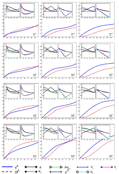
Figure 3. Example market evolutions in the free-rider setting.

Figure 3 shows how the market evolves in this setting for some selected cases. The main figures show the market indicators $s$ and $2t$ (relative to the maximal turnover $1/2$). The left and right inlays exhibit the factors contributing to the decision biases, and the resulting ${\mathord{\rho}}$, respectively, a comparison between expected and actual resales revenues and incentives. The left column has an early peaking price schedule $m=0.1$, entailing an initially very high and then steeply dropping incentive bias (right inlays), while in the centre and right columns $m=0.5$, $0.9$, respectively, which in turns leads to a smaller, but longer lasting positive initial $\Delta u_{i}$. Note the sharp negative peak of $\Delta u_{i}$ for $m=0.9$, entailing a significant entry deterrence, i.e., ${\mathord{\rho}}<0.5$ at late times. The right inlays show that the simple rule for $u_{r}$ leads to good estimations for $v_{r}$, and in turn $v_{i}$. Agents tend to underestimate the resales revenues they can achieve at early times and overestimate them only in an intermediate phase. The increasing influence of multiplier effects can be observed along the four rows for which ${\mathord{\varepsilon}}=0$, $0.3$, $0.6$, $0.9$ from top to bottom.

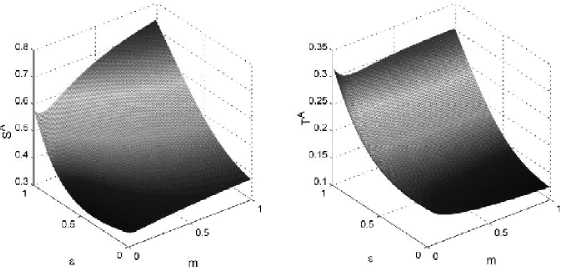
Figure 4. Final shares (left) and total turnovers (right) in the free-rider setting.

Even without a multiplier effect present, the incentive can lead to a non-negligible market share though not dominance. However significant turnovers are not generated without exploiting the multiplier effect by an initial invitation to enter, i.e., a positive incentive at early times. For multiplier biases ${\mathord{\varepsilon}}\cong 1$ which are comparable to the price and other biases, good $A$ can reach market dominance and generate over $1/2$ of the maximum turnover. To maximise turnovers, the price schedule must be aligned with the market growth $\mathord{{\mathord{s}}^{A}}$, which is generally difficult. Figure 4 shows the plateaus of ${\mathord{S^{A}}}$ and ${\mathord{T^{A}}}$ in dependence of $m$ and ${\mathord{\varepsilon}}$. It can be seen that maximisation of turnover and share are conflicting goals.

4.2. Smash Hits and Sleepers

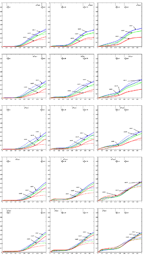
Figure 5. Competition between sleeper and smash hit. Market shares ${\mathord{{\mathord{s}}^{A}}}$ are solid, turnovers $2{\mathord{t^{A}}}$ dashed.

Scenarios for the competition of two goods are manifold within our model and lack of space prohibits a comprehensive treatment. Here, as a familiar example, good $A$ is assumed to have a popularity function peaking later than that of $B$, i.e., $A$ would commonly be termed a ‘sleeper’ while $B$ can be considered a ‘smash hit’. Denote by ${\mathord{m_{p}^{A}}}$, ${\mathord{m_{p}^{B}}}$ the popularity peaks of $A$ and $B$, respectively. The originator of $A$ would like to counter the slow startup effect due to later popularity utilising an appropriate price schedule, corresponding to various positionings of the peak ${\mathord{m^{A}}}$ of his price function. The price function of $B$ is assumed to be centred, ${\mathord{m^{B}}}=0.5$. Examples are shown in Figure 5. It can be seen that the final share of $A$ is mostly small if the multiplier effect is strong, since then the early rise in popularity of $B$ gives $B$ a persistent advantage. To counter this by a long lasting rebate, i.e., a late price peak ${\mathord{m^{A}}}$ is in fact possible, as the first two rows (${\mathord{m^{A}}}=0.9$, ${\mathord{m^{A}}}=0.7$, respectively) show. The opposite strategy to start the market by an early peaking price and therefore high initial incentive can also work, as can be observed in the last two rows (${\mathord{m^{A}}}=0.3$, ${\mathord{m^{A}}}=0.1$, respectively). However in this case, the price function of $A$ is misaligned with the market evolution and hampers the generation of turnovers. In conclusion, to optimise the price function of the sleeper so as to obtain good market shares and turnovers, is difficult.

5. Discussion and Practical Implications

5.1. Pyramid Schemes and the Issue of Fairness

Attractive as it may be, multi-level IM has, some similarity with pyramid sales schemes — a publicly discouraged enterprise, which is illegal under most jurisdictions. Thus the natural question emerges, whether IM systems based on super distribution on commission are a tenable market mechanism at all, and in particular for virtual goods. In practise, the question is whether multi-level IM falls in the economical category of legitimate multi-level marketing (also referred to as direct, or network sales), or of illegal pyramid schemes [22].

The key argument for the defence of multi-level IM is that a buyer acquires not only a void right to resale, but with it a good of positive value, meaning that potential losses he will incur when he enters the market too late, i.e., too close to saturation to obtain significant resales revenues, can be partially alleviated by the good’s value.

An important difference between pyramid schemes operating with physical goods and multi-level IM is clarified through the analysis of transaction costs. The negative contribution of sellers’ transaction costs $-\sigma\ln s$ can hit early buyers very hard, since they have to process many resales. A particular case in the real world to which this finding corresponds is the detrimental effect of inventory loading in pyramid schemes. There [23], resellers of the good incur extraordinarily high transaction costs by being required too keep a large, non-returnable stock of the goods, probably more than they could ever expect to sell. The penalty arising from this multiplies for early adopters who actually sell a portion of the goods and are required to reorder stock, which is then usually possible only in overly large lots. Virtual goods are much tamer in this respect, since the marginal cost for their replication, as well as the transaction cost for resales, are small, if not negligible. Stock keeping in itself is not an issue, since virtual goods allow for principally infinite, lossless replication. Marginal costs for their replication and redistribution are, more often than not, orders of magnitude smaller than their value, even if they are embodied on a physical media like a CD, say, for transport. This is the key difference which makes multi-level IM of virtual goods more viable and acceptable in many cases than analogous multi-level marketing schemes for physical goods. In the Potato system for instance, the processing of resales, including accounting, billing, and charging is fully borne by the central server, for which a percentage of the price is assigned to the system [20]. That is, the transaction costs are absorbed in the commission factor and after a buyer has received his resale link from the system in a one-off transaction, the marginal costs for resales are close to zero.

Thus, the individual utility of the good for the buyers is central to the question of fairness of multi-level IM. If the good’s utility is close to zero, then the scheme cannot be considered fair anymore but resembles a pure Ponzi scheme or “Peter-and-Paul” scam. Formalising, to be fair a multi-level IM scheme should meet the requirement $u_{i}\geq-u$ (on average over the buyer population) if fairness is judged on a subjective level, or $v_{i}\geq-u$ judged from a forensic perspective. This condition limits the scope in which the incentive can be predetermined using dynamical forward pricing in multi-level IM, see Section 5.3 below.

5.2. The Free-Rider Problem

A secondary meaning conventionally attributed to the term incentive, is that the incentive can be used by the principal who places it as a means to eventually meet some ends, in particular to minimise the readiness of agents to take moral hazards, for instance becoming an illegal free-rider [24].

Whether multi-level IM can be successful in meeting the aim to fully replace copy protection measures and conventional DRM is a question for theoretical economy, cf. [25] for a treatment of this question in conventional market settings. If the good is freely available, as, for instance, in the Potato system, then it is not a priori clear that another equilibrium apart from ${\mathord{S^{A}}}=0$ (only free riders) exists. The zero-sum condition tells us that, globally, an agent partaking in the IM market is not worse off on average than one not doing so, and thus a market of any size $n_{\infty}>0$ is in fact a global equilibrium. Assume the agents to be rational and conservative in the sense that they would tend to copy the good for free in the absence of an additional payoff. Then, a necessary condition for the market to evolve is that there is an initial phase of in which they can expect a positive pecuniary incentive, that is $u_{i}(s)>0$ for $s<s_{0}$, $s_{0}>0$.

It is here that the free-rider phenomenon is closely connected to the issue of fairness and the economical purport of information. For if the zero-sum condition is common knowledge, then rational agents would always choose the free good since they know that later potential buyers with negative incentive (actual or subjective) will do so. This renders the success of real pyramid schemes paradoxical, and shows that the incentive schedule is at most public knowledge: There must be agents who know that some others will have a negative incentive but expect them to enter the market nonetheless. This is the reason for modelling the decision mechanism of agents using a rule of bounded rationality, as in Section 3. As shown in Section 4.1, an initial invitation to enter through a positive incentive can, within the scope of this model and if combined with a (small) multiplier effect, turn multi-level IM into a functioning tool to counter the free-rider phenomenon.

The presence of the free version can be seen as an exogenous factor negatively affecting the individual utility $u$, and in turn the scope for the determination of the incentive. This is the classical dilemma for the marketing of digital goods and the one addressed by copy protection and DRM. To offer a pragmatical conjecture, it might make sense to differentiate the freely available version of the good from the one distributed through the multi-level IM system, by adding some value and copy protection to the latter, though this would be a partial return to conventional DRM measures, maybe in the “softer” forms of watermarking, personalisation, and fingerprinting, to enable traceability of illegal copies [5].

5.3. Dynamical Forward Pricing

For the operator of a multi-level IM system, the primary goal to maximise the revenues for the originator of the good through his share of the commissions, contains the secondary sub-goal of promoting the distribution of the good, i.e., maximising the market penetration. A central, new result of the present study is the possibility, via the inversion formulae (1) and (2), to dynamically adapt the incentive during the evolution of the market if the operator of the system controls the price as an external parameter. This is useful to turn multi-level IM systems with dynamical forward pricing into tools for market mechanism design, to achieve the mentioned goals. While dynamical forward pricing is not a new concept in the theory of information goods [26], this possibility has, in the context multi-level incentive markets for virtual or physical goods, not yet been widely considered in the literature.

Figure 1 shows the most basic possibilities for price functions. A constant price as in a) is associated with a strong favouritism of early buyers, while later market entrants are increasingly penalised. A typical example for what is conventionally termed an early subscriber discount is shown in b). In real markets this is often used as a means to spur the distribution of the good in an early stage of market development, i.e., to counteract a slow startup effect. For the marketing of virtual goods, such an initial invitation to enter becomes important, in particular if the good is freely available through legal or illegal channels, and therefore early buyers cannot be sure about their potential resales revenues which depend logarithmically on the market size (remember that $v_{i}(k=sn_{\infty})$ scales as $\ln n_{\infty}$). The price associated with the incentive in b) is monotonous increasing, resulting in a double penalty to later buyers who pay more and receive less incentive. Buyers who enter this market for some reason at late times will notice that they are disfavoured, and possibly tend to become frustrated. The third example in Figure 1 c) improves on b) by letting the price vanish when the market reaches saturation. This $v_{i}$ combines a discount for early subscribers with a rebate for very late ones who finally obtain the good gratuitously. This pricing can therefore potentially be used to spur the distribution of the good in early market phases through low price and high incentive, as well as at late times, when the good itself might have lost in utility and the market looses dynamics. If we assume that the market has a positive growth dynamics in an intermediate phase associated with a high demand and maybe a higher individual utility, then it is also reasonable to let the prices peak and lower the incentive during this phase, as in c). Deepness and position of the minimum of $v_{i}$ can be adjusted almost arbitrarily. Finally, d) shows the relatively limited effect that a collector has on the incentive. In particular it can be seen that the point at which the incentive becomes negative is not significantly shifted by the increasing commission factor.

For an implementation of dynamical forward pricing, information on the market dynamics becomes essential, in particular the current size $n(t)$ of the market must be known. This is in fact the case, e.g., in the Potato system, where a central server counts every single acquisition of the good. A much more difficult to determine variable is the absolute market size $n_{\infty}$, necessary to calculate the saturation $s=n/n_{\infty}$. Although one might try to estimate $n_{\infty}$ by market research, comparison with earlier runs of the system for different goods, or other means of educated guessing, a more pragmatic solution suggests itself. Namely, as in the last example in Figure 1, setting the price to zero after some finite time, respectively at an a priori given $n_{\infty}$ obtains a natural condition for closure of the market.

Market closure in this manner runs somewhat counter to the aim of maximising shares yet the effect on the turnover can be limited if the price becomes small enough at late times. Market closure yields the additional benefit of effectively rewarding late buyers by a rebate, which makes additional sense when looking beyond the level of a single run if the IM system. Then, the possible frustration of late buyers with low $v_{i}$ might deter them from partaking in the IM market for a following good. Note that such a procedure is not too uncommon for goods whose value is to a large extent determined by its information content — although on a larger timescale than we would envisage for multi-level IM. For instance, many academic publishers are now distributing classic scholarly titles for free. Also, many legal codifications of intellectual property rights foresee a forfeiture after a certain period.

Information is an essential tool for running a multi-level IM system. It is desirable to decouple the agents’ decisions from the price and bind it more strongly to the incentive. For that, a precondition is the proper information of the market about the expected incentive, that is, viable IM depends to some extent on market transparency. The examples of Section 4 show that agents can have a rather precise estimate on their incentive using local information. The operator of a multi-level IM system could support this by providing some information of his own, but perhaps not all, since particularly the absolute market size of a certain is a potentially useful information for competitors. Namely, in a competitive situation the additional difficulty arises that the $s$ cannot be determined by a single party which may at best know its own partial market size. For instance, in order to avoid closing the market to early, close observation of competitors prices, respectively, activity of peer-to-peer networks distributing the good to free riders, becomes indispensable.

Mixed forms of dynamical price settings can be envisaged, e.g., a positive correlation of $\pi$ with the buying frequency, combined with a frequency or price threshold below which the price is set to zero and the market closed. In any case, as Section 4.1 and Section 4.2 showed designing the optimal price schedule is a complex task, in particular in competitive situations.

5.4. Roots and Market Cannibalisation

For the originator of the good, whom we assume for the time being also to control the IM system, there are basically two ways to extract revenues from the market: He can either act as the market’s root. That is he is the first reseller, paying himself a price equal to the original production cost of the good. Or he can use a commission model (combinations of both cases are of course thinkable). The analysis of network effects yields an argument that the former possibility is in principle inferior to the latter. For the originator’s revenues scale with the total revenues in the market as $O(n_{\infty})$ for large market sizes, while the revenues of a root go only with $O(\ln n_{\infty})$. This is in essence a consequence of the fact that a pure multi-level market cannot easily be monopolised by a single reseller, or even a group of them. In turn it explains why commission models are a standard practise in multi-level marketing.

This leads us to a caveat with respect to the crucial assumption underlying our market model, namely homogeneity. If the market is biased in the sense that there are groups of agents with systematically higher trading capacities than others, this assumption breaks down. Heuristically, considering only an average agent in a structureless market should be a good approximation if the number of potential participants is large and consists of a more or less homogeneous group of individuals, like one with special personal preferences, e.g., musical. In practise, large music labels running direct sale web sites are the counterexample where this heuristics is most blatantly violated. If such a label concurrently offers one of their titles through a multi-level IM system, the chances of the average buyer to buy from this root source are much higher than to meet any other market participant. The same argument exhibits the imminent danger that the market can be cannibalised at an early stage by a player with overwhelmingly high communication capacity, e.g., a popular web site, who could then obtain a practical monopoly. Some studies indicate that monopoly creation could be a rather natural effect in e-commerce [27]. While the originator of the good is not too affected by this phenomenon if he uses a commission model, the other buyers’ incentives are always negatively affected. To what extent the market can be levelled by means of the IM system, e.g., by providing equal communication capacities to all participants, restricting or controlling resale volumes or frequencies, etc., warrants separate discussion.

6. Conclusions

Let us briefly note some directions for further work. On the theoretical side it would be desirable to improve the both the monetary flux model and the competition model to account for, e.g., market inhomogeneities in the former and further externalities’ influence on the decision mechanism of the agents in the latter. In particular, a better justified model for the multiplier effect and a proper incorporation of other network effects is wanting. More refined simulations of multi-level markets in the framework of agent-based computational economics [28], can be useful. A proper treatment of multi-level markets and the competition of goods therein from the viewpoint of theoretical economics should also answer questions of optimality, equilibria, and their stability. The free-rider problem in multi-level IM should also be treated in a more theoretical approach using the principal-agent model [24] and aiming at describing the effect of the incentive on the moral hazard incurred by the agents.

Pragmatically and in order to design proper market mechanisms and actual systems for multi-level IM, the most daunting task from the present viewpoint is to ensure equal opportunities for resellers in the market, i.e., to practically corroborate the theoretical assumption of homogeneity.

Appendix A Proofs of Propositions

Proof of Proposition 2.1.

For ${\mathord{\varepsilon}}>0$ consider

$$\int_{\mathord{\varepsilon}}^{1}\mathrm{d}s\int_{s}^{1}\frac{\pi(s^{\prime})}{s^{\prime}}\,\mathrm{d}s^{\prime} =\int_{\mathord{\varepsilon}}^{1}\mathrm{d}s^{\prime}\int_{\mathord{\varepsilon}}^{s^{\prime}}\frac{\pi(s^{\prime})}{s^{\prime}}\,\mathrm{d}s$$

$$=\int_{\mathord{\varepsilon}}^{1}\frac{s^{\prime}-{\mathord{\varepsilon}}}{s^{\prime}}\pi(s^{\prime})\,\mathrm{d}s^{\prime}$$

$$=\int_{\mathord{\varepsilon}}^{1}\pi(s^{\prime})\,\mathrm{d}s^{\prime}-{\mathord{\varepsilon}}\int_{\mathord{\varepsilon}}^{1}\frac{\pi(s^{\prime})}{s^{\prime}}\,\mathrm{d}s^{\prime}.$$

If $\pi(s)$ is bounded on $[0,1]$ as assumed then the second term is of order $O({\mathord{\varepsilon}}\ln{\mathord{\varepsilon}})$ and therefore vanishes as ${\mathord{\varepsilon}}\searrow 0$. The first term converges to

$$\int_{0}^{1}\pi(s)\,\mathrm{d}s,$$

as desired. ∎

Proof of Proposition 2.2.

For $\pi\in\mathcal{V}$, $(K\pi)(s)$ is a continuously differentiable function in the interval $(0,1]$ with derivative $-\pi(s)/s-\dot{\pi}(s)$. The latter is of order $1/s$ as $s\searrow 0$ since $\pi$ stays bounded at zero. For the same reason, the integral in $K\pi$ is $O(\ln s)$ $(s\to 0)$, which is $o(1/s)$, showing $(K\pi)(s)=o(1/s)$ $(s\to 0)$. $K\pi$ satisfies the zero-sum condition due to Proposition 2.1. Thus $K\pi\in\mathcal{W}$ and we can apply $\check{K}$ to obtain

$$(\check{K}K\pi)(s) =\check{K}\left(\int_{\sigma}^{1}\frac{\pi(s^{\prime})}{s^{\prime}}\,\mathrm{d}s^{\prime}-\pi(\sigma)\right)$$

$$=-\frac{1}{s}\int_{0}^{s}\left(-\frac{\pi(\sigma)}{\sigma}-\dot{\pi}(\sigma)\right)\sigma\,\mathrm{d}\sigma$$

$$=\frac{1}{s}\left(\int_{0}^{s}\pi(\sigma)\,\mathrm{d}\sigma-\int_{0}^{s}\pi(\sigma)\,\mathrm{d}\sigma+\bigl{[}\pi(\sigma)\sigma\bigr{]}_{0}^{s}\right)$$

$$=\pi(s).$$

On the other hand, if $\dot{v}_{i}=O(1/\sigma)$ $(\sigma\to 0)$, then the last calculation showed that $\check{K}$ can be applied to it and obtains a differentiable function in $(0,1)$ which extends continuously to $[0,1]$. That is $\check{K}v_{i}\in\mathcal{V}$ and we calculate for $s>0$

$$(K\check{K}v_{i})(s) =-\int_{s}^{1}\frac{1}{s^{\prime 2}}\int_{0}^{s^{\prime}}\sigma\dot{v}_{i}(\sigma)\,\mathrm{d}\sigma\,\mathrm{d}s^{\prime}+\frac{1}{s}\int_{0}^{s}\sigma\dot{v}_{i}(\sigma)\,\mathrm{d}\sigma$$

$$=-\int_{s}^{1}\dot{v}_{i}(s^{\prime})\,\mathrm{d}s^{\prime}+\int_{0}^{1}\sigma\dot{v}_{i}(\sigma)\,\mathrm{d}\sigma$$

$$=v_{i}(s)-v_{i}(1)+\lim_{{\mathord{\varepsilon}}\searrow 0}\left(-\int_{\mathord{\varepsilon}}^{1}v_{i}(\sigma)\,\mathrm{d}\sigma+\bigl{[}\sigma v_{i}(\sigma)\bigr{]}_{\mathord{\varepsilon}}^{1}+\int_{0}^{\mathord{\varepsilon}}\sigma\dot{v}_{i}(\sigma)\,\mathrm{d}\sigma\right)$$

In the last step, we used continuity of $$v_{i} 1 v_{i}=o(1/\sigma) \dot{v}_{i}=O(1/\sigma) (\sigma\to 0)$$ at . Now, since , , the limit can be assumed and yields

$$=v_{i}(s)-v_{i}(1)+\int_{0}^{1}v_{i}(\sigma)\,\mathrm{d}\sigma+v_{i}(1)$$

$$=v_{i}(s),$$

where the zero-sum condition has been used. ∎

Proof of Proposition 2.3.

Partial integration yields

$$\int_{0}^{s}\sigma\dot{v}_{i}(\sigma)\,\mathrm{d}\sigma=\int_{0}^{s}v_{i}(\sigma)-sv_{i}(s),$$

where we have used that $\sigma v_{i}(\sigma)\to 0$ for $\sigma\searrow 0$ if $\pi$ is $C^{1}$, cf. Proposition 2.2. The result follows upon inserting the above equation into the inequality $\pi(s)>0$ and using Proposition 2.2. ∎

Proof of Proposition 2.4.

We have for $sn_{\infty}$ integer

$${\mathord{\left|v_{i}(s)-\overline{v}_{i}(sn_{\infty})\right|}} ={\mathord{\left|\int_{s}^{1}\frac{\pi(s^{\prime})}{s^{\prime}}\,\mathrm{d}s^{\prime}-\sum_{k^{\prime}=sn_{\infty}+1}^{n_{\infty}}\frac{\pi(k^{\prime}/n_{\infty})}{k^{\prime}-1}\right|}}$$

$$=\lim_{{\mathord{\varepsilon}}\searrow 0}{\mathord{\left|\int_{s}^{1+{\mathord{\varepsilon}}}\pi(s^{\prime})\left(\frac{1}{s^{\prime}}-\sum_{k^{\prime}=sn_{\infty}+1}^{n_{\infty}}\frac{\delta(s^{\prime}-k^{\prime}/n_{\infty})}{s^{\prime}}\right)\,\mathrm{d}s^{\prime}\right|}}$$

where we extended $$\pi [1,1+{\mathord{\varepsilon}}] \delta \pi$$ continuously in a small interval , and used Dirac’s -function to incorporate the sum in the integral. Now, the non-negative factor can be drawn out to estimate

$$\leq\pi_{\mathrm{max}}{\mathord{\left|\Psi(sn_{\infty})-\ln s-\Psi(n_{\infty})\right|}}$$

$$=\pi_{\mathrm{max}}\bigl{(}{\mathord{\left|\Psi(sn_{\infty})-\ln sn_{\infty}\right|}}+{\mathord{\left|\ln n_{\infty}-\Psi(n_{\infty})\right|}}\bigr{)}$$

Using the asymptotic expansion of the $\Psi$ function for $r$ a positive integer, see [14, p. 295], we obtain

$${\mathord{\left|\ln r-\Psi(r)\right|}}\leq\frac{1}{2r}+\sum_{m=1}^{n}\frac{{\mathord{\left|B_{2m}\right|}}}{2mr^{2m}},\quad\text{for }n\geq 0,$$

where $B_{2m}$ is the $2m$-th Bernoulli number. From this follows the claim. ∎

Proof of Proposition 3.1.

The assertions on monotonicity follow from positivity of probability distributions (for $\Delta$) and stochastic dominance (for $p$, respectively, $q$). Symmetries i) and ii), from which iii) follows directly, are easy calculations. ∎

Appendix B Weibull Distribution of Individual Utilities

The Weibull distribution is widely used in reliability and lifetime estimation. It is defined by the PDF

$$f(x;a,b)\mathbin{\smash[t]{\overset{\scriptscriptstyle\mathrm{def}}{=}}}ba^{-b}x^{b-1}\mathrm{e}^{-(x/a)^{b}}\chi_{(0,\infty)}(x),$$

where $\chi_{(0,\infty)}(x)$ is the characteristic function of the positive half axis. For $a=1$, $b=2$ it reduces to the utility distribution used in Section 4

$${\mathord{\mu}}(x)\mathbin{\smash[t]{\overset{\scriptscriptstyle\mathrm{def}}{=}}}f(x;a,b)=2x\mathrm{e}^{-x^{2}}\chi_{(0,\infty)}(x),$$

the CDF of which is

$${\mathord{\mu}}(x)=1-\mathrm{e}^{-x^{2}}\chi_{(0,\infty)}(x).$$

If $\mathord{\mu}$ ($\mathord{{\mathord{p}}^{\bullet}}$,$\mathord{{\mathord{u}}^{\bullet}}$) is given in translation form, formula (4) yields for ${\mathord{{\mathord{\rho}}^{A}}}(\Delta)$, $\Delta\geq 0$,

$${\mathord{{\mathord{\rho}}^{A}}}(\Delta)=1+\frac{\sqrt{2\pi}}{4}\Delta\mathrm{e}^{-\Delta^{2}/2}\left(1-\operatorname{erf}(\Delta/\sqrt{2})\right)-\mathrm{e}^{-\Delta^{2}/2}.$$ (7)

These functions are shown in Figure 2 where it is apparent that $\mathord{{\mathord{\rho}}^{A}}$ is concave for $\Delta>0$, in this case, and ${\mathord{{\mathord{\rho}}^{A}}}(-\Delta)=1-{\mathord{{\mathord{\rho}}^{A}}}(\Delta)$, as follows from Proposition 3.1.

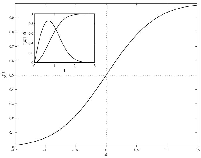
Figure 2. Decision probability ${\mathord{{\mathord{\rho}}^{A}}}(\Delta)$ resulting from popularity distributions given by translates of the Weibull distribution $f(x;1,2)$. The PDF and CDF of $f(x;1,2)$ are shown in the inlay.

References

- [1] C. Shapiro, H. Varian: Information Rules: A Strategic Guide to the Network Economy. Harvard Business School Press, 1999.
- [2] Mark Stegman: Information Goods and Advertising: An Economic Model of the Internet. National Bureau of Economic Research Universities Research Conference “Economics of the Information Economy”, 7 and 8 May 2004, Royal Sonesta Hotel, Cambridge, MA. \hrefhttp://www.nber.org/ confer/2004/URCs04/stegeman.pdfhttp://www.nber.org/ confer/2004/URCs04/stegeman.pdf
- [3] Patrick Aichroth, Jens Hasselbach: Incentive Management for Virtual Goods: About Copyright and Creative Production in the Digital Domain. International Workshop for Technology, Economy, Social and Legal Aspects of Virtual Goods, 27–29 May 2003, Technical University Ilmenau, Germany, on-line publication, pp. 70–81. \hrefhttp://virtualgoods.tu-ilmenau.de/2003/incentive_management.pdfhttp://virtualgoods.tu-ilmenau.de/2003/incentive_management.pdf
- [4] WIPO Copyright Treaty and Agreed Statements Concerning the WIPO Copyright Treaty. Adopted in Geneva on 20 December, 1996. \hrefhttp://www.wipo.int/edocs/trtdocs/en/wo/wo033en.htmhttp://www.wipo.int/edocs/trtdocs/en/wo/wo033en.htm
- [5] Becker, Eberhard; Buhse, Willms; Günnewig, Dirk; Rump, Niels (Eds.): Digital Rights Management — Technological, Economic, Legal and Political Aspects, Lecture Notes in Computer Science 2770, Springer-Verlag, Berlin, Heidelberg, 2003.
- [6] Hiroshi Kinokuni: Copy-protection policies and profitability. Information Economics and Policy 15 (2003) 521–536.
-
[7]
Andreas U. Schmidt, Omid Tafreschi, Ruben Wolf:
Interoperability Challenges for DRM Systems.
Second International Workshop on Virtual Goods, 28–29 May 2004,
Technical University Ilmenau, Germany,
on-line publication, pp. 125–136.
\hrefhttp://virtualgoods.tu-ilmenau.de/2004/Interoperability_Challenges_for_DRM_Systems.pdfhttp://virtualgoods.tu-ilmenau.de/2004/Interoperability_Challenges_for_DRM_Systems.pdf - [8] Information Economics and Policy 16 (2004), special issue.
- [9] D. K. Mulligan, J. Han, A. J. Burstein: How DRM-based content delivery systems disrupt expectations of “personal use”. In: Proceedings of the 2003 ACM workshop on Digital Rights Management, Washington DC, October 27, 2003, pp. 77–89.
-
[10]
Felix Oberholzer, Koleman Strumpf:
The Effect
of File-Sharing on Record Sales: An Empirical Analysis.
National Bureau of Economic Research Universities Research
Conference “Economics of the Information Economy”,
7 and
8 May 2004, Royal Sonesta Hotel, Cambridge, MA.
\hrefhttp://www.nber.org/ confer/2004/URCs04/felix.pdfhttp://www.nber.org/ confer/2004/URCs04/felix.pdf - [11] Rüdiger Grimm, Jürgen Nützel: Security and Business Models for Virtual Goods, ACM Multimedia Security Workshop, 6 Dec 2002, Juan le Pins, France, pp. 75–79.
- [12] Jürgen Nützel, Rüdiger Grimm: Potato System and Signed Media Format — an Alternative Approach to Online Music Business, Proceedings of the 3rd International Conference on Web Delivering of Music (WEDELMUSIC 2003), Leeds, United Kingdom, 14–17 September 2003, IEEE Press, 2003, pp. 23–26.
- [13] Marc Fetscherin: Evaluating Consumer Acceptance for Protected Digital Content. In [5], pp. 301–320.
- [14] Frank W. J. Olver: Asymptotics and Special Functions. A. K. Peters, Wellesley, Massachusetts, 1997, originally published by Academic Press, New York, 1974.
- [15] N. Economides. The Economics of Networks. International Journal of Industrial Organization 14 (1996) 673–699.
- [16] Byeong–Lak Lim, Munkee Choi, Myeong–Cheol Park: The late take-off phenomenon in the diffusion of telecommunication services: network effect and the critical mass. Information Economics and Policy 15 (2003) 537–557.
- [17] N. Economides. Network Externalities, Complementarities, and Invitations to Enter. European Journal of Political Economy 12 (1996) 211–233.
- [18] Arun Sundarajan. Network Effects, Nonlinear Pricing, and Entry Deterrence. Working paper IS-03-01, Center for Digital Economy Research, Stern School of Business, New York University, 2003. \hrefhttp://www.stern.nyu.edu/ciio/WorkOnline/2003/IS-03-01.pdfhttp://www.stern.nyu.edu/ciio/WorkOnline/2003/IS-03-01.pdf
- [19] G. M. Peter Swann: The functional form of network effects. Information Economics and Policy 14 (2002) 417–429.
- [20] Potato-System: Preis-Modelle und Provisionen. \hrefhttp://www.potatosystem.com/info/ger/commission.htmlhttp://www.potatosystem.com/info/ger/commission.html
- [21] Konstantinos G. Zerfiridis, Helen D. Karatza: File distribution using a peer-to-peer network — a simulation study. Journal of Systems and Software 73 (2004) 31–44.
- [22] Debra A. Valentine: Prepared Statement of the U.S. Federal Trade Commission on “Pyramid Schemes”, presented at the International Monetary Fund’s Seminar on Current Legal Issues Affecting Central Banks, Washington D.C., 13 May 1998. \hrefhttp://www.ftc.gov/speeches/other/dvimf16.htmhttp://www.ftc.gov/speeches/other/dvimf16.htm
- [23] Spencer M. Reese: The Personal Consumption Dilemma: Messages from Webster v. Omnitrition. MLMLAW Library. \hrefhttp://www.mlmlaw.com/library/guides/omnitrition.htmlhttp://www.mlmlaw.com/library/guides/omnitrition.html
- [24] Jean–Jaques Laffont, David Martimort: The Theory of Incentives. Princeton University Press, Princeton and Oxford 2002.
- [25] Koji Domon, Naoto Yamazaki: Unauthorized file-sharing and the pricing of digital content. Economics Letters 85 (2004) 179–184.
- [26] Srinivasan Jagannathan, Kevin C. Almeroth: A dynamic pricing scheme for e-content at multiple levels-of-service. Computer Communications 27 (2004) 374–385.
- [27] Sebastian M. Maurer, Bernardo A. Huberman: Competitive dynamics of web sites. Journal of Economic Dynamics and Control 27 (2003) 2195–2206.
-
[28]
Leigh Tesfatsion:
Agent-Based Computational
Economics.
ISU Economics Working Paper No. 1.
\hrefhttp://www.econ.iastate.edu/tesfatsi/acewp1.pdfhttp://www.econ.iastate.edu/tesfatsi/acewp1.pdf