Efficient polynomial time algorithms computing industrial-strength primitive roots

Abstract

E. Bach, following an idea of T. Itoh, has shown how to build a small set of numbers modulo a prime p such that at least one element of this set is a generator of $\leavevmode\kern 1.00006pt\raise 0.0pt\hbox{$\mathbb{Z}$}\kern-1.00006pt/\kern-1.49994pt\lower 1.29167pt\hbox{$p$}\mbox{$\mathbb{Z}$}$. E. Bach suggests also that at least half of his set should be generators. We show here that a slight variant of this set can indeed be made to contain a ratio of primitive roots as close to 1 as necessary. In particular we present an asymptotically $O^{\sim}\left(\sqrt{\frac{1}{\epsilon}}log^{1.5}(p)+\log^{2}(p)\right)$ algorithm providing primitive roots of $p$ with probability of correctness greater than $1-\epsilon$ and several $O(log^{\alpha}(p))$, $\alpha\leq 5.23$, algorithms computing ”Industrial-strength” primitive roots.

1 Introduction

Primitive roots are generators of the multiplicative group of the invertibles of a finite field. We focus in this paper only on prime finite fields, but the proposed algorithms can work over extension fields or other multiplicative groups.

Primitive roots are of intrinsic use e.g. for secret key exchange (Diffie-Hellman), pseudo random generators (Blum-Micali) or primality certification. The classical method of generation of such generators is by trial, test and error. Indeed within a prime field with $p$ elements they are quite numerous ($\phi(\phi(p))=\phi(p-1)$ among $p-1$ invertibles are generators.

The problem resides in the test to decide whether a number $g$ is a generator or not. The first idea is to test every $g^{i}$ for $i=1..p-1$ looking for matches. Unfortunately this is exponential in the size of $p$. An acceleration is then to factor $p-1$ and test whether one of the $g^{\frac{p-1}{q}}$ is $1$ for $q$ a divisor of $p-1$. If this is the case then $g$ is obviously not a generator. On the contrary, one has proved that the only possible order of $g$ is $p-1$. Unfortunately again, factorization is still not a polynomial time process: no polynomial time algorithm computing primitive roots is known.

However, there exists polynomial time methods isolating a polynomial size set of numbers containing at least one primitive root. Shoup’s [24] algorithm is such a method. Elliot and Murata [9] also gave polynomial lower bounds on the least primitive root modulo p. One can also generate elements with exponentially large order even though not being primitive roots [13]. Our method is in between those two approaches.

As reported by Bach [2], Itoh’s breakthrough was to use only a partial factorization of $p-1$ to produce primitive roots with high probability [15]. Bach then used this idea of partial factorization to give the actually smallest known set, deterministically containing one primitive root[2], if the Extended Riemann Hypothesis is true. Moreover, he suggested that his set contained at least half primitive roots.

In this paper, we propose to use a combination of Itoh’s and Bach’s algorithms producing a polynomial time algorithm generating primitive roots with a very small probability of failure (without the ERH). Such generated numbers will be denoted by “Industrial-strength” primitive roots. We also have a guaranteed lower bound on the order of the produced elements. In this paper, we analyze the actual ratio of primitive roots within a variant of Bach’s full set. As this ratio is close to $1$, both in theory and even more in practice, selecting a random element within this set produces a fast and effective method computing primitive roots.

We present in section 2 our algorithm and the main theorem counting this ratio. Then practical implementation details and effective ratios are discussed section 4. We conclude section 6 with applications of primitive root generation, accelerated by our probabilistic method. Among this applications are Diffie-Hellman key exchange, ElGamal cryptosystem, Blum-Micali pseudo random bit generation, and a new probabilistic primality test based on Lucas’ deterministic procedure. This test uses both the analysis of the first sections and the composite case.

2 The variant of Itoh/Bach’s algorithm

The salient features of our approach when compared to Bach’s are that:

1. We partially factor, but with known lower bound on the remaining factors.

2. We do not require the primality of the chosen elements.

3. Random elements are drawn from the whole set of candidates instead of only from the first ones.

Now, when compared to Itoh’s method, we use a deterministic process producing a number with a very high order and which has a high probability of being primitive. On the contrary, Itoh selects a random element but uses a polynomial process to prove that this number is a primitive root with high probability [15].

Input: A prime $p\geq 3$ and a failure probability $0<\epsilon<1$.

Output: A number, primitive root with probability greater than $1-\varepsilon$.

begin  Compute $B$ such that $(1+\frac{2}{p-1})(1-\frac{1}{B})^{\log_{B}{\frac{p-1}{2}}}=1-\varepsilon$.

Partially factor $p-1=2^{e_{1}}p_{2}^{e_{2}}.....p_{h}^{e_{h}}Q$ ($p_{i}<B$ and $Q$ has no factor $<B$).

for each $1\leq i\leq h$ do  By trial and error, randomly choose $\alpha_{i}$ verifying: $\alpha_{i}^{\frac{p-1}{p_{i}}}\operatorname{\mskip 4.0mu\not\equiv\mskip 4.0mu}1\;(mod\;p)$.

  Set $a\equiv\prod\limits_{i=1}^{h}\alpha_{i}^{\frac{p-1}{p_{i}^{e_{i}}}}\;(mod\;p)$.

if Factorization is complete then  Set Probability of correctness to $1$ and return $a$. else  Refine Probability of correctness to $(1+\frac{1}{Q-1})(1-\frac{1}{B})^{\log_{B}{Q}}$.

Randomly choose $b$ verifying: $b^{\frac{p-1}{Q}}\operatorname{\mskip 4.0mu\not\equiv\mskip 4.0mu}1$ and return $g\equiv ab^{\frac{p-1}{Q}}(mod\;p)$.   end

Algorithm 1 Probabilistic Primitive Root

The difference here is that we use low order terms to build higher order elements whereas Itoh discards the randomly chosen candidates and restarts all over at each failure. Therefore we first compute the ratio of primitive roots within the set. We have found afterwards that Itoh, independently and differently, proves quite the same within his [15, Theorem 1].

Theorem 1

At least $\frac{\phi(Q)}{Q-1}$ of the returned values of Algorithm 1 are primitive roots.

Proof. We let $p-1=kQ$. In algorithm 1, the order of $a$ is $(p-1)/Q=k$ (see [2]). We partition ${Z/pZ}^{*}$ by $S$ and $T$ where

$$S=\{b\in{Z/pZ}^{*}:b^{k}\operatorname{\mskip 4.0mu\not\equiv\mskip 4.0mu}1(mod\;p)\}~{}~{}\text{and}~{}~{}T=\{b\in{Z/pZ}^{*}:b^{k}\equiv 1(mod\;p)\}$$

and let $U=\{b\in{Z/pZ}^{*}:b^{k}~{}\text{has order}~{}Q\}$. Note that for any $x\in{Z/pZ}^{*}$ of order $n$ and any $y\in{Z/pZ}^{*}$ of order $m$, if $gcd(n,m)=1$ then the order of $z\equiv xy(mod\;p)$ is $nm$. Thus for any $b\in U$ it follows that $g\equiv ab^{k}(mod\;p)$ has order $p-1$. Since $U\subseteq S$, we have that $\frac{|U|}{|S|}$ of the returned values of algorithm 1 are primitive roots.

We thus now count the number of elements of $U$ and $S$. On the one hand, we fix arbitrarily a primitive root $\tilde{g}\in{Z/pZ}^{*}$ and define $E=\{i:0\leq i\leq Q~{}\text{and}~{}gcd(i,Q)=1\}$. $|E|=\varphi(Q)$ and it is not difficult to see that $U=\{\tilde{g}^{i+jQ}:i\in E~{}\text{and}~{}0\leq j\leq k-1\}$. This implies that $|U|=k\varphi(Q)$.

On the other hand, we have $T=\{\tilde{g}^{0},\tilde{g}^{Q},\ldots,\tilde{g}^{(k-1)Q}\}$. The partitioning therefore gives $|S|=|{Z/pZ}^{*}|-|T|=p-1-k$. We thus conclude that $\frac{|U|}{|S|}=\frac{k\phi(Q)}{p-1-k}=\frac{\phi(Q)}{Q-1}$. $\Box$

Corollary 2

Algorithm 1 is correct and, when Pollard’s rho algorithm is used, has an average running time of $O\left(\sqrt{\frac{1}{\varepsilon}}\log^{2.5}(p)+\log^{3}(p)\log(\log(p))\right).$

Proof. We first need to show that $\frac{\phi(Q)}{Q-1}>1-\varepsilon$. Let $Q=\prod\limits_{i=1}^{\omega(Q)}{q_{i}}^{f_{i}}$ where ${\omega(Q)}$ is the number of distinct prime factors of $Q$. Then $\phi(Q)=\prod\limits_{i=1}^{\omega(Q)}\phi({q_{i}}^{f_{i}})=Q\prod\limits_{i=1}^{\omega(Q)}(1-\frac{1}{q_{i}})$. Thus $\frac{\phi(Q)}{Q-1}=(1+\frac{1}{Q-1})\prod\limits_{i=1}^{\omega(Q)}(1-\frac{1}{q_{i}})$. Now, since any factor of $Q$ is bigger than $B$, we have: $\prod\limits_{i=1}^{\omega(Q)}(1-\frac{1}{q_{i}})>\prod\limits_{i=1}^{\omega(Q)}(1-\frac{1}{B})=(1-\frac{1}{B})^{\omega(Q)}.$ To conclude, we minor $\omega(Q)$ by $\log_{B}(Q)$. This gives the probability refinement. Since $Q$ is not known at the beginning, one can minor it there by $\frac{p-1}{2}$ since $p-1$ must be even whenever $p\geq 3$. Now for the complexity. For the computation of $B$, we use a Newton-Raphson’s approximation. The second step depends on the factorization method. Both complexities here are given by the application of Pollard’s rho algorithm. Indeed Pollard’s rho would require at worst $L=2\lceil B\rceil$ loops and $L=O(\sqrt{B})$ on the average thanks to the birthday paradox. Now each loop of Pollard’s rho is a squaring and a gcd, both of complexity $O(\log^{2}{p})$.

Then we need to bound $B$ with respect to $\varepsilon$. We let $h=(p-1)/2$ and $B^{*}=min\{ln(h)/\varepsilon;h\}$ and consider $f_{h}(\varepsilon)=(1-1/B^{*})^{\log_{B^{*}}(h)}-(1-\varepsilon)$. Then

$$f_{h}(\varepsilon)=\left(1-\frac{1}{ln(B^{*})}\right)\varepsilon+\frac{1}{2ln(B^{*})}\left(\frac{1}{ln(B^{*})}-\frac{1}{ln(h)}\right)\varepsilon^{2}+O\left(\frac{\varepsilon^{3}}{6ln(B^{*})^{3}}\right)$$

is strictly positive as soon as $B^{*}\geq 3$. This proves that $1-\varepsilon<(1-1/B^{*})^{\log_{B^{*}}(h)}$. Now, since $(1-1/B)^{\log_{B}(h)}$ is decreasing in $B$, this shows that $B$ such that $(1+\frac{2}{p-1})(1-\frac{1}{B})^{\log_{B}{\frac{p-1}{2}}}=1-\varepsilon$ satisfies $B<B^{*}\leq\frac{ln(h)}{\varepsilon}$.

For the remaining steps, there is at worst $\log{p}$ distinct factors, thus $\log{p}$ distinct $\alpha_{i}$, but only $\log{\log{p}}$ on the average [14, Theorem 430]. Each one requires a modular exponentiation which can be performed with $O(\log^{3}{p})$ operations using recursive squaring. Now, to get a correct $\alpha_{i}$, at most $O(\log\log{p})$ trials should be necessary (see e.g. [25, Theorem 6.18]). However, by an argument similar to that of theorem 1, less than $1-\frac{1}{p_{i}}$ of the $\alpha_{i}$ are such that $\alpha_{i}^{\frac{p-1}{p_{i}}}\equiv 1$. This gives an average number of trials of $1+\frac{1}{p_{i}}$, which is bounded by a constant. This gives $\log\times\log^{3}\times\log\log$ in the worst case (distinct factors $\times$ exponentiation $\times$ number of trials) and only $\log\log\times\log^{3}\times 2$ on the average. $\Box$

3 About the number of prime divisors

In the previous section, we have seen that the probability to get a primitive root out of our algorithm is greater than $\left(1-\frac{1}{B}\right)^{\omega(Q)}$ for $Q$ the remaining unfactored part with no divisors less than $B$. The running time of the algorithm, and in particular its non-polynomial behavior depends on $B$ and on $\omega$. In practice, $\omega$ is quite small in general. The problem is that the bound we used in the preceding section, $\log_{B}(p-1)$, is then much too large. In this section, we thus provide tighter probability estimates for some small $B$ and large $Q$.

Theorem 3

Let $B\in\mbox{IN}$, $Q\in\mbox{IN}$ such that no prime lower than $B$ divides $Q$ then:

$$\omega(Q)\leq~{} \log_{B}(Q) \forall B\geq~{} 2$$ (1)

$$\omega(Q)\leq~{} \frac{1.0956448}{\log_{B}(ln(Q))}\log_{B}(Q) \forall B\geq~{} 2^{10}$$ (2)

$$\omega(Q)\leq~{} \frac{1.0808280}{\log_{B}(ln(Q))}\log_{B}(Q) \forall B\geq~{} 2^{15}$$ (3)

$$\omega(Q)\leq~{} \frac{1.0561364}{\log_{B}(ln(Q))}\log_{B}(Q) \forall B\geq~{} 2^{20}$$ (4)

Proof. Of course, (1) is a large upper bound on the number of divisors of $Q$ and therefore a bound on the number of prime divisors. Now for the other bounds, we refine Robin’s bound on $\omega$ [23, Theorem 11]: which is $\omega(n)\leq\frac{1.3841}{ln(ln(n))}ln(n)$. Let $N_{k}=\prod_{i=1}^{k}p_{i}$ where $p_{i}$ is the i-th prime. Now, we let $k$ be such that $\frac{N_{k}}{N_{\pi(B)}}\leq Q<\frac{N_{k+1}}{N_{\pi(B)}}$. Then $\omega(Q)\leq\omega\left(\frac{N_{k}}{N_{\pi(B)}}\right)=k-\pi(B)$ since no prime less than $B$ can divide $Q$. We then combine this with the fact that $X\hookrightarrow\frac{ln(X)}{X}$ is decreasing for $(X>e)$, to get: $\omega(Q)\leq\frac{F(k,B)}{\log_{B}(ln(Q))}\log_{B}(Q)$ where $F(k,B)=\frac{(k-\pi(B))\log\left(\log\left(\frac{N_{k}}{N_{\pi(B)}}\right)\right)}{\log\left(\frac{N_{k}}{N_{\pi(B)}}\right)}$. We then replace both $N_{k}$ in $F(k,B)$ using e.g. classical bounds on $\theta(p_{k})=ln(N_{k})$ [23, Theorems 7 & 8]:

$$\theta(p_{k})\geq k\left(ln~{}k+ln~{}ln~{}k-1+\frac{ln~{}ln~{}k-2.1454}{ln~{}k}\right)$$ (5)

$$\theta(p_{k})\leq k\left(ln~{}k+ln~{}ln~{}k-1+\frac{ln~{}ln~{}k-1.9185}{ln~{}k}\right)$$ (6)

We therefore obtain a function $\widetilde{F}(k,B)$ explicit in $k$ and $B$. The values given in the theorem are the numerically computed maximal values of $\widetilde{F}(k,B)$ as a function of $k$ for $B\in\{2^{10},2^{15},2^{20}\}$. The claim then follows from the fact that $\widetilde{F}(k,B)$ is decreasing in $B$. $\Box$ It is noticeable that the last estimates are more interesting than $\log_{B}(Q)$ only when $B^{\widetilde{F}(k,B)}<ln(Q)$. Those estimates are then only useful for very large $Q$ (e.g. more than $10^{5}$ bits for $B=2^{15}$).

4 Industrial-strength primitive roots

Of course, the only problem with this algorithm is that it is not polynomial. Indeed the partial factorization up to factors of any given size is still exponential. This gives the non polynomial factor $\sqrt{\frac{1}{\varepsilon}}$. Other factoring algorithms with better complexity could also be used, provided they can guarantee a bound on the unfound factors. For that reason, we propose another algorithm with an attainable number of loops for the partial factorization. Therefore, the algorithm is efficient and we provide experimental data showing that it also has a very good behavior with respect to the probabilities:

Heuristic 2: Apply Algorithm 1 with $B\leq\log^{2}(p)\log^{2}(\log(p))$.

With Pollard’s rho factoring, the algorithm has now an average bit polynomial complexity of : $O\left(\log^{3}(p)\log(\log(p))\right)$ (just replace $B$ by $\log^{2}(p)\log^{2}(\log(p))$ and use $L=\sqrt{B}$). In practice, $L$ could be chosen not higher than a million: in figures 1 we choose $Q$ with known factorization and compute $\frac{\phi(Q)}{Q-1}$ ;

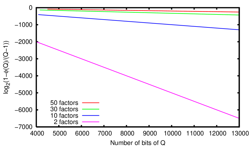
Figure 1: Actual probability of failure of Algorithm 1 with $L=2^{20}$

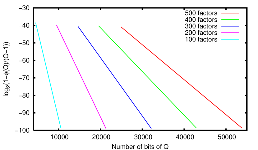
Figure 2: Actual probability of failure for $Q$ with many distinct factors

the experimental data then shows that in practice no probability less than $1-2^{-40}$ is possible even with $L$ as small as $2^{20}$.
Provided that one is ready to accept a fixed probability, further improvements on the asymptotic complexity can be made. Indeed, D. Knuth said ”For the probability less than $(\frac{1}{4})^{25}$ that such a 25-times-in-row procedures gives the wrong information about n. It’s much more likely that our computer has dropped a bit in its calculations, due to hardware malfunctions or cosmic radiations, than that algorithm P has repeatedly guessed wrong.” We thus provide a version of our algorithm guaranteeing that the probability of incorrect answer is lower than $2^{-40}$:

Algorithm 3: If $p$ is small ($p<45171967$), factor $p-1$ completely, otherwise apply Algorithm 1 with $B=log^{5.298514}{p}$.

With Pollard’s rho factoring, the average asymptotic bit complexity is then $O(\log^{4.649257}{p})$: Factoring numbers lower than $45171967$, takes constant time. Now for larger primes and $B=\log^{\alpha}(p)$, we just remark that $(1+\frac{2}{p-1})(1-\frac{1}{B})^{\log_{B}{\frac{p-1}{2}}}$ is increasing in $p$, so that it is bounded by its first value. Numerical approximation of $\alpha$ so that the latter is $1-2^{-40}$ gives $5.298514$. The complexity exponent follows as it is $2+\frac{\alpha}{2}$. One can also apply the same arguments e.g. for a probability $1-2^{-55}$ and factoring all primes $p<2^{512}$ (since $513$-bit numbers are nowadays factorizable), then slightly degrading the complexity to $O(log^{5.229921}{p})$. We have thus proved that a probability of at least $1-2^{-40}$ can always be guaranteed. In other words, our algorithm is able to efficiently produce “industrial-strength” primitive roots.

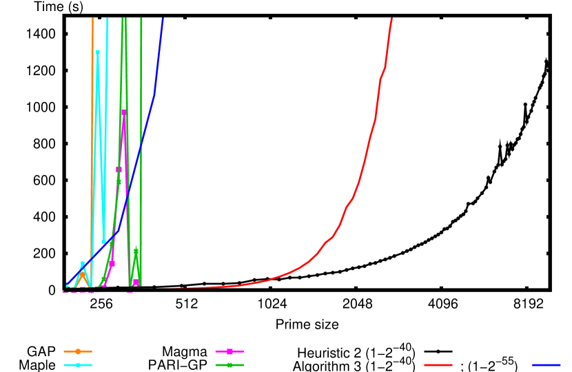
Figure 3: Generations of primitive roots

This is for instance illustrated when comparing our algorithm, implemented in C++ with GMP, to existing software (Maple 9.5, Pari-GP, GAP 4r4 and Magma 2.11) on an Intel PIV 2.4GHz. This comparison is shown on figure 3. Of course, the comparison is not fair as other softwares are always factoring $p-1$ completely. Still we can see the progress in primitive root generation that our algorithm has enabled.

5 Analysis of the algorithm for composite numbers

In this section we propose an analysis of the behavior of the algorithm for composite numbers. Indeed, our algorithm can also be used to produce high, if not maximal, order element modulo a composite number. This analysis is also used section 6.2 for the probabilistic primality test. It is well known that there exists primitive roots for every number of the form $2$, $4$, $p^{k}$ or $2p^{k}$ with $p$ an odd prime. On the other hand, Euler’s theorem states that every invertible $a\in\leavevmode\kern 1.00006pt\raise 0.0pt\hbox{$\mathbb{Z}$}\kern-1.00006pt/\kern-1.49994pt\lower 1.29167pt\hbox{$p$}\mbox{$\mathbb{Z}$}^{*}$ satisfies $a^{\varphi(n)}\equiv 1[n]$. Thus, for composite numbers $n$ not possessing primitive roots, $\varphi(n)$ is not a possible order of an invertible. We therefore use $\lambda(m)$, Carmichael’s lambda function, the maximal order of an invertible element in the multiplicative group ($\leavevmode\kern 1.00006pt\raise 0.0pt\hbox{$\mathbb{Z}$}\kern-1.00006pt/\kern-1.49994pt\lower 1.29167pt\hbox{$p$}\mbox{$\mathbb{Z}$}^{*}$, $\times$). See e.g. [16, 10, 3], for more details. Of course, $\lambda$ and $\varphi$ coincide for $2$, $4$, $p^{k}$ and $2p^{k}$, for $p$ and odd prime. Then $\lambda(2^{e})=2^{e-2}$ for $e\geq 3$. Now, for the other cases, since $\varphi\left(\prod p_{i}^{k_{i}}\right)=\prod(p_{i}-1)p_{i}^{k_{i}-1}$ for distinct primes $p_{i}$, we obtain this similar formula for $\lambda$: $\lambda\left(\prod p_{i}^{k_{i}}\right)=lcm\{\lambda(p_{i}^{k_{i}})\}$. Eventually, we also obtain this corollary of Euler’s theorem:

Corollary 4

Every invertible $a$ within $\leavevmode\kern 1.00006pt\raise 0.0pt\hbox{$\mathbb{Z}$}\kern-1.00006pt/\kern-1.49994pt\lower 1.29167pt\hbox{$p$}\mbox{$\mathbb{Z}$}^{*}$ satisfies $a^{\lambda(n)}\equiv 1[n]$.

Proof. $n=\prod p_{i}^{e_{i}}$ for distinct primes $p_{i}$. Then $\varphi(p_{i}^{e_{i}})$ divides $\lambda(n)$. This, together with Euler’s theorem shows that $a^{\lambda(n)}\equiv 1[p_{i}^{e_{i}}]$. The Chinese theorem thus implies that the latter is also true modulo the product of the $p_{i}^{e_{i}}$. $\Box$ This corollary shows that the order of any invertible must divide $\lambda(n)$. For $n$ prime, the number of invertibles having order $d|n-1$ is exactly $\varphi(d)$ so that $\sum_{d|k}\varphi(d)=k$ for $k|n-1$. We have the following analogue for $n$ a composite number:

Proposition 5

The number of invertibles having order $d|\lambda(n)$ is $\sum_{S_{d}}\prod_{j=1}^{\omega}\varphi(d_{j})$ for $n=p_{1}^{e_{1}}\ldots p_{\omega}^{e_{\omega}}$ and $S_{d}=\{(d_{1},\ldots,d_{\omega})$ s.t. $d_{j}|\varphi(p_{j}^{e_{j}})$ and $lcm\{d_{j}\}=d\}$.

Proof. By the Chinese theorem, an element has order $d$ if and only if the lcm of its orders modulo the $p_{j}^{e_{j}}$ is $d$. Then there are exactly $\varphi(d_{j})$ elements of order $d_{j}$ modulo $p_{j}^{e_{j}}$. $\Box$

Let us have a look of this behavior on an example: let $n=45$ so that $\varphi(45)=6\times 4=24$ and $\lambda(45)=12$. We thus know that any order modulo $9$ divides $\varphi(9)=6$ and that any order modulo $5$ divides $\varphi(5)=4$. This gives the different orders of the $24$ invertibles shown on table 1.

order			# of elements of that
modulo 45	modulo 9	modulo 5	order modulo 45
1	1	1	1
	1	2	1
	2	1	1
	2	2	1
2			3
3	3	1	$\varphi(3)\times\varphi(1)=$ 2
	1	4	$\varphi(1)\times\varphi(4)=2$
	2	4	$\varphi(2)\times\varphi(4)=2$
4			4
	6	1	$\varphi(6)\times\varphi(1)=2$
	3	2	$\varphi(3)\times\varphi(2)=2$
	6	2	$\varphi(6)\times\varphi(2)=2$
6			6
	3	4	$\varphi(3)\times\varphi(4)=4$
	6	4	$\varphi(6)\times\varphi(4)=4$
12			8

Table 1: Elements of a given order modulo 45

It would be highly desirable to have tight bounds on those number of elements of a given order. Moreover, these bounds should be easily computable (e.g. not requiring some factorization !). In [5, 19], the following is proposed:

Proposition 6

[5, Corollary 6.8] For $n$ odd, the number of elements of order $\lambda(n)$ (primitive $\lambda-$roots) is larger than $\varphi(\varphi(n))$.

Now, this last result shows that actually quite a lot of elements are of maximal order modulo $n$. Using this fact, a modification of algorithm $1$ can then produce with high probability an element of maximal order even though $n$ is composite.

6 Applications

Of course, our generation can be applied to any application requiring the use of primitive roots. In this section we show the speed of our method compared to generation of primes with known factorization and propose a generalization of Miller-Rabin probabilistic primality test and of Davenport’s strengthenings [7].

6.1 Faster pseudo random generators construction or key exchange

The use of a generator and a big prime is the core of many cryptographic protocols. Among them are Blum-Micali pseudo-random generators [4], Diffie-Hellman key exchange [8], etc.
In this section we just compare the generation of primes with known factorization [1], so that primitive roots of primes with any given size are computable. The idea in [4] is to iteratively and randomly build primes so that the factorizations of $p_{i}-1$ are known. For cryptanalysis reasons their original method selects the primes and primitive roots bit by bit and is therefore quite slow. On figure 4 we then present also a third way, which is to generate the prime with known factorization as in [1], but then to generate the primitive root deterministically with our algorithm (since the factorization of $p-1$ is known). We compare this method with the following full-probabilistic way:

1. By trial and error generate a probable prime (e.g. a prime passing several Miller-Rabin tests [18]).

2. Generate a probable primitive root by Heuristic 2.

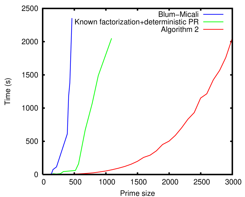
Figure 4: Blum-Micali primes with known factorization vs Industrial-strength primitive roots

We see on figure 4 that our method is faster and allows for the use of bigger primes/generators.

6.2 Probabilistic Lucas primality test

The deterministic primality test of Lucas is actually the existence of primitive roots:

Theorem 7 (Lucas)

Let $p>0$. If one can find an $a>0$ such that $a^{p-1}\equiv 1\,mod\,p$ and $a^{\frac{p-1}{q}}\operatorname{\mskip 4.0mu\not\equiv\mskip 4.0mu}1\,mod\,p$, as soon as $q$ divides $p-1$, then $p$ is prime.

We propose here as a probabilistic primality test to try to build a primitive root. If one succeeds then the number is prime with high probability else it is either proven composite or composite with a high probability.
Now for the complexity, we do not pretend to challenge Miller-Rabin test for speed ! Well, one often needs to perform several Miller-Rabin tests with distinct witnesses, so that the probability of being prime increases. Our idea is the following: since one tests several witnesses, why not use them as factors of our probable primitive root ! This idea can then be viewed as a generalization of Miller-Rabin: we not only test for orders of the form $\frac{n-1}{2^{e}}$ but also for each order of the form $\frac{n-1}{q^{e}}$ where $q$ is a small prime factor of $n-1$. The effective complexity (save maybe from the partial factorization) will not suffer and the probability can jump as soon as an element with very high order is generated. The algorithm is then a slight modification of algorithm 1, where we let $F(B,Q)=1-(1+\frac{1}{Q-1})(1-\frac{1}{B})^{\log_{B}{Q}}$:

Input: $n\geq 3$, odd.

Input: A failure probability $0<\epsilon<1$.

Output: Whether $n$ is prime and a certificate of primality,

Output: or $n$ is composite and a factor (or just a Fermat witness),

Output: or $n$ is prime with probability of error less than $\epsilon$,

Output: or $n$ is composite with probability of error less than $\epsilon$.

begin  Set $P=1$, $a=1$, $Q=n-1$ and $q=2$.

while $Q>n^{\frac{2}{3}}$ do  Randomly choose $\alpha\mod n$.

if $gcd(\alpha,n)\neq 1$ or $gcd(\alpha^{\frac{n-1}{q}}-1,n)\notin\{1;n\}$ or $\alpha^{n-1}\operatorname{\mskip 4.0mu\not\equiv\mskip 4.0mu}1[n]$ or $(q==2$ and $n~{}\text{is not a strong pseudoprime to the base}~{}\alpha)$ then  return $n$ is composite.   else if $\alpha^{\frac{n-1}{q}}\equiv 1\;mod\;n$ then  Set $P=P/q$.

if $P\leq\epsilon$ then  return $n$ is probably composite with error less than $P$.    else  - Set $e$ to the greatest power of $q$ dividing $Q$.

- Set $Q=Q/q^{e}$.

- Set $a=a\times\alpha^{\frac{n-1}{q^{e}}}$.

- Set $k=k\cup\{q^{e}\}$.

- Refine $B$ such that $F(B,Q)==4\epsilon$.

- Find a new prime factor $q$ of $Q$ with $q<B$, otherwise set $q=Q$.     if Every $q$ was prime then  return $n$ is prime and $(a,k)$ is a certificate. else  return $n$ is probably prime with error less than $F(B,q)$.   end

Algorithm 2 Probabilistic Lucas primality test

Remark 8

The exponentiations by $\frac{n-1}{q}$ can in practice be factorized in a “Lucas-tree” [22, 6].

Remark 9

Algorithm 2 is correct for the primes and most of the composite numbers.

Proof. Correctness for prime numbers is the correctness of the pseudo primitive root generation.
Now for composite numbers: the idea is that first of all, only Carmichael numbers will be able to pass the pseudo prime test several times.
The $4\epsilon$ then follows since at least one $\alpha$ passed the strong pseudoprime test. This reduces the possible Carmichael numbers able to pass our test. Then, for most of the Carmichael numbers, $\lambda(n)$ divides $n-1$ but, moreover, $\lambda(n)$ also divides $\frac{n-1}{q}$ for some $q$, factor of $n-1$. Therefore, $\alpha^{\frac{n-1}{q}}$ will always be one. If $n$ is prime on the contrary, only $\frac{1}{q}$ elements will have order a multiple of $q$.
Now for the $n^{\frac{2}{3}}$ in the loop. The argument is the same as for the Pocklington theorem [6, Theorem 4.1.4] and the Brillhart, Lehmer and Selfridge theorem [6, Theorem 4.1.5]: let $n-1=kQ$ and let $p$ be a prime factor of $n$. The algorithm has found an $a$ verifying $a^{n-1}\equiv 1\mod n$. Hence, the order of $a^{Q}\mod p$ is a divisor of $\frac{n-1}{Q}=k$. Now, since $gcd(a^{\frac{n-1}{q}}-1,n)=1$ for each prime $q$ dividing $k$, this order is not a proper divisor of $k$, so is equal to $k$. Hence, $k$ must be a divisor of $p-1=\varphi(p)$. We conclude that each prime factor of $n$ must exceed $k$. From this, Pocklington’s theorem states that if $k$ is greater than $\sqrt{n}$, $n$ is prime. And then, Brillhart-Lehmer-Selfridge theorem states that if $k$ is in between $n^{\frac{1}{3}}$ and $n^{\frac{1}{2}}$ then $n$ must be prime or composite with exactly two prime factors [6, Theorem 4.1.5]. But $n$ has escaped our previous tests only if $n$ is a Carmichael number. Fortunately, Carmichael numbers must have at least $3$ factors [17, Proposition V.1.3]. Now, whenever $Q$ is below $n^{\frac{2}{3}}$, $k$ exceeds $n^{\frac{1}{3}}$ and then $n$ must be prime otherwise $n$ would have more than $3$ factors each of those being greater than $n^{\frac{1}{3}}$. $\Box$

Here is an example of Carmichael number, $1729$. $1728=2^{6}3^{3}$, where $\lambda(1729)=2^{2}3^{2}$. Then $\frac{n-1}{q}$ is either $864$ or $576$ both of which are divisible by $36=\lambda(1729)$. Therefore, our test will detect $1729$ to be probably composite with any probability of correctness. Figure 5 shows that this algorithm is highly competitive with repeated applications of GMP’s strong pseudo prime test (i.e. with the same estimated probability of correctness). Depending on the success of the partial factorization, our test can even be faster (timing, on a PIV 2.4GHz, presented on figure 5 are the mean time between 4 distinct runs).

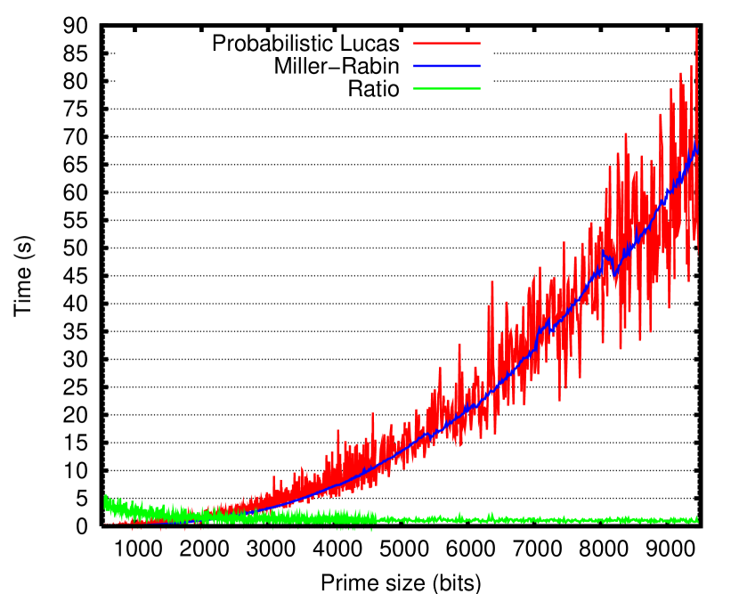
Figure 5: Probabilistic Lucas vs GMP’s Miller-Rabin for primes with probability $<10^{-6}$

Haplessly, some Carmichael numbers will still pass our test. The following results, sharpening [11, lemma 1], explains why:

Theorem 10

Let $n=p_{1}^{e_{1}}\ldots p_{\omega}^{e_{\omega}}$. Let $q$ be a prime divisor of $\varphi(n)$, and $(f_{1},\ldots,f_{\omega})$ be the maximal values for which $q^{f_{i}}$ divides $\varphi(p_{i}^{e_{i}})$. There are

$$\varphi(n)\left(1-\frac{1}{q^{\sum f_{i}}}\right)$$

invertible elements of order divisible by $q$ (i.e. for which $\alpha^{\frac{\lambda(n)}{q}}\operatorname{\mskip 4.0mu\not\equiv\mskip 4.0mu}1\mod n$).

Proof. By the Chinese remainder theorem, one can consider the moduli by $p_{i}^{e_{i}}$ separately. Suppose, without loss of generality, that $p_{1}^{e_{1}}$ is such that $f_{1}>0$. Otherwise all the $f_{i}$ are $0$ and the theorem is still correct. Consider a generator $g$ of the invertibles modulo $p_{1}^{e_{1}}$. An element has $q$ in its order if and only if its index with respect to $g$ contains $q^{f_{1}}$. There are exactly $1-\frac{1}{q^{f_{1}}}$ such elements among the elements of $\leavevmode\kern 1.00006pt\raise 0.0pt\hbox{$\mathbb{Z}$}\kern-1.00006pt/\kern-1.49994pt\lower 1.29167pt\hbox{$p_{1}^{e_{1}}$}\mbox{$\mathbb{Z}$}$. By the Chinese theorem, among the elements having their order divisible by $q$ modulo $n$, we have then identified $\varphi(n)(1-\frac{1}{q^{f_{1}}})$ of them: the ones having their order modulo $p_{1}^{e_{1}}$ divisible by $q$. Now the others are among the $\varphi(n)(\frac{1}{q^{f_{1}}})$ that remains. Just now consider those modulo $p_{2}^{e_{2}}$. If $f_{2}==0$ then we have not found any new element. Otherwise, $1-\frac{1}{q^{f_{2}}}$ of them are of order divisible by $q$. Well, actually, in both cases, we can state that $1-\frac{1}{q^{f_{2}}}$ of them are of order divisible by $q$. We have thus found some other elements: $\varphi(n)(\frac{1}{q^{f_{1}}})(1-\frac{1}{q^{f_{2}}})$. This added to the previously found elements makes $\varphi(n)(1-\frac{1}{q^{f_{1}}q^{f_{2}}})$. Doing such a counting for each of the remaining $p_{i}^{e_{i}}$ gives the announced formula. $\Box$

For instance, take a Carmichael number still passing our test whenever $B~{}\leq~{}1450$: $37690903213=229\times 2243\times 73379$. Well, $37690903212=19\times 2^{2}\times 3\times 59\times 1451\times 1931$ and $\lambda(37690903213)=19\times 2^{2}\times 3\times 59\times 1931$. Then, $Q$ will be $1451\times 1931$ and our algorithm will be able to find elements for which $\alpha^{\frac{n-1}{Q}}\operatorname{\mskip 4.0mu\not\equiv\mskip 4.0mu}1\mod n$: those of which order is divisible by $1931$. Unfortunately, there are quite a lot of them: $\varphi(n)\frac{1930}{1931}=37489647840\approx(1-.00533962722683134975)n$. Thus, there are more than 5 chances over a thousand to choose an element $\alpha$ for which $\alpha^{\frac{n-1}{1451\times 1931}}\operatorname{\mskip 4.0mu\not\equiv\mskip 4.0mu}1\mod n$. Even though this is much higher than $\frac{1}{Q}$ (if $n$ was prime), this probability will not be detected abnormal by our algorithm. Now, even if $p-1$ is seldom smooth for $p$ prime [21], one can wonder if this is still the case for this special kind of Carmichael numbers $\ldots$

7 Conclusion

We provide here a new very fast and efficient algorithm generating primitive roots. On the one hand, the algorithm has a polynomial time bit complexity when all existing algorithms where exponential. This is for instance illustrated when comparing it to existing software on figure 3. On the other hand, our algorithm is probabilistic in the sense that the answer might not be a primitive root. We have seen in this paper however, that the chances that an incorrect answer is given are less important than say “hardware malfunctions”. For this reason, we call our answers “Industrial-strength” primitive roots.

Then, we propose a new probabilistic primality test using this primitive root generation. This test can be viewed as a generalization of Miller-Rabin’s test to other small prime factors dividing $n-1$ The test is then quantifying the information gained by finding elements of large order modulo $n$. When a given probability of correctness is desirable for the test, our algorithm is heuristically competitive with repeated applications of Miller-Rabin’s.

References

- [1] Eric Bach. How to generate factored random numbers. SIAM Journal on Computing, 17(2):179–193, April 1988. Special issue on cryptography.
- [2] Eric Bach. Comments on search procedures for primitive roots. Mathematics of Computation, 66(220):1719–1727, October 1997.
- [3] Eric Bach and Jeffrey Shallit. Algorithmic Number Theory: Efficient Algorithms. MIT press, 1996.
- [4] Manuel Blum and Silvio Micali. How to generate cryptographically strong sequences of pseudo-random bits. SIAM Journal on Computing, 13(4):850–864, November 1984.
- [5] Peter J. Cameron and D. A. Preece. Notes on primitive roots, March 2003. http://www.maths.qmul.ac.uk/~pjc/csgnotes/lambda.pdf.
- [6] Richard Crandall and Carl Pomerance. Prime Numbers, a computational perspective. Springer, 2001.
- [7] J. H. Davenport. Primality testing revisited. In Paul S. Wang, editor, Proceedings of ISSAC ’92. International Symposium on Symbolic and Algebraic Computation, pages 123–129, New York, NY 10036, USA, 1992. ACM Press.
- [8] Whitfield Diffie and Martin E. Hellman. New directions in cryptography. IEEE Transactions on Information Theory, IT-22(6):644–654, 1976.
- [9] Peter D. T. A. Elliott and Leo Murata. On the average of the least primitive root modulo p. Journal of The london Mathematical Society, 56(2):435–454, 1997.
- [10] Paul Erdös, Carl Pomerance, and Eric Schmutz. Carmichael’s lambda function. Acta Arithmetica, 58:363–385, 1991.
- [11] John B. Friedlander, Carl Pomerance, and Igor Shparlinski. Period of the power generator and small values of Carmichael’s function. Mathematics of Computation, 70(236):1591–1605, October 2001. See corrigendum [12].
- [12] John B. Friedlander, Carl Pomerance, and Igor Shparlinski. Corrigendum to “Period of the power generator and small values of Carmichael’s function”. Mathematics of Computation, 71(240):1803–1806, October 2002. See [11].
- [13] Joachim von zur Gathen and Igor Shparlinski. Orders of Gauss periods in finite fields. Applicable Algebra in Engineering, Communication and Computing, 9:15–24, 1998.
- [14] Godfrey Harold Hardy and E. Maitland Wright. An Introduction to the Theory of Numbers. Oxford University Press, fifth edition, 1979.
- [15] Toshiya Itoh and Shigeo Tsujii. How to generate a primitive root modulo a prime. Technical Report 009-002, IPSJ SIGNotes ALgorithms Abstract, 2001.
- [16] Donald E. Knuth. Seminumerical Algorithms, volume 2 of The Art of Computer Programming. Addison-Wesley, Reading, MA, USA, edition, 1997.
- [17] Neal Koblitz. A course in number theory and cryptography, volume 114 of Graduate texts in mathematics. Springer-Verlag, Berlin, Germany / Heidelberg, Germany / London, UK /, etc., 1987.
- [18] Gary L. Miller. Riemann’s hypothesis and tests for primality. In Conference Record of Seventh Annual ACM Symposium on Theory of Computation, pages 234–239, Albuquerque, New Mexico, May 1975.
- [19] Thomas W. Müller and Jan-Christof Schlage-Puchta. On the number of primitive roots. Acta Arithmetica, 115(3):217–223, 2004.
- [20] T. J. O’Gorman, J. M. Ross, A. H. Taber, J. F. Ziegler, H. P. Muhlfeld, C. J. Montrose, H. W. Curtis, and J. L. Walsh. Field testing for cosmic ray soft errors in semiconductor memories. IBM Journal of Research and Development, 40(1):41–50, January 1996.
- [21] Carl Pomerance and Igor E. Shparlinski. Smooth orders and cryptographic applications. Lecture Notes in Computer Science, 2369:338–348, 2002. ANTS-V: 5th International Algorithmic Number Theory Symposium.
- [22] Vaughan R. Pratt. Every prime has a succinct certificate. SIAM Journal on Computing, 4(3):214–220, 1975.
- [23] Guy Robin. Estimation de la fonction de Tchebycheff sur le k-ième nombre premier et grandes valeurs de la fonction nombre de diviseurs premiers de . Acta Arithmetica, XLII:367–389, 1983.
- [24] Victor Shoup. Searching for primitive roots in finite fields. Mathematics of Computation, 58(197):369–380, January 1992.
- [25] Samuel S. Wagstaff, Jr. Cryptanalysis of number theoretic ciphers. Chapman-Hall / CRC, 2003.