Measurements of $B\rightarrow D_{s}^{(*)+}D^{*(*)}$ Branching Fractions

Abstract

This article describes improved measurements by CLEO of the $B^{0}\rightarrow D_{s}^{+}D^{*-}$ and $B^{0}\rightarrow D_{s}^{*+}D^{*-}$ branching fractions, and first evidence for the decay $B^{+}\rightarrow D_{s}^{(*)+}\bar{D}^{**0}$, where $\bar{D}^{**0}$ represents the sum of the $\bar{D}_{1}(2420)^{0}$, $\bar{D}_{2}^{*}(2460)^{0}$, and $\bar{D}_{1}(j=1/2)^{0}$ $L=1$ charm meson states. Also reported is the first measurement of the $D_{s}^{*+}$ polarization in the decay $B^{0}\rightarrow D_{s}^{*+}D^{*-}$. A partial reconstruction technique, employing only the fully reconstructed $D_{s}^{+}$ and slow pion $\pi_{s}^{-}$ from the $D^{*-}\rightarrow\bar{D}^{0}\pi^{-}_{s}$ decay, enhances sensitivity. The observed branching fractions are ${\mathcal{B}}(B^{0}\rightarrow D_{s}^{+}D^{*-})=(1.10\pm 0.18\pm 0.10\pm 0.28)\%$ , ${\mathcal{B}}(B^{0}\rightarrow D_{s}^{*+}D^{*-})=(1.82\pm 0.37\pm 0.24\pm 0.46)\%$ , and ${\mathcal{B}}(B^{+}\rightarrow D_{s}^{(*)+}\bar{D}^{**0})=(2.73\pm 0.78\pm 0.48\pm 0.68)\%$, where the first error is statistical, the second systematic, and the third is the uncertainty in the $D_{s}^{+}\rightarrow\phi\pi^{+}$ branching fraction. The measured $D_{s}^{*+}$ longitudinal polarization, $\Gamma_{L}/\Gamma=(50.6\pm 13.9\pm 3.6)\%$, is consistent with the factorization prediction of 54%.

I Introduction

Measurements of weak decays of $B$ mesons are fundamental to testing and understanding the standard model. Previous measurements of the inclusive $B\rightarrow D_{s}^{+}X$ branching fraction report a value of $(12.1\pm 1.0\pm 3.0)\%$. The first error is the combined statistical and systematic uncertainties, and the second is due to the uncertainty in the $D_{s}^{+}\rightarrow\phi\pi^{+}$ branching fraction. This is significantly larger than the sum of $D_{s}^{+}$ production from exclusive $b\rightarrow c\bar{c}s$ modes observed to date[1]. These exclusive modes, of the form $B\rightarrow D_{s}^{+}D$, $B\rightarrow D_{s}^{*+}D$, $B\rightarrow D_{s}^{+}D^{*}$, and $B\rightarrow D_{s}^{*+}D^{*}$, sum to $(6.6\pm 1.3\pm 1.7)\%$ for the $B^{+}$ case and $(4.8\pm 1.0\pm 1.2)\%$ for the $B^{0}$. This yields a deficit of $(5.5\pm 1.6)\%$ for the $B^{+}$ and $(7.3\pm 1.4)\%$ for the $B^{0}$, where the $D_{s}^{+}\rightarrow\phi\pi^{+}$ branching fraction uncertainty does not affect this difference[1]. This article reports new measurements of $B\rightarrow D_{s}^{(*)+}D^{*(*)}$ decays from CLEO. First evidence is offered for the decay $B^{+}\rightarrow D_{s}^{(*)+}\bar{D}^{**0}$, where $\bar{D}^{**0}$ denotes the sum of the $\bar{D}_{1}(2420)^{0}$, $\bar{D}_{2}^{*}(2460)^{0}$, and $\bar{D}_{1}(j=1/2)^{0}$ $L=1$ charm meson states. This decay mode may bridge a substantial portion of the inclusive and exclusive rate difference. Also reported are improved measurements of the modes $B^{0}\rightarrow D_{s}^{+}D^{*-}$ and $B^{0}\rightarrow D_{s}^{*+}D^{*-}$. These decays occur predominantly via the spectator diagram of Figure 1; the $W^{+}$ decays into a $D_{s}^{+}$ or $D_{s}^{*+}$ meson, and the charm anti-quark and spectator quark hadronize as either a $D^{*}$ or $D^{**}$ meson.

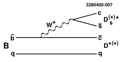
FIG. 1.: The spectator diagram for $B\rightarrow D_{s}^{(*)+}D^{*(*)}$ decay.

Additionally, this Article presents the first measurement of $D_{s}^{*+}$ polarization for the mode $B^{0}\rightarrow D_{s}^{*+}D^{*-}$, providing an effective test of the factorization assumption in $B\rightarrow D^{*-}X$ decays with high $q^{2}$, where $q^{2}=M_{X}^{2}$, and $X$ is a vector meson. Factorization assumes the lack of final state interactions between the products of hadronic $B$ decays, and has successfully predicted the vector-vector polarization of the low $q^{2}$ mode $B\rightarrow D^{*-}\rho$[2, 3, 4, 5, 6]. It is possible that the factorization assumption of no final state interactions may be simplistic and inapplicable to modes of higher $q^{2}$ such as $B^{0}\rightarrow D_{s}^{*+}D^{*-}$; however, the results presented here are consistent with the factorization prediction.

Previous measurements of $B^{0}\rightarrow D_{s}^{+}D^{*-}$ and $B^{0}\rightarrow D_{s}^{*+}D^{*-}$ at CLEO and ARGUS made use of the full reconstruction technique[1][7], which requires reconstruction of all particles in the final state. The most recent CLEO results using full reconstruction reported relatively small event yields of $18.4\pm 4.5$ and $17.7\pm 4.4$ in the $D_{s}^{+}D^{*-}$ and $D_{s}^{*+}D^{*-}$ channels, respectively. Following these, a partial reconstruction technique was developed that required only some of the $B^{0}\rightarrow D_{s}^{*+}D^{*-}$ final state particles, reporting an increased sample size of $76\pm 11$ events[8].

This analysis employs a more refined partial reconstruction technique, using only the $D_{s}^{+}$ and the soft pion $\pi_{s}^{-}$ from the $D^{*-}\rightarrow\bar{D}^{0}\pi_{s}^{-}$ decay, thereby increasing the statistics over full reconstruction by a factor between five and eight, depending on mode. The analysis is sensitive to any $B\rightarrow D_{s}^{+}D^{*-}X$ final state, such as $B\rightarrow D_{s}^{(*)+}D^{**}$, when $D^{**}\rightarrow D^{*-}\pi$. The method is based on techniques developed by CLEO for improved measurement of $D_{s}^{+}\rightarrow\phi\pi^{+}$[8] and $B\rightarrow D^{*}\pi$[9].

After a short description of the detector and the criteria used for selecting charged particle candidates in Section II, the $D_{s}^{+}$ and $\pi_{s}^{-}$ reconstruction is described in Section III. In Section IV the partial reconstruction technique is developed for separating the combined $D_{s}^{(*)}D^{*(*)}$ signal from background. Once the background levels have been determined, in Section V a two-dimensional parameter space is defined and used to separate the individual $D_{s}D^{*}$, $D_{s}^{*}D^{*}$, and $D_{s}^{(*)}D^{**}$ signals, followed by a review of systematic errors in Section VI. The polarization of $D_{s}^{*}D^{*}$ production is measured and compared with the factorization prediction in Section VII, and the results summarized and discussed in the final section.

II EVENT SELECTION

The data used in this analysis were collected at the Cornell Electron Storage Ring (CESR) between 1990 and 1995, and consist of hadronic events produced in $e^{+}e^{-}$ annihilations. The integrated luminosity of this data sample is $3.14\pm 0.06$ ${\rm fb^{-1}}$ collected at the $\Upsilon(4S)$ resonance (referred to as on-resonance data), and $1.69\pm 0.03$ ${\rm fb^{-1}}$ from a center-of-mass energy just below the threshold for producing $B\bar{B}$ mesons (referred to as off-resonance or continuum data). The on-resonance data corresponds to $(3.36\pm 0.06)\times 10^{6}$ $B\bar{B}$ pairs.

The CLEO II detector is used to measure both neutral and charged particles with excellent resolution and efficiency[10]. Hadronic events are selected by requiring a minimum of three charged tracks, a total visible energy greater than 15% of the center-of-mass energy (this reduces contamination from two-photon interactions and beam-gas events), and a primary vertex within $\pm 5$ cm in the $z$ direction and $\pm 2$ cm in the $r$-$\phi$ plane of the beam centroid.

Charged tracks are required to be of good quality and consistent with the primary vertex in both the $r$-$\phi$ and $r$-$z$ planes. Tracks must also have $dE/dx$ and time-of-flight information consistent with their pion or kaon hypotheses, when such information exists and is of good quality.

Apart from the visible energy criterion, neutral particles were not used in this analysis.

A geant[11] based Monte Carlo simulation was used to generate large samples of the individual $D_{s}^{(*)}D^{*(*)}$ signal modes from $\Upsilon(4S)\rightarrow B\bar{B}$ decays, and model their interactions with the CLEO detector. These samples were then processed in the same manner as the data. Further discussion of the simulation is given in the treatment of systematic errors.

III $D^{+}_{s}$ AND SLOW $\pi^{-}_{s}$ RECONSTRUCTION

The $D_{s}^{+}$ is reconstructed through the $D_{s}^{+}\rightarrow\phi\pi^{+}$, $\phi\rightarrow K^{+}K^{-}$ decay channel, which has a signal-to-background ratio nearly two times higher than the next cleanest $D_{s}^{+}$ decay mode[8]. Fast $\pi^{+}$/$K^{+}$ tracks ($p\geq 200\ {\rm MeV}/c$) must originate within $\pm 5$ cm in the $z$ direction and $\pm 5$ mm in the $r$-$\phi$ plane of the beam centroid. For slow $\pi^{+}$/$K^{+}$ tracks ($p\leq 200\ {\rm MeV}/c$) the $z$ requirement is loosened to within $\pm 20$ cm. The $K^{+}K^{-}$ invariant mass is required to be within 9 MeV of the $\phi$ mass. Two angles are used in suppressing background. The first is the $D_{s}^{+}$ decay angle $\theta_{D}$, which is the angle between the $\phi$ direction in the $D_{s}^{+}$ rest frame and the $D_{s}^{+}$ boost direction. Requiring $\cos{\theta_{D}}\leq 0.80$ eliminates a large combinatoric background peak near $\cos{\theta_{D}}=1$ resulting from the numerous low momentum pions, while the signal is constant in $\cos{\theta_{D}}$. The second angle is $\theta_{H}$, the $\phi$ decay angle between the $K^{+}$ and $D_{s}^{+}$ direction in the $\phi$ rest frame. Due to the $\phi$ helicity the signal follows a $\cos^{2}{\theta_{H}}$ distribution while the background is constant in $\cos{\theta_{H}}$. Requiring $|\cos{\theta_{H}}|\geq 0.35$ removes 35% of the background and retains 96% of signal. The resulting $\phi\pi^{+}$ invariant mass spectrum is shown in Figure 2, and the $\phi\pi^{+}$ mass is then required to be within 12 MeV of the $D_{s}^{+}$ mass. Finally, the kinematics of $B\rightarrow D_{s}^{(*)+}D^{**}$ decays constrain the magnitude of $D_{s}^{+}$ momentum to between 1250 MeV/$c$ and 1925 MeV/$c$, and these requirements are imposed here.

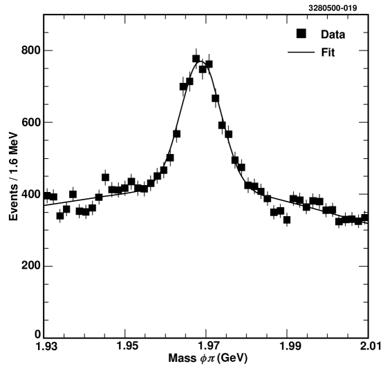
FIG. 2.: The $\phi\pi^{+}$ mass spectrum for the on-resonance data. The $\phi\pi^{+}$ mass is further required to be within 12 MeV of the $D_{s}^{+}$ mass.

The slow pion $\pi^{-}_{s}$ from the $D^{*-}$ must have charge opposite to the $D_{s}^{+}$ and originate within $\pm 5$ mm in the $r$-$\phi$ plane of the primary vertex. No $z$ requirement is placed on the $\pi^{-}_{s}$, but it must have a momentum greater than 50 MeV/$c$ and less than 210 MeV/$c$.

IV SEPARATION OF $D_{s}^{(*)+}D^{*(*)}$ SIGNAL FROM BACKGROUND

A Two-Body $B$ decays to $D_{s}^{+}D^{*-}$ Final States

At the CLEO II experiment, $e^{+}e^{-}$ collisions can create an $\Upsilon(4S)$ resonance, which decays to a pair of $B$ mesons. The $B$’s are produced nearly at rest ($\beta=0.0646$) and, for the decay chain $\Upsilon(4S)\rightarrow B^{0}\bar{B}^{0}$, $B^{0}\rightarrow D_{s}^{+}D^{*-}$, and $D^{*-}\rightarrow\bar{D^{0}}\pi_{s}^{-}$, the $D_{s}^{+}$ and soft pion $\pi^{-}_{s}$ are nearly back-to-back in the lab frame because of the small $5.83\pm 0.03$ MeV energy release in the $D^{*-}\rightarrow\bar{D^{0}}\pi_{s}^{-}$ transition. By making use of their relative direction, as well as the beam energy and kinematic constraints of the decay, the $D_{s}^{+}$ and the $\pi_{s}^{-}$ allow reconstruction of the $D_{s}^{+}D^{*-}$ final state.

Other two-body $B$ decays leading to $D_{s}^{+}D^{*-}$ final states, with strong $(D_{s}^{+},\pi_{s}^{-})$ correlations, are summarized in Table I. These are modes producing a $D_{s}^{*+}$ that decays to $D_{s}^{+}\gamma$ or $D_{s}^{+}\pi^{0}$, or producing a $D^{**}$ that decays to $D^{*-}\pi$. It should be noted that this method is not sensitive to $B\rightarrow D_{s}^{**}D^{*-}$, as the $D_{s}^{**}$ decays predominantly to $DK$ and no $D_{s}^{**}\rightarrow D_{s}X$ decays have been observed[12]. Other relevant modes, such as three-body $B$ decays of the form $B\rightarrow D_{s}^{(*)+}D^{*-}\pi$, are treated in the discussion of systematic errors.

TABLE I.: $D_{s}^{+}D^{*-}$ final states from two-body $B$ decays.

$B^{0}$ Decays	$B^{+}$ Decays
$B^{0}\rightarrow D_{s}^{+}D^{*-}$
$B^{0}\rightarrow D_{s}^{*+}D^{*-}$
(where $D_{s}^{*+}\rightarrow$
$D_{s}^{+}\gamma$ / $D_{s}^{+}\pi^{0}$)
$B^{0}\rightarrow D_{s}^{+}D^{**-}$	$B^{+}\rightarrow D_{s}^{+}\bar{D}^{**0}$
($D^{**-}\rightarrow D^{*-}\pi^{0}$)	($\bar{D}^{**0}\rightarrow D^{*-}\pi^{+}$)
$B^{0}\rightarrow D_{s}^{*+}D^{**-}$	$B^{+}\rightarrow D_{s}^{*+}\bar{D}^{**0}$
($D^{**-}\rightarrow D^{*-}\pi^{0}$	($\bar{D}^{**0}\rightarrow D^{*-}\pi^{+}$
and $D_{s}^{*+}\rightarrow$	and $D_{s}^{*+}\rightarrow$
$D_{s}^{+}\gamma$ / $D_{s}^{+}\pi^{0}$)	$D_{s}^{+}\gamma$ / $D_{s}^{+}\pi^{0}$)

B $D^{**}$ Properties and $B\rightarrow D_{s}^{(*)+}D^{**}$ Decays

In this measurement several different $D^{**}$ states contribute to the $B\rightarrow D_{s}^{(*)+}D^{*(*)}$ decays. The relevant $D^{**}$ characteristics are summarized here, beginning with the neutral $D^{**0}$ which, as an $L=1$ charm meson, represents four distinct quantum states. Two of these states, the $D_{1}(2420)^{0}$ and $D_{2}^{*}(2420)^{0}$, have been characterized by experiment as relatively narrow resonances[13, 14]. The two other states, the $D_{1}(j=1/2)^{0}$ and $D_{0}(j=1/2)^{0}$, are expected to be much broader[4]. A preliminary first observation of the $D_{1}(j=1/2)^{0}$, confirming its broadness, was recently reported by CLEO[15]. Although the $D_{0}(j=1/2)^{0}$ remains experimentally undetected, conservation of parity and angular momentum forbids its decay to $D^{*-}\pi^{+}$, so it does not contribute to this measurement. Table II gives the masses, widths, $J^{P}$ and allowed decays of the neutral $D^{**}$’s[13, 14, 15].

TABLE II.: $D^{**0}$ Properties

State	$J^{P}$	Mass (MeV)	Width (MeV)	Allowed
				Decays
$D^{*}_{0}(j=1/2)^{0}$	$0^{+}$	Not Yet Observed	—	$D\,\pi$
$D_{1}(2420)^{0}$	$1^{+}$	$2422.0\pm 1.8$	$18.9^{+4.6}_{-3.5}$	$D^{*}\pi$
$D_{1}(j=1/2)^{0}$	$1^{+}$	$2461^{+42}_{-35}$	$290^{+104}_{-83}$	$D^{*}\pi$
$D^{*}_{2}(2460)^{0}$	$2^{+}$	$2458.9\pm 2.0$	$23\pm 5$	$D\,\pi,D^{*}\pi$

In accordance with current experimental limits, the masses and decay widths of the charged $D_{1}(j=1/2)^{-}$, $D_{1}(2420)^{-}$, and $D_{2}^{*}(2460)^{-}$ are assumed identical to their corresponding neutral $D^{**0}$ counterparts[17]. Like the $D_{0}(j=1/2)^{0}$, the $D_{0}(j=1/2)^{-}$ does not decay to $D^{*-}\pi$.

Throughout this Article $D^{**+}$ denotes the sum of the charged $D_{1}(2420)^{+}$, $D_{2}^{*}(2460)^{+}$, and $D_{1}(j=1/2)^{+}$ states, while $D^{**0}$ denotes the sum of the neutral $D_{1}(2420)^{0}$, $D_{2}^{*}(2460)^{0}$, and $D_{1}(j=1/2)^{0}$, and $D^{**}$ denotes the sum of the three $D^{**+}$ and three $D^{**0}$ states.

Conservation of isospin and angular momentum predicts the branching fractions for the $J=1$ charged and neutral $D^{**}\rightarrow D^{*-}\pi$ decays. Heavy quark effective chiral perturbation theory evaluates the branching fractions for the $J=2$ case[3].

$${\mathcal{B}}(D_{1}(j=1/2)^{-}\rightarrow D^{*-}\pi^{0}) = 1/3,$$ (1)

$${\mathcal{B}}(D_{1}(2420)^{-}\rightarrow D^{*-}\pi^{0}) = 1/3,$$ (2)

$${\mathcal{B}}(D^{*}_{2}(2460)^{-}\rightarrow D^{*-}\pi^{0}) = 1/10,$$ (3)

$${\mathcal{B}}(\bar{D}_{1}(j=1/2)^{0}\rightarrow D^{*-}\pi^{+}) = 2/3,$$ (4)

$${\mathcal{B}}(\bar{D}_{1}(2420)^{0}\rightarrow D^{*-}\pi^{+}) = 2/3,$$ (5)

$${\mathcal{B}}(\bar{D}^{*}_{2}(2460)^{0}\rightarrow D^{*-}\pi^{+}) = 1/5.$$ (6)

These branching fractions are assumed throughout. Applying conservation of isospin to the spectator decay of Figure 1, it is assumed also that the $B^{+}\rightarrow D_{s}^{(*)+}\bar{D}^{**0}$ and $B^{0}\rightarrow D_{s}^{(*)+}D^{**-}$ production rates are equal:

$$\Gamma(B^{+}\rightarrow D_{s}^{(*)+}\bar{D}^{**0})=\Gamma(B^{0}\rightarrow D_{s}^{(*)+}D^{**-}).$$ (7)

This equality is assumed throughout.

In the Monte Carlo simulation, the three relevant $D^{**0}$ mass states produce nearly identical slow pion $\pi_{s}^{-}$ momentum distributions, resulting in signatures that are virtually indistinguishable by means of this partial reconstruction technique. For this reason the relative production ratios of $D_{1}(j=1/2)^{0}$, $D_{1}(2420)^{0}$, and $D_{s}^{*}(2420)^{0}$ cannot be measured by this analysis, but are rather taken from previous experimental results[15, 17]. Similarly, it was not possible to separate the $B\rightarrow D_{s}^{+}D^{**}$ from the $B\rightarrow D_{s}^{*+}D^{**}$ modes, and the ratio of the branching fractions of these two decays must be assumed. The consequences of both assumptions are treated in the discussion of systematic errors.

C Partial Reconstruction Kinematics

In the decays $B\rightarrow D_{s}^{(*)+}D^{*(*)}$, $D^{*-}\rightarrow\bar{D}^{0}\pi_{s}^{-}$, the $D_{s}^{+}$ and $\pi_{s}^{-}$ are produced nearly back-to-back, and the angle $\alpha$ between the reverse $D_{s}^{+}$ direction and $\pi_{s}^{-}$, shown in Figure 3, will be small. For the $D_{s}D^{*}$ and $D_{s}^{*}D^{*}$ signals, $\alpha$ ranges between $0^{\circ}$ and $30^{\circ}$, with most probable values at 11^∘ and $12^{\circ}$, respectively. For $D_{s}^{(*)}D^{**}$ signal, $\alpha$ ranges from $0^{\circ}$ to $50^{\circ}$, with the most probable value at $21^{\circ}$. In contrast to the signal, the background consists of uncorrelated $D_{s}^{+}$ and $\pi_{s}^{-}$ pairs, for which $\alpha$ will be distributed at random.

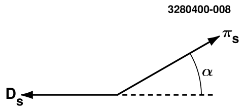
FIG. 3.: Definition of $\alpha$: the angle between the reverse direction of the measured $D_{s}^{+}$ and measured $\pi_{s}^{-}$.

It is possible to further constrain $\alpha$ from additional event information that determines the allowed $D^{*-}$ directions. There exist a total of eight unknowns in the decay: the $\bar{D}^{0}$ three-momentum, the parent $D^{*-}$ three-momentum, and the two angles governing the $B^{0}$ direction. The $B$ energy is equal to the CLEO beam energy. Requiring conservation of energy and momentum in the $B^{0}\rightarrow D_{s}^{+}D^{*-}$ and $D^{*-}\rightarrow\bar{D}^{0}\pi^{-}_{s}$ decays yields eight constraints, where the masses of the $B^{0}$, $D_{s}^{+}$, $D^{*-}$, $\bar{D}^{0}$, and $\pi^{-}$ are assumed. Solving for the unknowns yields a pair of $D^{*-}$ solutions, due to a quadratic ambiguity in the underlying algebra. The procedure of this solution follows.

The $D^{*-}$ and $\bar{D}^{0}$ energies are determined from the measured $D_{s}^{+}$ and $\pi_{s}^{+}$ energies:

$$E_{D^{*-}}=E_{Beam}-E_{D_{s}^{+}},$$ (8)

$$E_{\bar{D}^{0}}=E_{D^{*-}}-E_{\pi_{s}^{+}}.$$ (9)

The magnitude of $D^{*-}$ and $\bar{D}^{0}$ momenta follow from their energies $p_{D^{*-}}=\sqrt{E_{D^{*-}}^{2}-M_{D^{*-}}^{2}}$ and $p_{\bar{D}^{0}}=\sqrt{E_{\bar{D}^{0}}^{2}-M_{\bar{D}^{0}}^{2}}$. For the previously-assumed decay, kinematics constrain the $D^{*-}$ to a cone of allowed directions relative to the measured $D_{s}^{+}$. The radius of this cone, $\theta_{1}$, is shown in Figure 4, and represents the angle between the reverse $D_{s}^{+}$ direction and inferred $D^{*-}$. Using the $D_{s}^{+}$ momentum magnitude, beam energy, and particle masses, $\theta_{1}$ can be expressed in the lab frame as:

$$\cos{\theta_{1}}=\frac{M^{2}_{B^{0}}-M^{2}_{D^{*}}-M^{2}_{D_{s}}}{2|\vec{p}_{D_{s}}||\vec{p}_{D^{*}}|}-\frac{1}{\beta_{D_{s}}\beta_{D^{*}}}.$$ (10)

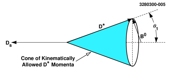
FIG. 4.: Definition of $\theta_{1}$: the angle between the reverse $D_{s}^{+}$ direction and the cone of allowed $D^{*-}$ directions.

Kinematics also constrain the $D^{*-}$ to a cone of allowed values about the $\pi_{s}^{-}$ direction. The radius of this cone is $\theta_{2}$, the angle between the $\pi_{s}^{-}$ and inferred $D^{*-}$, defined in the lab frame and shown in Figure 5:

$$\cos{\theta_{2}}=\frac{M^{2}_{D^{0}}-M^{2}_{D^{*}}-M^{2}_{\pi_{s}}}{2|\vec{p}_{\pi_{s}}||\vec{p}_{D^{*}}|}+\frac{1}{\beta_{\pi_{s}}\beta_{D^{*}}}.$$ (11)

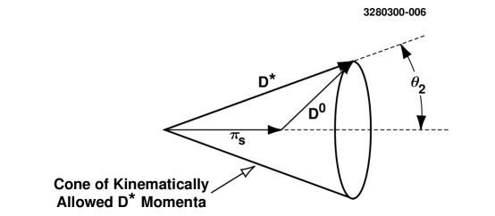
FIG. 5.: Definition of $\theta_{2}$: the angle between the $\pi_{s}^{-}$ and cone of allowed $D^{*-}$ directions.

Valid solutions for the $D^{*-}$ momentum exist at the intersection of the cones defined by $\theta_{1}$ and $\theta_{2}$, as shown in Figure 6. For the two cones to intersect, the angle between the measured $D_{s}^{+}$ and measured $\pi_{s}^{-}$—the angle previously defined as $\alpha$—must be confined to a range bounded by the sum and difference of $\theta_{1}$ and $\theta_{2}$:

$$|\theta_{1}-\theta_{2}|\leq\alpha\leq\theta_{1}+\theta_{2}.$$ (12)

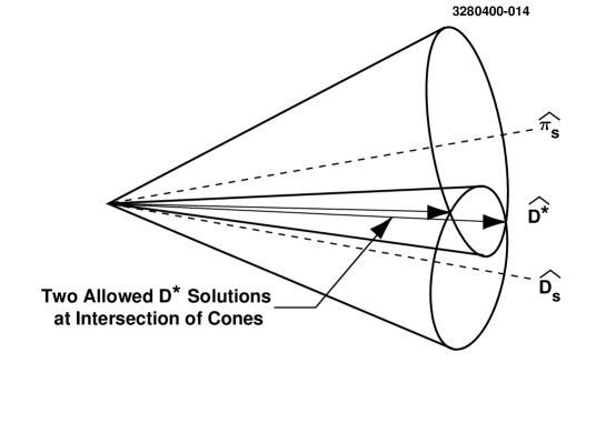
FIG. 6.: Valid $D^{*-}$ solutions exist where the combined $\theta_{1}$ and $\theta_{2}$ cones intersect. There are generally two solutions, resulting from a quadratic ambiguity in the underlying algebra.

For $\alpha$ greater than the upper limit $\theta_{1}+\theta_{2}$, the smaller cone is entirely outside the larger one, preventing their intersection and the existence of a kinematically valid $D^{*-}$ solution. For $\alpha$ less than the lower limit $|\theta_{1}-\theta_{2}|$, the smaller cone is completely inside the larger, also preventing their intersection. As shown in Figure 7, the lower limit occurs as the smaller cone grazes the inside edge of the larger one, where this limit is defined as $\alpha_{0}$:

$$\alpha_{0}\equiv|\theta_{1}-\theta_{2}|.$$ (13)

Since only one $\alpha$ and one $\alpha_{0}$ exist for a particular $(D_{s}^{+},\pi_{s}^{-})$ pair, they are unaffected by the quadratic ambiguity in the $D^{*-}$ solutions.

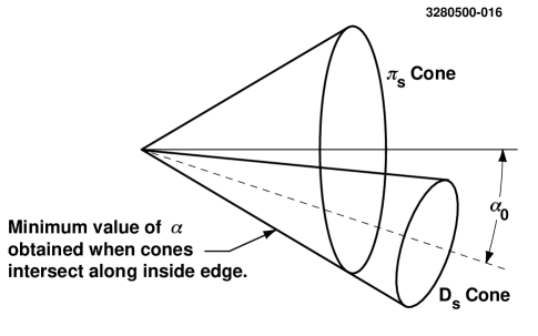
FIG. 7.: $\alpha_{0}$ is the minimum value $\alpha$ can take for an event where the cones continue to intersect, and corresponds to the smaller cone grazing the inside edge of the larger.

In the case of the signal $B^{0}\rightarrow D_{s}^{+}D^{*-}$ mode, $\alpha$ is small, $\alpha_{0}$ is as small or smaller, and the difference between $\alpha$ and $\alpha_{0}$ is very small. Since the background is relatively isotropic in $\cos{\alpha}$, it is more convenient to work with the cosines of the angles, where it is found that the difference $\cos{\alpha_{0}}-\cos{\alpha}$ peaks sharply for signal at small values. Signal Monte Carlo distributions are shown in Figure 8 over the range $(-0.04,2.00)$ for $D_{s}^{+}D^{*-}$, $D_{s}^{*+}D^{*-}$, and $D_{s}^{(*)+}D^{**}$. Two backgrounds are also shown in the figure: the $B\bar{B}$ background, from simulated non-signal $B$ meson events, and continuum background, from $e^{+}e^{-}\rightarrow c\bar{c}$, $s\bar{s}$, $u\bar{u}$, or $d\bar{d}$. The three signals display sharp peaking in $\cos{\alpha_{0}}-\cos{\alpha}$, where the $D_{s}^{*}D^{*}$ and $D_{s}^{(*)}D^{**}$ peaks are measurably broader than the $D_{s}D^{*}$. In the $D_{s}^{*+}D^{*-}$ case, this broadness results from the random nudge given the $D_{s}^{+}$ by the $\gamma/\pi^{0}$ in the $D_{s}^{*+}\rightarrow D_{s}^{+}\gamma/D_{s}^{+}\pi^{0}$ transition, causing the two particles to be not quite so back-to-back. For the $D_{s}^{(*)+}D^{**}$, the broad peak comes from the thrust given the $D^{*-}$ from the unreconstructed $\pi^{+}$ produced during the intermediate $\bar{D}^{**0}\rightarrow D^{*-}\pi^{+}$ decay. It should be noted that no sharp peaking occurs in either background where the $D_{s}^{+}$ and $\pi_{s}^{-}$ are nearly uncorrelated, though some hint of a peak is exhibited due to kinematic correlations.

It is seen from Figure 8 that $\cos{\alpha_{0}}-\cos{\alpha}$ occasionally drifts below zero. This is due to detector resolution effects that distort the quantities used to calculate $\cos{\theta_{1}}$ and $\cos{\theta_{2}}$.

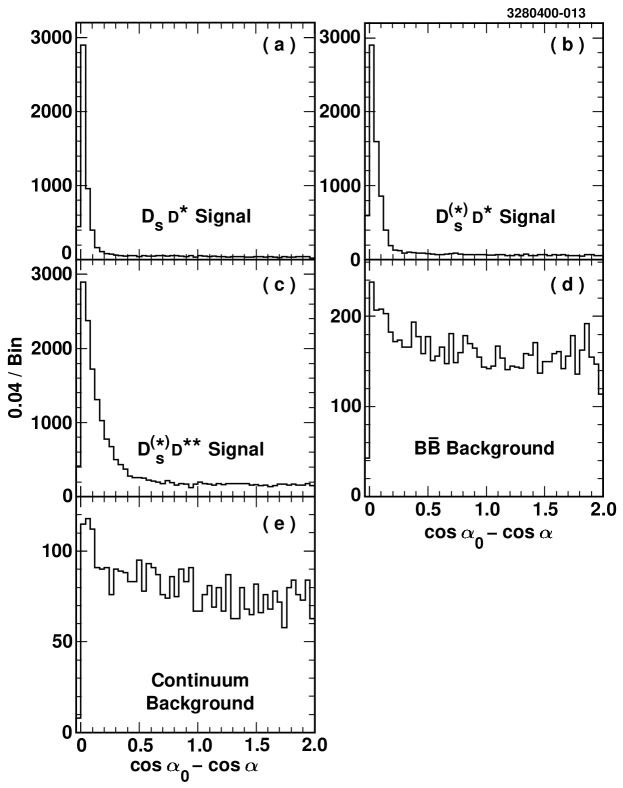
FIG. 8.: Signal Monte Carlo and background distributions of the partial-reconstruction variable $\cos{\alpha_{0}}-\cos{\alpha}$. Shown are: (a) $D_{s}D^{*}$ Monte Carlo, (b) $D_{s}^{*}D^{*}$ Monte Carlo, (c) $D_{s}^{(*)}D^{**}$ Monte Carlo, (d) $B\bar{B}$ background Monte Carlo, (e) continuum data. The signals display a characteristic narrow peak, while the backgrounds are relatively broad.

D Fit of the Data

A sharp signal peak in the $\cos{\alpha_{0}}-\cos{\alpha}$ distribution of the CLEO on-resonance data previously described in Section II, superimposed on a relatively flat background, is seen in Figure 9. The figure also shows a binned maximum-likelihood fit to this data consisting of three components: $D_{s}^{(*)}D^{*(*)}$ signal, $B\bar{B}$ background, and continuum background. The $D_{s}^{(*)}D^{*(*)}$ signal and $B\bar{B}$ background components are allowed to float, while the continuum level is fixed by scaling the off-resonance background by the on/off-resonance ratio. The $D_{s}^{(*)}D^{*(*)}$ component is a weighted combination of $D_{s}D^{*}$, $D_{s}^{*}D^{*}$, and $D_{s}^{(*)}D^{**}$ signals, as the signal distribution shapes in $\cos{\alpha_{0}}-\cos{\alpha}$ are too similar for meaningful separation. The signal is concentrated in the relatively small region $-0.04\leq\cos{\alpha_{0}}-\cos{\alpha}\leq 0.12$, where the data contains 528 events. Table III lists fit results of the three components for this signal region. The errors listed are statistical. The subsequent analysis of the relative $D_{s}^{(*)}D^{*(*)}$ rates and polarizations is confined to the signal region:

$$-0.04\leq\cos{\alpha_{0}}-\cos{\alpha}\leq 0.12$$ (14)

TABLE III.: Fit results for the data signal region $-0.04\leq\cos{\alpha_{0}}-\cos{\alpha}\leq 0.12$, containing 528 events. Errors are statistical.

Mode	Number of events
$D_{s}^{(*)}D^{*(*)}$ Signal	$314.0\pm 24.0$
$B\bar{B}$ Background	$138.9\pm 5.2$
Continuum	$74.8$ (constrained)

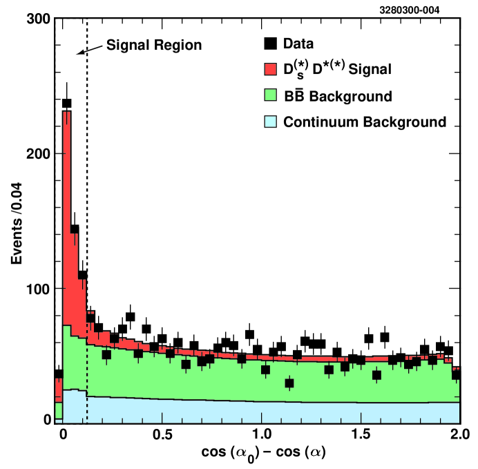
FIG. 9.: The fitted $\cos{\alpha_{0}}-\cos{\alpha}$ data distribution. The fit is broken down into three components: $D_{s}^{(*)}D^{*(*)}$ signal, $B\bar{B}$ background, and continuum background. The signal region is $-0.04\leq\cos{\alpha_{0}}-\cos{\alpha}\leq 0.12$. The continuum background is constrained by scaling the off-resonance background by the on/off-resonance ratio.

V SEPARATION OF $D_{s}D^{*}$, $D_{s}^{*}D^{*}$, AND $D_{s}^{(*)}D^{**}$ SIGNALS. MEASUREMENT OF $D_{s}^{*}D^{*}$ POLARIZATION

A Definition of the Two-Dimensional $p_{D_{s}}$ vs $\cos{\theta_{\pi}}$ Parameter Space

Once the background levels have been determined, the signal modes may be separated from one another. This separation is effected by constructing a two-dimensional parameter space, where each signal carries a distinctive shape. Two variables are required, of which the first is the magnitude of $D_{s}^{+}$ momentum $p_{D_{s}}$. The kinematics of the $B\rightarrow D_{s}^{(*)}D^{*(*)}$ decays constrain the relevant $D_{s}$ momentum range to $1250\ {\rm MeV}/c\leq p_{D_{s}}\leq 1925\ {\rm MeV}/c$. The second variable of interest is the cosine of the $\pi_{s}^{-}$ decay angle as expressed in the $D^{*-}$ frame—$\cos{\theta_{\pi}}$—where $\theta_{\pi}$ is a helicity angle, shown in Figure 10. It is possible to calculate $\cos{\theta_{\pi}}$ from available event information, without reconstructing the $D^{*-}$:

$$\cos{\theta_{\pi}}=-\frac{\beta_{D^{*}}(E^{*}_{\pi_{s}}-E^{*}_{D^{0}})}{2p^{*}_{D^{0}}}+\frac{p^{2}_{\pi_{s}}-p^{2}_{D^{0}}}{2\gamma^{2}_{D^{*}}\beta_{D^{*}}M_{D^{*}}p^{*}_{D^{0}}}$$ (15)

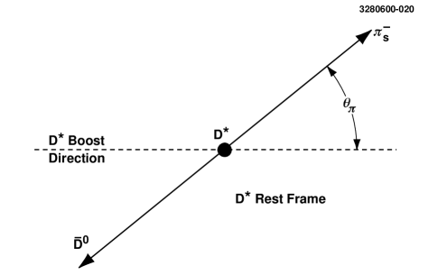
FIG. 10.: Defining $\cos{\theta_{\pi}}$: the decay angle of the $\pi_{s}$ as measured in the $D^{*}$ rest frame.

Here the kinematics of the $B^{0}\rightarrow D_{s}^{+}D^{*-}$ mode have been assumed. The quantities $\gamma_{D^{*}}$, $\beta_{D^{*}}$, $p_{\pi_{s}}$, and $p_{D_{s}}$ are expressed in the lab frame, while $E^{*}_{\pi_{s}}$, $E^{*}_{D^{0}}$, and $p^{*}_{D^{0}}$ are in the $D^{*-}$ frame,

$$E^{*}_{D^{0}}=\frac{M^{2}_{D^{*}}+M^{2}_{D^{0}}-M^{2}_{\pi_{s}}}{2M_{D^{*}}}$$ (16)

$$E^{*}_{\pi_{s}}=\frac{M^{2}_{D^{*}}-M^{2}_{D^{0}}+M^{2}_{\pi_{s}}}{2M_{D^{*}}}.$$ (17)

In the $B^{0}\rightarrow D_{s}^{+}D^{*-}$ mode, the $D^{*-}$ is produced in a $(J,J_{z})=(1,0)$ state, and conservation of helicity distributes the $\pi_{s}^{-}$ as $\cos^{2}{\theta_{\pi}}$. Imperfect detector resolution smears the shape. For the case of longitudinally polarized $D_{s}^{*+}D^{*-}$ from $B^{0}$ decays, the $D^{*-}$ is also produced in a $(1,0)$ state. However, the resulting $\cos^{2}{\theta_{\pi}}$ shape is not centered at the origin, but is rather shifted downwards. This shift comes from the missing $\gamma/\pi^{0}$ (where $D_{s}^{*+}\rightarrow D_{s}^{+}\gamma/D_{s}^{+}\pi^{0}$), which was not taken into account in the calculation of $\cos{\theta_{\pi}}$. Nevertheless the original $\cos^{2}{\theta_{\pi}}$ shape is well preserved, centered at $-0.2$, and falls over the range $(-1.2,0.8)$. In the case of transversely polarized $D_{s}^{*+}D^{*-}$, the $D^{*-}$ is produced in a $(1,1)$ or $(1,-1)$ state, and the resulting $\pi_{s}^{-}$ produces a helicity distribution of $1-\cos^{2}{\theta_{\pi}}$, also centered at $-0.2$. Finally, the three $D^{**0}$ states each produce the $\pi_{s}^{-}$ in their unique helicity distributions: the $D_{1}(2420)^{0}$ decays as $1+3\cos^{2}{\theta_{\pi}}$, the $D_{2}^{*}(2460)^{0}$ decays as $1-\cos^{2}{\theta_{\pi}}$, and the $D_{1}(j=1/2)^{0}$ decays isotropically. However, blending the three $D^{**0}$ states according to their production ratios in $D_{s}^{+}D^{**}$ and $D_{s}^{*+}D^{**}$ effectively washes out any characteristic helicity shape. The resulting blended distribution is centered at $-0.4$ and ranges over $(-1.4,0.5)$, because of the missing intermediate $\pi$ (from $D^{**}\rightarrow D^{*-}\pi$), which is not accounted for in calculating $\cos{\theta_{\pi}}$. The limits of $\cos{\theta_{\pi}}$ relevant to this analysis are therefore $-1.40\leq\cos{\theta_{\pi}}\leq 1.05$.

The $p_{D_{s}}$ versus $\cos{\theta_{\pi}}$ two-dimensional distributions are shown in Figure 11 for each of the four signals ($D_{s}D^{*}$, Longitudinally Polarized $D_{s}^{*}D^{*}$, Transversely Polarized $D_{s}^{*}D^{*}$, and $D_{s}^{(*)}D^{**}$) and two backgrounds ($B\bar{B}$ and continuum). Because the longitudinally polarized and transversely polarized $D_{s}^{*}D^{*}$ produce markedly different shapes in this two-dimensional distribution, they can be separated into two components. The two-dimensional on-resonance CLEO data distribution is shown in Figure 12.

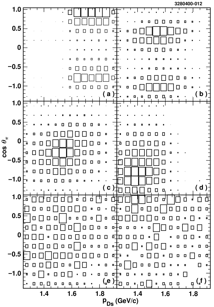
FIG. 11.: $p_{D_{s}}$ vs $\cos{\theta_{\pi}}$ distributions for the four signal Monte Carlo and two background samples. Shown are: (a) $D_{s}D^{*}$ Monte Carlo, (b) Longitudinally Polarized $D_{s}^{*}D^{*}$ Monte Carlo, (c) Transversely Polarized $D_{s}^{*}D^{*}$ Monte Carlo, (d) $D_{s}^{(*)}D^{**}$ Monte Carlo, (e) $B\bar{B}$ background Monte Carlo, (f) continuum data. The box size is proportional to the number of candidates in the bin.

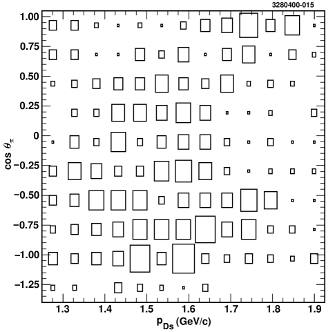
FIG. 12.: $p_{D_{s}}$ vs $\cos{\theta_{\pi}}$ distributions for the CLEO data. The plot contains 528 events. The box size is proportional to the number of candidates in the bin.

B The Fitted Data

A two-dimensional binned maximum-likelihood fit is applied to the data. The $B\bar{B}$ and continuum backgrounds, whose levels were determined in the previous one-dimensional fit to the $\cos{\alpha_{0}}-\cos{\alpha}$ distribution, are fixed here, and their shapes are parameterized as products of Chebyshev polynomials. The two-dimensional Monte Carlo distributions are used for the $D_{s}^{(*)}D^{*(*)}$ signals. Four signal components are allowed to float: the number of $D_{s}D^{*}$, number of $D_{s}^{*}D^{*}$, number of $D_{s}^{(*)}D^{**}$, and the relative longitudinal $D_{s}^{*}D^{*}$ polarization. Converting the likelihood to a $\chi^{2}$-like quantity ($-2\ln{\mathcal{L}}$), the resulting fit has a likelihood of 125.4 for 130 bins with 4 floating parameters. Projections of data and fit along both the $p_{D_{s}}$ and $\cos{\theta_{\pi}}$ axes, broken down into signal and background components, are shown in Figure 13. In Table IV, the number of events resulting from the two-dimensional maximum-likelihood fit are reported for each of the $D_{s}^{(*)+}D^{*(*)}$ modes, along with their statistical and systematic uncertainties, where the systematics will be discussed in Section VI.

TABLE IV.: Fitted yield for each $D_{s}^{(*)+}D^{*(*)}$ mode. The first error is statistical and the second is systematic. The $D^{**}$ is the sum of charged and neutral $D_{1}(2420)$, $D^{*}_{2}(2460)$, and $D_{1}(j=1/2)$ resonances.

Mode	Fitted Yield
$B^{0}\rightarrow D_{s}^{+}D^{*-}$	$92.7\pm 15.3\pm 9.5$
$B^{0}\rightarrow D_{s}^{*+}D^{*-}$	$149.2\pm 30.4\pm 20.9$
$B\rightarrow D_{s}^{(*)+}D^{**}$	$81.6\pm 23.3\pm 15.3$

The relative longitudinal polarization of the $D_{s}^{*+}D^{*-}$ production is measured to be:

$$\Gamma_{L}/\Gamma=(50.6\pm 13.9\pm 3.6)\%$$ (18)

where the first error is statistical and the second systematic.

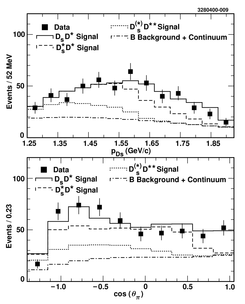
FIG. 13.: The projections of the two-dimensional CLEO data and fit along the $p_{D_{s}^{+}}$ axis (top) and $\cos{\theta_{\pi}}$ axis (bottom). The fit contains $D_{s}D^{*}$, $D_{s}^{*}D^{*}$, $D_{s}^{(*)}D^{**}$, and background components.

C The Fitted Data With the $D_{s}^{(*)+}D^{**}$ Component Removed

Because production of $B\rightarrow D_{s}^{(*)+}D^{**}$ has not been previously observed, one might question its inclusion in the preceding fit. A worthwhile consistency check is to remove the $D_{s}^{(*)+}D^{**}$ from the set of functions and repeat the two-dimensional fitting procedure. The results, without the $D_{s}^{(*)+}D^{**}$, are projected along the $p_{D_{s}}$ axis and $\cos{\theta_{\pi}}$ axis in Figure 14. The $p_{D_{s}}$ fit projection shape matches the data well, but is shifted systematically upwards by about 50 MeV/$c$. The $\cos{\theta_{\pi}}$ fit projection shape is decidedly different from the data, since the projection is systematically low over the region $-1.2\leq\cos{\theta_{\pi}}\leq-0.2$ and systematically high over the region $-0.2\leq\cos{\theta_{\pi}}\leq 0.8$. The $\cos{\theta_{\pi}}$ fit projection also displays a pair of symmetric peaks that are not reflected in the data. This two-dimensional fit has a likelihood of 139.9 for 130 bins with three floating parameters, and since for this fitting procedure the likelihood follows closely the $chi^{2}$ behavior, this corresponds to a reduced significance of 3.8 standard deviations. A study of the data sideband regions off the $\cos{\alpha_{0}}-\cos{\alpha}$ signal peak (i.e. where $\cos{\alpha_{0}}-\cos{\alpha}\geq 0.12$) reveals an amount of $D_{s}^{(*)+}D^{**}$ that is consistent with the amount of $D_{s}^{(*)+}D^{**}$ observed in the signal region $-0.04\leq\cos{\alpha_{0}}-\cos{\alpha}\leq 0.12$. Taking the factors all together, we conclude that the data strongly indicate a substantial $D_{s}^{(*)+}D^{*(*)}$ component.

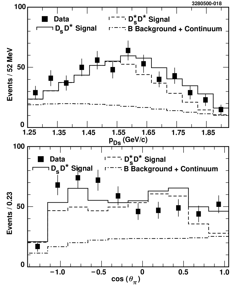
FIG. 14.: Removing the $D_{s}^{(*)}D^{**}$ component from the two-dimensional fit to the CLEO data, where data and fit are projected along the $p_{D_{s}^{+}}$ axis (top) and $\cos{\theta_{\pi}}$ axis (bottom). The fit is split into $D_{s}D^{*}$, $D_{s}^{*}D^{*}$, and background components. The $p_{D_{s}}$ fit projection shape is shifted upwards relative to the data, and the ${\theta_{\pi}}$ fit projection shape is systematically low over the region $-1.2\leq\cos{\theta_{\pi}}\leq-0.2$ and systematically high over the region $-0.2\leq\cos{\theta_{\pi}}\leq 0.8$. The likelihood is reduced by 3.8 standard deviations from the previous fit, which includes a $D_{s}^{(*)}D^{**}$ component.

VI SYSTEMATIC UNCERTAINTIES

The single largest uncertainty in the analysis is the 25% uncertainty in the $D_{s}^{+}\rightarrow\phi\pi^{+}$ branching fraction[8]:

$${\mathcal{B}}(D_{s}^{+}\rightarrow\phi\pi^{+})=(3.6\pm 0.9)\%$$ (19)

This uncertainty is displayed separately from the other systematic uncertainties, which are listed in Table V.

TABLE V.: Systematic uncertainties in percent for $B\rightarrow D_{s}^{(*)+}D^{*(*)}$ decays and $\Gamma_{L}/\Gamma$, the longitudinal polarization of $D_{s}^{*+}D^{*-}$ .

Source	$D_{s}^{+}D^{*-}$	$D_{s}^{*+}D^{*-}$	$D_{s}^{(*)+}$	$\Gamma_{L}/\Gamma$
			$D^{**}$
$D_{s}$ Tracking	3.0	3.0	3.0	3.0
$\pi_{s}$ Tracking	5.0	5.0	5.0	5.0
Total Number of	1.8	1.8	1.8	—
$B\bar{B}$ Mesons
Fit Normalization	2.9	2.9	2.9	—
Monte Carlo Statistics	1.0	1.0	1.0	1.0
Continuum Subtraction	3.7	3.7	3.7	1.8
$B\bar{B}$ Background	1.6	1.6	1.6	1.0
Subtraction
Continuum Shape	1.0	1.0	1.0	1.0
$B\bar{B}$ Background	1.0	1.0	1.0	1.0
Shape
$D_{1}(j=1/2):D_{1}(2420):$	0.8	2.9	4.5	0.6
$D_{2}^{*}(2460)$ ratio
$D_{s}^{+}D^{**}:D_{s}^{*+}D^{**}$ Ratio	2.4	9.8	14.8	3.2
Non-Resonant	2.2	4.5	5.9	1.2
$D_{s}^{(*)+}D^{*-}\pi$ Production
Total for $D_{s}^{(*)+}D^{*(*)}$ yield	9.9	13.8	18.5	—
${\mathcal{B}}(\phi\rightarrow K^{+}\,K^{-})$	1.6	1.6	1.6	—
${\mathcal{B}}(D^{*-}\rightarrow\bar{D}^{0}\,\pi_{s}^{-})$	2.0	2.0	2.0	—
Total systematic uncertainty	10.2	14.0	18.7	7.3

A 1% systematic uncertainty in track finding and fitting efficiency is estimated for each fast charged track, which for the $D_{s}^{+}$ add linearly to a 3% total. The slow pion $\pi_{s}$ track finding and fitting uncertainty is estimated at 5%. The uncertainty in the total number of $B\bar{B}$ meson pairs introduces a systematic error of 1.8%.

The two-dimensional fit to the data estimates the total amount of $D_{s}^{(*)}D^{*(*)}$ signal at 323.2 events. Since the previous one-dimensional fit to the $\cos{\alpha_{0}}-\cos{\alpha}$ distribution, summarized in Table III, determined the level of $D_{s}^{(*)}D^{*(*)}$ signal at $314.0\pm 24.0$, the two-dimensional fit result overestimates the amount of signal by 9.2 events. To test for a systematic bias in the two-dimensional fitting procedure, fifty simulated datasets were created and filled with $D_{s}^{(*)}D^{*(*)}$ signal Monte Carlo, $B\bar{B}$ background, and continuum background according to the proportions of Tables III and IV. Following the procedure of fixing both backgrounds and allowing all four signal components to float, two-dimensional fits to these simulated datasets gave fifty estimates of total $D_{s}^{(*)}D^{*(*)}$ signal. The difference between the estimate from each fit and the number of input $D_{s}^{(*)}D^{*(*)}$ events forms a distribution centered at 1.1 with an rms of 5.3, consistent with zero and indicative of an unbiased fitting procedure. In the case of the fit to the real dataset, the additional 9.2 events differ from the expected total by an acceptable 1.7 standard deviations. In order that these events might be accounted for, a systematic error of 2.9% is introduced into the overall signal yield. The polarization measurement is not affected by this systematic error in the fit normalization.

Forty thousand signal Monte Carlo events were generated for each of the nine signal modes: $D_{s}^{+}D^{*-}$, longitudinally polarized $D_{s}^{*+}D^{*-}$, transversely polarized $D_{s}^{*+}D^{*-}$, $D_{s}^{+}\bar{D}^{**0}$ (for each of $\bar{D}_{1}(2420)^{0}$, $\bar{D}_{2}^{*}(2460)^{0}$, and $\bar{D}_{1}(j=1/2)^{0}$) and $D_{s}^{*+}\bar{D}^{**0}$ (also for all three $\bar{D}^{**0}$ states). To estimate statistical limitations, the signal samples were divided in half and the half-samples used to refit the two-dimensional $p_{D_{s}^{+}}$ vs $\cos{\theta_{\pi}}$ data distribution. The resulting fits differ from the original by less than 1.0%.

An uncertainty is introduced by statistical fluctuations in the amount of continuum background. Varying the number of continuum background events by one standard deviation ($\sigma$) affects the overall two-dimensional fit yields by a maximum of 3.7% and the polarization by a maximum of 1.8%. The uncertainty from statistical fluctuations in the total number of $B\bar{B}$ background events is anti-correlated with the continuum background. This is the result of highly similar background shapes in the one-dimensional fit to the $\cos{\alpha_{0}}-\cos{\alpha}$ data distribution. Refitting the two-dimensional data distribution with these fluctuations changes the yields by a maximum of 1.6%, and the polarization by a maximum of 1.0%, where the small uncertainty results from the anticorrelation.

The two-dimensional continuum and background shapes are parameterized as products of Chebyshev polynomials. Varying the polynomial coefficients by the parameterization errors and refitting the two-dimensional data distribution changes the results by less than 1.0% for either background.

In the two-dimensional fit to the data distribution, there is a single component containing $D_{s}^{(*)+}D^{**}$ signal. The $D^{**}$ label denotes the sum of three $L=1$ charm states: the $D_{1}(j=1/2)$, $D_{1}(2420)$, and the $D_{2}^{*}(2460)$. Each of these three states has a unique mass and width, and produces a different pattern of $\pi_{s}^{-}$ helicities. In building the $D^{**}$ signal component, it is assumed that the $D^{**}$ production rate from $B$ mesons is at a $D_{1}(j=1/2):D_{1}(2420):D_{2}^{*}(2460)$ ratio of $2:1:6.7$, in accordance with the known $D_{1}(2420)$ and $D_{2}^{*}(2460)$ production rates in $B\rightarrow D^{**}\pi$[13] and the preliminary evidence for the $D_{1}(j=1/2)$[15]. To understand the systematic bias introduced by this choice of ratios, the data was refit using widely varying ratios of ($2:1:3.3$, $2:1:13.5$, $1:1:6.7$, $4:1:6.7$, $2:2:6.7$, and $2:0.5:6.7$). This caused the $D_{s}D^{*}$ yield to vary by 0.8%, the $D^{*}_{s}D^{*}$ yield to vary by as much as 2.9%, the $D_{s}^{(*)}D^{**}$ yield to vary by 4.5%, and the polarization to vary by 0.6%.

The $D_{s}^{+}D^{**}:D^{*+}_{s}D^{**}$ ratio in the $D_{s}^{(*)}D^{**}$ component has been fixed a priori at $1:2$ in the two-dimensional fit. The assumption of this ratio follows from the analogous modes $B\rightarrow D_{s}^{(*)}D^{*}$, where $D_{s}D^{*}:D^{*}_{s}D^{*}$ has been previously measured at $1:2$, a ratio confirmed by this analysis. The pseudoscalar/vector $D_{s}:D^{*}_{s}$ ratio in this spectator decay implies that the same ratio should hold for the $D_{s}^{(*)}D^{**}$ case as well. All the decays $B^{0}\rightarrow D_{s}^{(*)+}\bar{D}^{*(*)}$ are spectator decays described by a single Feynman diagram and differentiated only by the final angular momentum states of the $c\bar{s}$ ($D_{s}^{+}$ or $D_{s}^{*+}$) and $\bar{c}q$ ($D^{*}$ or $D^{**}$) quark pairs. To be particularly conservative, the $D_{s}D^{**}:D^{*}_{s}D^{**}$ ratio is allowed to vary between $1:1$ and $1:4$. Pseudoscalar/vector spin considerations strongly suggest that the ratio be confined between these two limits. Varying the $D_{s}^{+}D^{**}:D^{*+}_{s}D^{**}$ ratio between $1:1$ and $1:4$ changes the fit results significantly, as the $D_{s}^{+}D^{*-}$ varies by a maximum of 2.4%, the $D_{s}^{*+}D^{*-}$ by 9.8%, the $D^{(*)+}D^{**}$ by 14.8%, and the polarization by 3.2%. These errors are the second largest systematic uncertainty, after the $D_{s}^{+}\rightarrow\phi\pi^{+}$ branching fraction uncertainty.

There exists the possibility that significant non-resonant $B\rightarrow D_{s}^{(*)+}D^{*}\pi$ production could contribute to the data sample. The three-body $B\rightarrow D_{s}^{(*)+}D^{*}\pi$ decay peaks nearly as strongly as resonant signal in $\cos{\alpha_{0}}-\cos{\alpha}$. While no measurements of the $B\rightarrow D_{s}^{(*)+}D^{*-}\pi$ non-resonant production have been made, an analogy can be drawn to non-resonant production of $B\rightarrow D^{*-}\pi\ell\nu$. ALEPH has measured the inclusive branching fraction $B\rightarrow D^{*-}\pi\ell^{-}\nu$ at $(1.25\pm 0.25)\%$, and the product of exclusive branching fractions ${\mathcal{B}}(\bar{B}\rightarrow D_{1}(2420)\ell^{-}\nu){\mathcal{B}}(D_{1}(2420)^{0}\rightarrow D^{*}\pi)=(0.52\pm 0.17)\%$[16]. ALEPH has also placed an upper limit on the $D_{2}^{*}(2460)$ branching fraction at ${\mathcal{B}}(\bar{B}\rightarrow D_{2}^{*}(2460)\ell^{-}\nu){\mathcal{B}}(D_{2}^{*}(2460)\rightarrow D^{*}\pi)<0.39\%$[16]. Although there is no measurement of the mode $\bar{B}\rightarrow D_{1}(j=1/2)\ell^{-}\nu$, recent observations at CLEO of the related mode $B^{+}\rightarrow\bar{D}^{**0}\pi^{+}$ report ${\mathcal{B}}(B\rightarrow\bar{D}_{1}(2420)^{0}\pi^{+})\approx 2/3{\mathcal{B}}(B^{+}\rightarrow\bar{D}_{1}(j=1/2)^{0}\pi^{+})\approx 2/3{\mathcal{B}}(B^{+}\rightarrow\bar{D}_{2}^{*}(2460)^{0}\pi^{+})$[15]. Assuming that ${\mathcal{B}}(\bar{D}_{1}(2420)^{0}\rightarrow D^{*-}\pi^{+})={\mathcal{B}}(\bar{D}_{1}(j=1/2)^{0}\rightarrow D^{*-}\pi^{+})=2/3$ and ${\mathcal{B}}(\bar{D}_{2}^{*}(2460)^{0}\rightarrow D^{*-}\pi^{+})=1/5$, and assuming that these relative $D^{**}\pi$ ratios hold in the semileptonic case, nearly all of the inclusive $B\rightarrow D^{*-}\pi\ell^{-}\nu$ will be accounted for by resonant $B\rightarrow D^{**}\ell^{-}\nu$. This would leave only a small nonresonant component. Thus a conservative upper limit is that non-resonant $B\rightarrow D_{s}^{(*)+}D^{*-}\pi$ could be as large as 40% of the resonant $B\rightarrow D_{s}^{(*)+}D^{**}$ branching fraction. Three $B\rightarrow D_{s}^{(*)}D^{**}$ $+$ (Non-Resonant) samples were created: one that contained 60% pure $B\rightarrow D^{(*)+}D^{**}$ with 30% non-resonant $B\rightarrow D_{s}^{+}D^{*-}\pi$ and 10% $B\rightarrow D^{*+}_{s}D^{*-}\pi$, one that contained 60% pure $B\rightarrow D_{s}^{(*)+}D^{**}$ with 10% non-resonant $B\rightarrow D_{s}^{+}D^{*-}\pi$ and 30% non-resonant $B\rightarrow D^{*+}_{s}D^{*-}\pi$, and one that contained 60% pure $B\rightarrow D_{s}^{(*)+}D^{**}$ with 20% non-resonant $B\rightarrow D_{s}^{+}D^{*-}\pi$ and 20% non-resonant $B\rightarrow D^{*+}_{s}D^{*-}\pi$. Refitting the data distribution with these $B\rightarrow D_{s}^{(*)+}D^{**}$ $+$ non-resonant $B\rightarrow D_{s}^{(*)+}D^{*-}\pi$ samples changes the results by 2.2% for the $B\rightarrow D_{s}^{+}D^{*-}$ case, by 4.5% for the $B\rightarrow D^{*+}_{s}D^{*-}$, by 5.9% for the $B\rightarrow D_{s}^{(*)+}D^{**}$, and by 1.2% for the polarization. These are the systematic errors listed in Table V. Should it be the case that by 60% of resonant $B\rightarrow D_{s}^{(*)+}D^{**}$ branching fraction be non-resonant, the systematic errors increase would increase to 3.0% for the $B\rightarrow D_{s}^{+}D^{*-}$, to 6.3% for the $B\rightarrow D^{*+}_{s}D^{*-}$, to 8.1% for the $B\rightarrow D_{s}^{(*)+}D^{**}$, and to 1.8% for the polarization. It should be noted that other non-resonant modes, such as $B\rightarrow D_{s}^{+}D^{*-}\pi\pi$, produce the $D_{s}^{+}$ in a momentum range that is almost entirely below the lower limit of 1250 MeV/$c$, excluding these modes from this analysis.

The 1998 PDG values for the $\phi$ and $D^{*-}$ branching fractions are ${\mathcal{B}}(\phi\rightarrow K^{+}K^{-})=(49.1\pm 0.8)\%$ and ${\mathcal{B}}(D^{*-}\rightarrow\bar{D}^{0}\pi_{s}^{-})=(68.3\pm 1.4)\%$[12]. These introduce systematic errors of 1.6% and 2.0%, respectively, into the extraction of the $D_{s}^{(*)+}D^{*(*)}$ branching fractions.

It is assumed in measuring the longitudinal and transverse $D_{s}^{*+}D^{*-}$ polarizations that these final states are independent of one another. In actuality there exists, in the differential decay rate, an interference term between the longitudinal and transverse states that is proportional to the azimuthal angle between the planes of the $D_{s}^{*+}\rightarrow D_{s}^{+}\gamma$ and $D^{*-}\rightarrow\bar{D}^{0}\pi^{-}$ decays. This interference vanishes in the integral over the azimuth, and introduces no systematic error into the analysis.

VII FACTORIZATION AND PREDICTION OF POLARIZATIONS

The factorization assumption, when expressed in the framework of Heavy Quark Effective Theory (HQET) and extrapolating from the form factors measured by the semileptonic $B$ decays $B\rightarrow D^{*}\ell\nu$, allows accurate estimate of the hadronic decay rates for the modes $B\rightarrow D^{(*)}\pi$, $D^{(*)}\rho$, $D_{s}^{(*)}D^{(*)}$, and $D^{(*)}D^{(*)}$[2, 18, 19, 20]. Additionally, factorization, HQET, and the semileptonic decays, predict the relative polarization of the vector-vector hadron products for $B\rightarrow D^{*-}X$ decays, such as $B\rightarrow D^{*-}\rho$ and $B^{0}\rightarrow D_{s}^{*+}D^{*-}$[21, 22].

We observe a longitudinal polarization in $B^{0}\rightarrow D_{s}^{*+}D^{*-}$ of $\Gamma_{L}/\Gamma=(50.6\pm 13.9\pm 3.6)\%$ for $q^{2}=M^{2}_{D_{s}^{*}}$, where the first error is statistical and the second systematic. The observation is consistent with the prediction of $(53.5\pm 3.3)\%$ from factorization, HQET, and the semileptonic form factor measurements[21]. The same combination also predicts in $B\rightarrow D^{*-}\rho$ a longitudinal polarization of $\Gamma_{L}/\Gamma=(89.5\pm 1.9)\%$ at $q^{2}=M_{\rho}^{2}$, which compares favorably with the most recent measurement of $(87.8\pm 5.3)\%$[23]. Finally, predictions are also made that at low $q^{2}$ the longitudinal polarization will be nearly 100%, and at $q^{2}=q^{2}_{max}$ decreases to 33%[2]. Longitudinal polarization as a function of $q^{2}$ is plotted in Figure 15 for the factorization prediction and compared with the $D^{*-}\rho$ and $D_{s}^{*+}D^{*-}$ measurements. The agreement is excellent, confirming the validity of the factorization assumption and HQET in extrapolating the semileptonic form factor results for regions of high $q^{2}$. The polarization of the semileptonic decays remains unobserved[22].

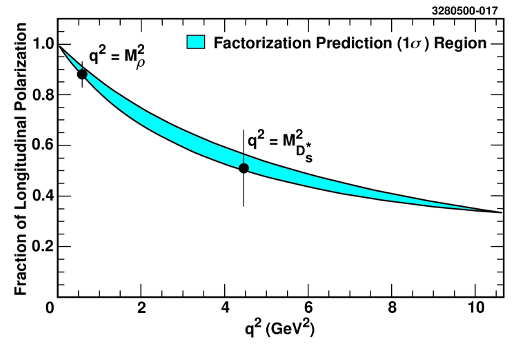
FIG. 15.: Relative fraction of longitudinal polarization in vector-vector $B\rightarrow D^{*-}X$ decays as a function of $q^{2}$, where $q^{2}=M^{2}_{X}$, and $X$ is a vector meson. Shown are the 1998 measurement of $B\rightarrow D^{*-}\rho$, and the $B^{0}\rightarrow D_{s}^{*+}D^{*-}$ polarization measured here for the first time. The shaded region represents the prediction using factorization and Heavy Quark Effective Theory, and extrapolating from the semileptonic $B\rightarrow D^{*}\ell\nu$ form factor results. The contour is one standard deviation ($\sigma$).

Another vector-vector hadronic $B$ decay mode which may further test the factorization assumption at high $q^{2}$ is $B^{0}\rightarrow D^{*+}D^{*-}$. This decay is Cabibbo-suppressed, and a polarization measurement will require higher statistics than those provided by present experiments[24]. Future experiments will also reduce the errors of the $D^{*-}\rho$ and $D_{s}^{*+}D^{*-}$ measurements.

VIII SUMMARY AND CONCLUSIONS

Removing the $D_{s}^{(*)+}D^{**}$ signal component from the two-dimensional fit reduces the likelihood by $3.8\sigma$, and the resulting projections along both the $p_{D_{s}}$ and $\cos{\theta_{\pi}}$ axes are systematically different from the data as discussed in Section V C. Furthermore, a level of $D_{s}^{(*)+}D^{**}$ is observed in the data sideband regions of $\cos{\alpha_{0}}-\cos{\alpha}$ consistent with that seen in the signal region. We conclude that the data support first evidence for $B\rightarrow D_{s}^{(*)+}D^{**}$ decays.

From the event yield of Table IV, we can calculate the exclusive branching fractions $B^{0}\rightarrow D_{s}^{+}D^{*-}$, $B^{0}\rightarrow D_{s}^{*+}D^{*-}$, and $B^{+}\rightarrow D_{s}^{(*)+}\bar{D}^{**0}$, where the $\bar{D}^{**0}$ is the sum of the $D_{1}(2420)^{0}$, $D^{*}_{2}(2460)^{0}$, and $D_{1}(j=1/2)^{0}$ states

$${\mathcal{B}}(B^{0}\rightarrow D_{s}^{+}\,D^{*-})=(1.10\pm 0.18\pm 0.11\pm 0.28)\%,$$ (20)

$${\mathcal{B}}(B^{0}\rightarrow D_{s}^{*+}\,D^{*-})=(1.82\pm 0.37\pm 0.25\pm 0.46)\%,$$ (21)

$${\mathcal{B}}(B^{+}\rightarrow D_{s}^{(*)+}\,\bar{D}^{**0})=(2.73\pm 0.78\pm 0.51\pm 0.68)\%.$$ (22)

The first error is statistical, the second systematic, and the third the contribution from the uncertainty of the $D_{s}^{+}\rightarrow\phi\pi^{+}$ branching fraction. These $B^{0}\rightarrow D_{s}^{(*)+}D^{*-}$ branching fractions supersede the previous CLEO measurements[1]. The extraction of the combined $D_{s}^{(*)+}\bar{D}^{**0}$ branching fraction is contingent on the assumption of Equation (7), where the charged-$B$ decay rate, $B^{+}\rightarrow D_{s}^{(*)+}\bar{D}^{**0}$, is presumed equal to the neutral-$B$ decay rate, $B^{0}\rightarrow D_{s}^{(*)+}D^{**-}$. The extraction also requires some presumption of the individual $D^{**}\rightarrow D^{*-}\pi$ rates, shown in Equations (1)–(6). The assumptions follow from conservation of isospin in the spectator $B$ decay of Figure 1. It is further assumed that the production rates of $B^{+}$ and $B^{0}$ in $\Upsilon(4S)$ decays are equal for all branching fraction measurements.

The relative longitudinal $D_{s}^{*}$ polarization in $B^{0}\rightarrow D_{s}^{*+}D^{*-}$ is measured for the first time as:

$$\frac{\Gamma_{L}}{\Gamma}(B^{0}\rightarrow D_{s}^{*+}D^{*-})=(50.6\pm 13.9\pm 3.6)\%$$ (23)

where the first error is statistical and the second systematic. The measurement is consistent with the recent factorization prediction of $(53.5\pm 3.3)\%$, confirming the validity of the factorization assumption in the domain of relatively high $q^{2}$[21].

REFERENCES

[1]
CLEO Collaboration, D. Gibaut et al., Phys. Rev. D 53, 4734 (1996).
[2]
J.L. Rosner, Phys. Rev. D 41, 3732 (1990).
[3]
A. Falk and M. Luke, Phys. Lett. B 292, 119 (1992).
[4]
M. Neubert, Phys. Lett. B 264, 455 (1991).
[5]
V. Rieckert, Phys. Rev. D 47, 3053 (1993).
[6]
G. Kramer, T. Mannel, and W.F. Palmer, Z. Phys. C 55, 497 (1992).
[7]
ARGUS Collaboration, H. Albrecht et al., Z. Phys. C 48, 543
(1990).
[8]
CLEO Collaboration, M. Artuso et al., Phys. Lett. B 378, 364
(1996).
[9]
CLEO Collaboration, G. Brandenberg et al., Phys. Rev. Lett. 80,
2762 (1998).
[10]
CLEO Collaboration, Y. Kubota et al., Nucl. Instrum. Methods Phys. Res. A
320, 66 (1992).
[11]
R. Brun et al, CERN Report No. CERN-DD/EE/84-1, 1987 (unpublished).
[12]
Particle Data Group, C. Caso et al., Eur. Phys. J. C 3, 1 (1998).
[13]
CLEO Collaboration, P. Avery et al., Phys. Lett. B 331, 236
(1994).
[14]
E687 Collaboration, S. Frabetti et al., Phys. Rev. Lett. 72, 324
(1994).
[15]
CLEO Collaboration, S. Anderson et al.,
Report No. CLEO CONF 99-6, XIX International Symposium on Lepton and Photon
Interactions at High Energies, Stanford, California, 1999 (hep-th/9908009).
[16]
ALEPH Collaboration, D. Buskulic et al, Z. Phys. C 73, 601 (1997).
[17]
CLEO Collaboration, T. Bergfeld et al., Phys. Lett. B 340, 194
(1994).
[18]
T. Browder, K. Honscheid, and D. Pedrini, in Annual Review of Nuclear
and Particle Science, 46, 395 (1996).
[19]
M. Neubert, Phys. Rep. 245, 259 (1994).
[20]
Z. Ligeti, Y. Nir, and M. Neubert, Phys. Rev. D 49, 1302 (1994).
[21]
J. D. Richman, in Probing the Standard Model of Particle Interactions,
edited by R. Gupta, A. Morel, E. de Rafael, and F. David
(Elsevier, Amsterdam, 1999), p. 640.
[22]
CLEO Collaboration, J. Duboscq et al., Phys. Rev. Lett. 76,
3898 (1996).
[23]
CLEO Collaboration, G. Bonvicini et al., CLEO CONF 98–23, ICHEP98
852 (1998).
[24]
CLEO Collaboration, M. Artuso et al., Phys. Rev. Lett. 82,
3020 (1999).