Measurement of $\psi(2S)$ decays to baryon pairs

Abstract

A sample of 3.95M $\psi(2S)$ decays registered in the BES detector are used to study final states containing pairs of octet and decuplet baryons. We report branching fractions for $\psi(2S)\to p\overline{p}$, $\Lambda\overline{\Lambda}$, $\Sigma^{0}\overline{\Sigma}{}^{0}$, $\Xi^{-}\overline{\Xi}{}^{+}$, $\Delta^{++}\overline{\Delta}{}^{--}$, $\Sigma^{+}(1385)\overline{\Sigma}{}^{-}(1385)$, $\Xi^{0}(1530)\overline{\Xi}{}^{0}(1530)$, and $\Omega^{-}\overline{\Omega}{}^{+}$. These results are compared to expectations based on the $SU(3)$-flavor symmetry, factorization, and perturbative QCD.

I Introduction

In the quarkonium model, the $\psi(2S)$ is the first radial excitation of the ${}^{3}S$ $c\overline{c}$ bound state. As such, its properties are expected to be relatively straight-forward to understand, at least in terms of those of the $J/\psi$ ground state. Somewhat surprisingly, these expectations do not always hold. In particular, there is a rather dramatic anomaly associated with the $\psi(2S)$.

The major puzzle in hadronic $\psi$ decays is the large discrepancy between the decay widths for $J/\psi(1S)\to\rho\pi$ and $K^{*}K$ and the corresponding widths for $\psi(2S)$ decays. These modes are expected to proceed via $\psi\to ggg$, with widths that are proportional to the square of the $c\overline{c}$ wave function at the origin, which is well determined from dilepton decays. The predicted ratio of branching fractions from factorization is:

$$\frac{{\cal B}(\psi(2S)\to X_{had})}{{\cal B}(J/\psi\to X_{had})} = \left[\frac{\alpha_{s}(\psi(2S))}{\alpha_{s}(J/\psi)}\right]^{3}\frac{{\cal B}(\psi(2S)\to e^{+}e^{-})}{{\cal B}(J/\psi\to e^{+}e^{-})}$$

$$= 0.116\pm 0.022,$$

where $X_{had}$ designates any exclusive hadronic decay channel. The $\alpha_{s}^{3}$ terms come in from the three gluon widths. [1] Experimentally, the $\psi(2S)\to\rho\pi$ and $K^{*}K$ are reduced by over a factor of twenty from these expectations [2]. This anomaly calls into question the underlying assumption behind the theoretical predictions: that the $\psi(2S)$ is a pure $c\overline{c}$ state.

A $\psi(2S)\to B_{i}\overline{B_{i}}$

In the context of flavor $SU(3)$, a pure $c\overline{c}$ state is a flavor singlet and, in the limit of $SU(3)$ flavor symmetry, the phase-space-corrected reduced branching fractions to any baryon octet pair, $\left|M_{i}\right|^{2},$ where

$$\left|M_{i}\right|^{2}=\frac{{\cal B}(\psi(2S)\to B_{i}\overline{B_{i}})}{\pi p^{*}/\sqrt{s}}$$

($p^{*}$ is the momentum of the baryon in the $\psi(2S)$ rest frame), should be the same for every octet baryon, $B_{i}$. Deviations from this rule could indicate a non-$c\overline{c}$ component of the charmonium wave function. The reduced branching fractions for $J/\psi\to B_{i}\overline{B_{i}}$ decays are shown in Fig. 1. The $SU(3)$ relation works reasonably well, although there may be some increase for the $p\overline{p}$ mode.

FIG. 1.: PDG values for the reduced branching fractions $\left|M_{i}\right|^{2}={\cal B}(J/\psi\to B_{i}\overline{B_{i}})/(\pi p^{*}/\sqrt{s})$ for $J/\psi\to B_{i}\overline{B_{i}},$ where $B_{i}\in\left\{p,\Lambda,\Sigma^{0},\Xi^{-},\Delta^{++},\Sigma^{\pm}(1385)\right\}$.

This relation has not been tested for the $\psi(2S)$, where the only relevant mode that has been measured is $p\overline{p}$, and that with rather poor precision [3],[4].

There are very few direct calculations of the decay of charmonium to baryonic final states. One of the most comprehensive is the perturbative analysis by Bolz and Kroll [5]. A comparison to this analysis will be discussed later.

II This Experiment

We report results of measurements of the branching fractions for $\psi(2S)\to B_{i}\overline{B_{i}},$ where $B_{i}\in\{p,\Lambda,\Sigma^{0},\Xi^{-},$ $\Delta^{++},\Sigma^{+}(1385),\Xi^{0}(1530),\Omega^{-}\}$ using a sample of $3.95\times 10^{6}$ $\psi(2S)$ events produced via $e^{+}e^{-}$ annihilations at the BEPC collider and observed by the BEijing Spectrometer (BES). The data represents a total integrated luminosity of $\approx 6.7$ pb^-1.

The Beijing Electron Spectrometer, BES, is a conventional cylindrical magnetic spectrometer, coaxial with the BEPC colliding $e^{+}e^{-}$ beams [6]. A four-layer central drift chamber (CDC) surrounding the beampipe provides trigger information. Outside the CDC, a forty-layer main drift chamber (MDC) provides tracking and energy-loss ($dE/dx$) information on charged tracks over $85\%$ of the total solid angle. The momentum resolution is $\sigma_{p}/p=0.017\sqrt{1+p^{2}}$ ($p$ in GeV$/c$), and the $dE/dx$ resolution for hadron tracks is $\approx 11\%$. An array of 48 scintillation counters surrounding the MDC provides time-of-flight (TOF) information of charged tracks with a resolution of $\approx 450$ ps for hadrons. Outside the TOF system, a 12 radiation length, lead-gas barrel shower counter (BSC), operating in self-quenching streamer mode, measures the energies of electrons and photons over $\approx 80\%$ of the total solid angle. The energy resolution is $\sigma_{E}/E=0.22/\sqrt{E}$ ($E$ in GeV), and the spatial resolutions are $\sigma_{\phi}=4.5$ mrad and $\sigma_{z}=4$ cm. Surrounding the BSC is a solenoidal magnet that provides a 0.4 Tesla magnetic field in the central tracking region of the detector. Three double layers of planar counters instrument the magnet flux return (MUID) and are used to identify muons of momentum greater than 0.5 GeV$/c$. Endcap time-of-flight and shower counters extend coverage to the forward and backward regions.

III Baryon Octet

A $\boldmath\psi(2S)\to p\overline{p}$

The experimental signature for the decay $\psi(2S)\to p\overline{p}$ is two back-to-back, oppositely charged tracks each with a momentum of 1.586 GeV$/c$. The proton typically deposits one-half or less of its 0.91 GeV kinetic energy in the BSC; the antiproton undergoes an annihilation process in the BSC approximately half the time, producing a large shower.

Major potential backgrounds are: $\psi(2S)\to K^{+}K^{-}$, $\pi^{+}\pi^{-}$, $\mu^{+}\mu^{-}$, and $e^{+}e^{-}$. Each of these modes has a momentum at least 190 MeV$/c$ greater than that of the $p\overline{p}$ channel.

We select events with two and only two well reconstructed, oppositely charged tracks with good time of flight information, and which are not identified as muons by the muon system. Also $\left|\cos\theta\right|$ must be less than 0.6 for both tracks to ensure that they occur within the fiducial volume covered by the muon system. Candidate $p\overline{p}$ pairs are required to be within 1.8 degrees of collinear.

The shower counter energy deposition as a function of momentum for positively charged tracks is shown in Figure 2. The faint cluster near $p=1.6~{}\mbox{GeV$/c$}$, $E_{SC}=0.3~{}\mbox{GeV}$ is the proton signal. The other features on the graph are due to Bhabhas (large concentration at $p\approx 1.8~{}\mbox{GeV$/c$}$, $E_{SC}\approx 1.5~{}\mbox{GeV}$), muons (vertical stripe at $p\approx 1.8~{}\mbox{GeV$/c$}$, $E_{SC}<1~{}\mbox{GeV}$) and radiative Bhabhas (trailing cluster at $p<1.6~{}\mbox{GeV$/c$}$, $E_{SC}\approx p$). To remove these backgrounds, a cut is made at $E_{SC}<0.7~{}\mbox{GeV$/c$}$. In addition, the shower counter has a number of support ribs which are dead regions, thus degrading the energy measurement. Tracks which enter these regions are removed from consideration.

FIG. 2.: Shower counter energy vs. momentum for positively charged tracks. Signal is expected near a momentum of 1.6 GeV/$c$, and energy of 300 MeV.

An additional handle on the identification of protons is gained from the $dE/dx$ system. Figure 3 shows the $dE/dx$ particle ID results for candidate events that pass the above cuts. Units are $\chi=\left|dE/dx_{\rm meas}-dE/dx_{\rm exp}\right|/\sigma$, where $\sigma$ is the resolution of the particle ID system. The vertical axis is for the $\overline{p}$ hypothesis, and the horizontal refers to the $p$ hypothesis. The cluster near (0,0) contains true $p\overline{p}$ events, and the cluster near (5,5) is a mixture of event types such as radiative Bhabhas and $\psi^{\prime}\to ee$. A cut is made on the combined $\chi$, $(\chi^{2}_{p}+\chi^{2}_{\overline{p}})^{\frac{1}{2}}<3$.

FIG. 3.: Distribution of $\chi_{p}$ for antiproton candidates versus $\chi_{\overline{p}}$ for proton candidates, where $\chi_{p}=\left|dE/dx_{\rm meas}-\right.$ $\left.dE/dx_{\rm exp}\right|$ and is calculated assuming the track to be a proton (or anti proton). The signal is the cluster near (0,0). The cut made is $(\chi^{2}_{p}+\chi^{2}_{\overline{p}})^{\frac{1}{2}}<3$.

The weighted average momentum spectrum of the remaining candidate events is shown in Figure 4. By weighted average we mean that the track parameters of the positive and negative tracks (curvature and dip-angle) are averaged together and then combined to form a momentum. This spectrum in Figure 4 is fit to a gaussian plus a quadratic background function, with the centroid of the gaussian fixed to the theoretic momentum of the protons, 1.586 GeV$/c$. The width and height are allowed to vary. From the fit, $N_{\mathstrut p\overline{p}}=201\pm 14\pm 20$. Here and below, the first error is statistical and the second is systematic, in this case the error on the fit.

FIG. 4.: Weighted average momentum of $p\overline{p}$ pairs, fit to a gaussian plus a quadratic.

B $\psi(2S)\to\Lambda\overline{\Lambda}$

The decays $\psi(2S)\to\Lambda\overline{\Lambda}$ produce two back-to-back $\Lambda$s, each with momentum $1.467$ GeV$/c$. We only consider events where both $\Lambda$s decay to the charged $p\pi$ final state. The final states of interest are thus, $\psi(2S)\to\pi^{+}\pi^{-}p\overline{p}$, where the $p\pi^{-}$ and $\overline{p}\pi^{+}$ originate from well separated decay vertices. The decay kinematics are such that the proton (antiproton) is always the highest momentum positive (negative) track in the event.

We select events with four and only four well reconstructed tracks with a zero net charge, and in the fiducial region covered by the drift chamber, $\left|\cos\theta\right|\leq 0.80$. Events which pass these cuts are processed through a detached vertex finding algorithm, and subjected to a 5-C kinematic fit to $p\overline{p}\pi^{+}\pi^{-}$, with $M_{p\pi^{-}}=M_{\overline{p}\pi^{+}}$. The 84 events which pass this fit with a confidence level of more than 1%, and have $M_{p\pi}\leq 1.15$ GeV$/c^{2}$ are shown in Figure 5. Extrapolating the two events in the region above 1.13 GeV$/c^{2}$ and below 1.15 GeV$/c^{2}$ to the area under the mass peak, we find that there are four background events in the plot. We conservatively assign this number a 100% error and determine $N_{\mathstrut\Lambda\overline{\Lambda}}$ to be $80\pm 9\pm 4$.

FIG. 5.: Distribution of $p\pi$ invariant masses from a kinematic fit to $\psi(2S)\to p\overline{p}\pi^{+}\pi^{-}$, $M_{p\pi^{-}}=M_{\overline{p}\pi^{+}}$. Upper figure is full range of $M_{p\pi^{-}}$, lower figure is expanded near the signal peak at 1.11 $\mbox{GeV}/c^{2}$.

C $\psi(2S)\to\Sigma^{0}\overline{\Sigma}{}^{0}$

The $\Sigma^{0}$ hyperons from $\psi(2S)\to\Sigma^{0}\overline{\Sigma}{}^{0}$ decay promptly via $\Sigma^{0}\to\gamma\Lambda$. We consider only those decays where the daughter $\Lambda$s decay via the charged $p\pi$ mode. The experimental signature is thus, $\psi(2S)\to p\overline{p}\pi^{+}\pi^{-}\gamma\gamma$, where the $p\pi^{-}$ and $\overline{p}\pi^{+}$ originate from $\Lambda$ hyperons with well separated decay vertices. In addition, there are two photons in the energy range $27\leq E_{\gamma}\leq 202$ MeV. As in the case for $\psi(2S)\to\Lambda\overline{\Lambda},$ the proton (antiproton) is always the highest momentum positive (negative) track in the final state.

We extract $\psi(2S)\to\Sigma^{0}\overline{\Sigma}{}^{0}$ event candidates ($\Sigma^{0}\to\Lambda\gamma$, $\Lambda\to p\pi^{-}$) using the same selection criteria as used for the $\Lambda\overline{\Lambda}$ mode with the additional requirement that there be two or more isolated clusters in the BSC with energy greater than 60 MeV, and within region $\left|\cos\theta\right|\leq 0.75$. By “isolated” we mean more than $12.8^{\circ}$ ($\cos\theta_{\rm isol}<.975$) away from each of the charged tracks.

Both $p\pi$ pairs in the surviving events are processed through a displaced vertex-finding algorithm and the event is then subjected to a five-constraint kinematic to the hypothesis $\psi(2S)\to p\overline{p}\pi^{+}\pi^{-}\gamma\gamma$, with the beam constraint $M_{p\pi^{-}\gamma}=M_{\overline{p}\pi^{+}\gamma}$. Here the highest momentum positive (negative) track is classified as the proton (antiproton). For events with more than two $\gamma$ candidates, the fit is applied for each possible combination.

Events which pass the kinematic fit with a confidence level greater than 1%, and $M_{\mathstrut p\pi\gamma}<1.3~{}\mbox{GeV}/c^{2}$ are shown in Figure 6. We fit this spectrum to a single gaussian plus a linear background with the peak fixed to the mass of the $\Sigma^{0}$, 1.192 GeV$/c^{2}$. From the fit, $N_{\mathstrut\Sigma^{0}\overline{\Sigma}{}^{0}}=8\pm 3\pm 2$.

FIG. 6.: Distribution of $p\pi\gamma$ invariant masses from a kinematic fit to $\psi(2S)\to p\overline{p}\pi^{+}\pi^{-}\gamma\gamma$, $M_{p\pi^{-}\gamma}=M_{\overline{p}\pi^{+}\gamma}$. Events with $p\pi\gamma$ masses below 1.3 $\mbox{GeV}/c^{2}$ are fit to a gaussian signal plus a linear background. There are $8\pm 3\pm 2$ events in the $\Sigma^{0}$ peak.

D $\psi(2S)\to\Xi^{-}\overline{\Xi}{}^{+}$

The $\Xi^{-}$ hyperon from $\psi(2S)\to\Xi^{-}\overline{\Xi}{}^{+}$ decays via $\Xi^{-}\to\pi^{-}\Lambda$. We consider only those decays where the daughter $\Lambda$s decay via the charged $p\pi$ mode. The experimental signature is thus $\psi(2S)\to p\overline{p}\pi^{+}\pi^{-}\pi^{+}\pi^{-}$ where one each of the $p\pi^{-}$ and $\overline{p}\pi^{+}$ combinations originate from $\Lambda$ hyperons with well separated decay vertices. As in the case for $\psi(2S)\to\Lambda\overline{\Lambda}$ and $\Sigma^{0}\overline{\Sigma}{}^{0}$, the proton (antiproton) is always the highest momentum positive (negative) track in the final state.

We select events with six and only six well reconstructed tracks with zero net charge, and in the fiducial region covered by the drift chamber, $\left|\cos\theta\right|\leq 0.80$. Each of the four possible $p\pi^{-}$ and $\overline{p}\pi^{+}$ combinations are sent through a displaced vertex-finding algorithm and subsequently subjected to a five-constraint kinematic fit to the hypothesis $\psi(2S)\to p\overline{p}\pi^{+}\pi^{-}\pi^{+}\pi^{-}$, with the beam constraint $M_{p\pi^{-}\pi^{-}}=M_{\overline{p}\pi^{+}\pi^{+}}$.

Events which pass the fit with a confidence level greater than 1% are examined further. We additionally require that the $p\pi$ combinations have a mass within 10 MeV$/c^{2}$ of the $\Lambda$ and that the mass of the $\Lambda\overline{\Lambda}$ candidate is more than 20 MeV$/c^{2}$ away from the $J/\psi$ in order to reduce background from the cascade decay $\psi(2S)\to J/\psi\pi\pi$, $J/\psi\to\Lambda\overline{\Lambda}$.

The $M_{\mathstrut p\pi^{-}\pi^{-}}$ spectrum of events which remain after the above cuts is plotted in Figure 7. There are $12\pm 3.4$ events in the $\Xi^{-}$ peak. Averaging the five events outside the peak region over the entire plot and multiplying by the width of the signal gives 0.15 background events. A conservative error of 100 percent is applied, giving $12\pm 3.4\pm 0.2$ $\psi(2S)\to\Xi^{-}\overline{\Xi}{}^{+}$ events detected.

FIG. 7.: Distribution of $p\pi^{-}\pi^{-}$ masses from a kinematic fit to $\psi(2S)\to p\overline{p}\pi^{+}\pi^{-}\pi^{+}\pi^{-}$, $M_{p\pi^{-}\pi^{-}}=M_{\overline{p}\pi^{+}\pi^{+}}$. There are $12\pm 3.4\pm 0.2$ events in the $\Xi^{-}$ peak.

IV Baryon Decuplet

A $\psi(2S)\to\Delta^{++}\overline{\Delta}{}^{--}$

The decay $\psi(2S)\to\Delta^{++}\overline{\Delta}{}^{--}$ produces back-to-back $\Delta^{++}$ and $\overline{\Delta}{}^{--}$. As the $\Delta^{++}$ is a broad (111 MeV$/c^{2}$) resonance, the primary hyperons do not have well-defined momenta, in contrast to the octet cases above. We select events where both $\Delta^{++}$ and $\overline{\Delta}{}^{--}$ decay to $p\pi$ [${\cal B}(\Delta^{++}\to p\pi)>99\%$]. The final state is $\psi(2S)\to p\overline{p}\pi^{+}\pi^{-}$.

We select events with four and only four well reconstructed tracks with a zero net charge, and in the fiducial region covered by the drift chamber, $\left|\cos\theta\right|\leq 0.80$. The surviving events are processed through a four-constraint kinematic fit to the hypothesis $\psi(2S)\to p\overline{p}\pi^{+}\pi^{-}$. Events which pass with a confidence level greater than 1% are examined further.

Figure 8 shows the invariant mass distribution of the $p\overline{p}$ pair in events which pass the fit. There is a clear peak in the $J/\psi$ mass region coming from the cascade decay $\psi(2S)\to J/\psi\pi^{+}\pi^{-}$, $J/\psi\to p\overline{p}$; we remove this by making a 60 MeV$/c^{2}$ cut around the $J/\psi$. Figure 9 shows the invariant mass distribution for $p\pi^{-}$ containing a peak at the $\Lambda$ mass. We remove the $\Lambda\overline{\Lambda}$ background by requiring the $p\pi^{-}$ and $\overline{p}\pi^{+}$ masses to be greater than 1.15 GeV$/c^{2}$.

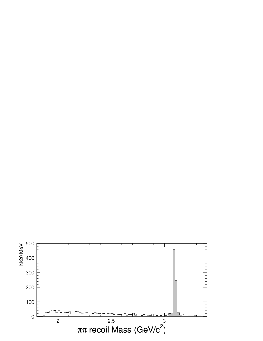
FIG. 8.: Distribution of $\pi^{+}\pi^{-}$ recoil masses in the $\Delta^{++}$ analysis. A cut is made at $\left|M_{p\overline{p}}-M_{J/\psi}\right|>60~{}\mbox{MeV}/c^{2}$ to remove $J/\psi$ contamination.

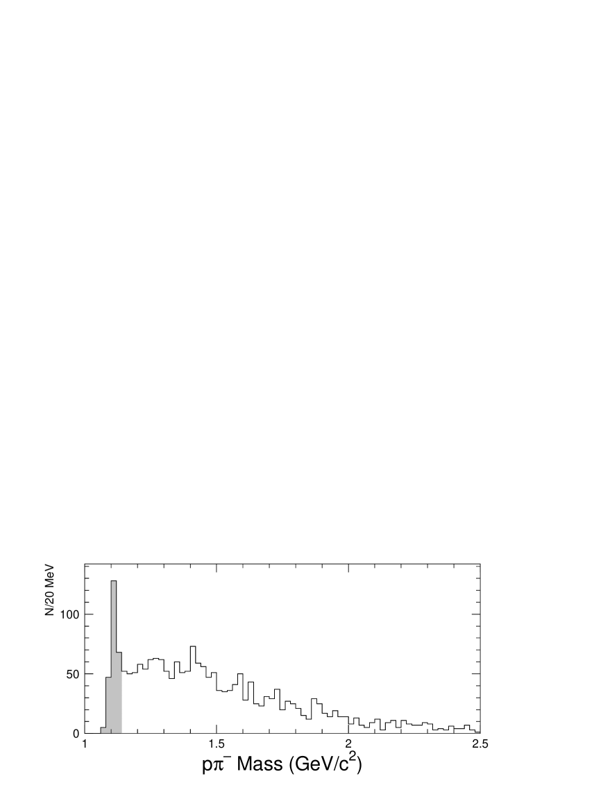
FIG. 9.: Distribution of $p\pi^{-}$ masses in the $\Delta^{++}$ analysis. A cut is made at $M_{p\pi^{-}}>1.14$ GeV$/c^{2}$ to remove $\Lambda\overline{\Lambda}$ background.

Events which pass all above cuts are fit to a spin-1 Breit-Wigner plus a 4-body phase-space background histogram. The width and centroid of the signal spectrum are fixed to the PDG[7] values. Figure 10 shows the output of the fit; there are 849 total events in the plot. The fit parameter varied is the relative proportions of the phase space background and the Breit-Wigner signal to the total number of events in the plot. $N_{\mathstrut\Delta^{++}\overline{\Delta}{}^{--}}$ is $157\pm 13\pm 34$.

FIG. 10.: Distribution of $p\pi^{+}$ masses from a kinematic fit to $\psi(2S)\to p\overline{p}\pi^{+}\pi^{-}$. Data is fit to a spin-1 Breit-Wigner plus a 4-body phase-space background (from Monte Carlo). Black boxes with error bars are data, smooth curve is the spin-1 Breit-Wigner fit result, and histogram is the final fit to background plus Breit-Wigner, binned to match the data. $N_{\Delta^{++}\overline{\Delta}{}^{--}}=157\pm 13\pm 34$.

B $\psi(2S)\to\Sigma^{+}(1385)\overline{\Sigma}{}^{-}(1385)$

The hyperons from $\psi(2S)\to\Sigma^{*+}\overline{\Sigma}{}^{*-}$ decay via $\Sigma^{+}(1385)\to\Lambda\pi^{+}$ 88% of the time. We consider only those decays where the daughter $\Lambda$s decay via the charged $p\pi$ mode. The experimental signature is $\psi(2S)\to p\overline{p}2(\pi^{+}\pi^{-})$ where one each of the $p\pi^{-}$ ($\overline{p}\pi^{+}$) candidates is consistent with being from the decay of a $\Lambda$ ($\overline{\Lambda}$).

We select events with six and only six well reconstructed tracks with a zero net charge, and in the fiducial region covered by the drift chamber, $\left|\cos\theta\right|\leq 0.80$. We kinematically fit the 36 possible charge combinations of $(+-)+(-+)-$, running the $(+-)/(-+)$ candidates through a displaced vertex finding algorithm, to $p\pi^{-}\pi^{+}\overline{p}\pi^{+}\pi^{-}$. No constraints are placed on the $(+-)/(-+)$ candidates.

Figure 11 shows that the fit mass of the daughter $\Lambda$s from the decay of the primary $\Sigma^{*+}$ is well defined and centered at the $\Lambda$ mass. We make a loose cut of 15 MeV$/c^{2}$ on the $\Lambda$ and $\overline{\Lambda}$ resonances, indicated by the arrows on the plot.

FIG. 11.: Distribution of $M_{p\pi^{-}}$ from a fit to $\psi(2S)\to$ $(p\pi^{-})\pi^{+}(\overline{p}\pi^{+})\pi^{-}$, showing the $\Lambda$ peak in $\Sigma(1385)^{+}\overline{\Sigma}(1385){}^{-}$ candidate events.

As shown in Figure 12, the mass recoiling against the orphan $\pi^{+}\pi^{-}$ pair is dominated by a peak at the $J/\psi$ mass, indicating contamination of $\psi(2S)\to\pi^{+}\pi^{-}J/\psi$, $J/\psi\to\Lambda\overline{\Lambda}$. We therefore remove events with a $\pi^{+}\pi^{-}$ recoil mass within 30 MeV$/c^{2}$ of the $J/\psi$.

FIG. 12.: Distribution of $\pi^{+}\pi^{-}$ recoil masses from a kinematic fit to $\psi(2S)\to\Lambda\overline{\Lambda}\pi^{+}\pi^{-}$, showing large $J/\psi$ contamination in $\Sigma(1385)^{+}\overline{\Sigma}(1385){}^{-}$ candidate events.

To determine $N_{\mathstrut\Sigma^{*+}\overline{\Sigma}{}^{*-}}$, we constrain the $\overline{p}\pi^{+}\pi^{-}$ combination ($\overline{\Sigma}{}^{*-}$ candidate) to be within 107.4 MeV$/c^{2}$ ($3\times\Gamma$) of the nominal PDG value in order to enhance the $\Sigma^{*+}$ signal. Events which pass the above cuts are fit to a Breit-Wigner with a constant background, with the mass and width fixed to the PDG values ($M=1382.8~{}\mbox{GeV}/c^{2}$, $\Gamma=35.8~{}\mbox{MeV}/c^{2}$). This fit is shown in Figure 13; from the fit, $N_{\mathstrut\Sigma^{*+}\overline{\Sigma}{}^{*-}}=13.8\pm 3.7\pm 2.7$.

FIG. 13.: Distribution of $M_{p\pi^{-}\pi^{-}}$ from a kinematic fit to $\psi(2S)\to(p\pi^{-})\pi^{-}(\overline{p}\pi^{+})\pi^{+}$. The histogram is an unbinned fit to a Breit-Wigner constrained to the nominal $\Sigma(1385)^{+}$ mass and width.

C $\psi(2S)\to\Xi^{0}(1530)\overline{\Xi}{}^{0}(1530)$

In the decay $\psi(2S)\to\Xi^{*}\overline{\Xi}{}^{*}$, the $\Xi^{*}$s are produced back to back in the $\psi(2S)$ rest frame. The dominant decay mode of $\Xi^{*}$ baryons is $\Xi^{*}\to\Xi^{-}\pi^{+}$, with a branching fraction of 0.66.[7] The $\Xi^{-}$ decays as in Section III D to $\Lambda\pi^{-}$, and the $\Lambda$ decays to $p\pi^{-}$.

We select events with eight and only eight well reconstructed tracks with zero net charge, and in the fiducial region covered by the drift chamber, $\left|\cos\theta\right|\leq 0.80$. Remaining events are subjected to a 4-constraint kinematic fit to the hypothesis $\psi(2S)\to p\pi^{-}\overline{p}\pi^{+}\pi^{+}\pi^{-}\pi^{+}\pi^{-}$. The $p\pi$ candidates for $\Lambda$s are sent through a displaced vertex finder. Events which pass the fit with a fit probability greater than 0.01 are examined further.

As the dominant decay mode in $\Xi^{*}$ decays includes a $\Lambda$ in the decay chain, a loose cut is placed on the $p\pi^{-}$ mass ($|M_{p\pi^{-}}-M_{\Lambda}|<20~{}\mbox{MeV}/c^{2}$) to enhance the signal fraction (Figure 14). Due to $\pi$ combinatorics, each event that passes the kinematic fit is counted four times in this plot.

FIG. 14.: Distribution of $p\pi^{-}$ masses from a kinematic fit to $\psi(2S)\to p\overline{p}\pi^{+}\pi^{-}\pi^{+}\pi^{-}\pi^{+}\pi^{-}$ showing the $\Lambda$ peak in $\Xi{}^{0}(1530)\overline{\Xi}{}^{0}(1530)$ candidate events.

Similarly, as there is a $\Xi^{-}$ in the decay chain, a cut is made on the $p\pi^{-}\pi^{-}$ invariant mass; $M_{p\pi^{-}\pi^{-}}$ is required to be within 20 MeV$/c^{2}$ of the nominal mass of the $\Xi^{-}$, as shown in Figure 15. Due to $\pi$ combinatorics, each event is counted twice in this plot.

FIG. 15.: Distribution of $p\pi^{-}\pi^{-}$ masses from a kinematic fit to $\psi(2S)\to p\overline{p}\pi^{+}\pi^{-}\pi^{+}\pi^{-}\pi^{+}\pi^{-}$, showing the $\Xi^{-}$ peak in $\Xi(1530){}^{0}\overline{\Xi}(1530){}^{0}$ candidate events.

All events which remain after the above cuts are graphed in Figure 16 with $M_{\overline{p}\pi^{+}\pi^{+}\pi^{-}}$ on the vertical axis and $M_{p\pi^{-}\pi^{-}\pi^{+}}$ on the horizontal. The signal region is shown as a circle at (1.531,1.531). No events fall within the signal region defined as a 50 MeV$/c^{2}$ radius from the central value. We set an upper limit of 2.3 events at 90% CL for $N_{\mathstrut\Xi^{*}\overline{\Xi}{}^{*}}$.

FIG. 16.: Distribution of $M_{\overline{p}\pi^{+}\pi^{+}\pi^{-}}$ vs $M_{p\pi^{-}\pi^{-}\pi^{+}}$ from a kinematic fit to the final state $\psi(2S)\to p\overline{p}\pi^{+}\pi^{-}\pi^{+}\pi^{-}\pi^{+}\pi^{-}$. The circle denotes the signal region, 3 sigma from the nominal mass of the $\Xi(1530)^{0}$.

D $\psi(2S)\to\Omega^{-}\overline{\Omega}{}^{+}$

The dominant $\Omega^{-}$ decay chain is $\Omega^{-}\to\Lambda K^{-}$, $\Lambda\to p\pi^{-}$ with a total branching fraction of 43% [7]. We look for $\psi(2S)\to\Omega^{-}\overline{\Omega}{}^{+}$ events with the topology $\psi(2S)\to p\overline{p}\pi^{+}\pi^{-}K^{+}K^{-}$, i.e. six charged tracks where the $p\pi^{-}$ and $\overline{p}\pi^{+}$ are consistent with being from the decay of a $\Lambda$ or $\overline{\Lambda}$.

We select events with six charged tracks in the polar angle region $\left|\cos\theta\right|\leq 0.8$ and with zero net charge. The remaining events are subjected to a 7-constraint kinematic fit to the hypothesis $\psi(2S)\to\Lambda\overline{\Lambda}K^{+}K^{-}$, $M_{\Lambda K^{-}}=M_{\overline{\Lambda}K^{+}}$. The fit is applied for each of the 36 particle assignment possibilities. Only the assignment with the best probability in the kinematic fit is considered.

Figure 17 shows the $\Lambda K^{-}$ mass distribution for the selected events, where the solid line histogram is data and the crosses are from Monte Carlo, normalized to three events. There are no candidates within three sigma of the nominal $\Omega^{-}$ peak, thus an upper limit of 2.3 is assigned at the 90 percent confidence level.

FIG. 17.: Distribution of $\Lambda K^{-}$ masses from a kinematic fit to $\psi(2S)\to\Lambda\overline{\Lambda}K^{+}K^{-}$. Histogram is candidate $\Omega^{-}\overline{\Omega}{}^{+}$ events, crosses are Monte Carlo.

V Continuum background

A few percent of the hadronic events in our data sample originate from non-resonant $e^{+}e^{-}\to q\overline{q}$ annihilation events. We use a 5.1 pb^-1 data sample taken off resonance to determine the level of continuum $e^{+}e^{-}\to B_{i}\overline{B_{i}}$ contamination to our event samples. We find no events that survive the analysis procedures and event selection criteria identical to those described above for either of the modes $\Lambda\overline{\Lambda}$ or $\Delta^{++}\overline{\Delta}{}^{--}$. We conclude that continuum events comprise a negligibly small contamination to our data samples.

VI Determination of the total number of $\psi(2S)$ events

We determine the number of $\psi(2S)$ events in our data samples from the observed number of cascade decays of the type $\psi(2S)\to\pi^{+}\pi^{-}J/\psi$, $J/\psi\to X$. The pions are reconstructed, and the recoil mass of the two pions is fit to determine the total number of $\psi(2S)\to\pi^{+}\pi^{-}J/\psi$ events. From this fit, the total number of these events corrected for detection efficiency is $1.227\pm 0.003\pm 0.017\times 10^{6}$. The analysis for this is documented in reference [10].

The total number of $\psi(2S)$ events is determined by dividing the number of events in the previous paragraph by the PDG branching fraction for the mode $\psi(2S)\to\pi^{+}\pi^{-}J/\psi$ [7]. This number is determined to be $3.95\pm 0.36\times 10^{6}$ where the error is dominated by the error on the $\psi(2S)\to\pi^{+}\pi^{-}J/\psi$ branching fraction [11].

VII Acceptance and Efficiency

A $p\overline{p}$

We determine the efficiency for $\psi(2S)\to p\overline{p}$ events from a sample of Monte Carlo simulated events. Events were generated with a distribution of

$$\frac{dN}{d\cos\theta}\propto 1+\alpha\cos^{2}\theta$$

with $\alpha=0.61\pm 0.23$. This proportionality constant was measured in the $J/\psi\to p\overline{p}$ system by the Mark II collaboration[8] and by the DM2 collaboration[9]. Out of 20000 events generated, 14857 events survive these cuts, yielding a general efficiency of 0.743. The collinearity cut is also purely geometric, and has an efficiency of 0.999.

As the BES Monte Carlo is of limited usefulness for simulating detailed hadronic interactions, cuts which are affected by such must be corrected for by the examination of real data. Fortunately, there is a subset of events which allow the effects of these cuts to be determined. A clean sample of $p\overline{p}$ pairs was aquired from the analysis of $\Delta^{++}\overline{\Delta}{}^{--}$ in Section IV A. The $J/\psi$ contamination shown in Figure 8 is the origin of this sample. These events are used to determine the $E_{SC}$, and $dE/dx$ cut efficiencies.

This study is summarized in Table I. The systematic error was determined from both Monte Carlo statistics and variation of cuts. The product of all efficiencies is: $0.234\pm 0.022$.

Cut	$\epsilon_{\rm MC}$	$\epsilon_{J/\psi}$	$\delta\epsilon$	$\delta{\cal B},{\rm eff}$	$\delta{\cal B},{\rm total}$
General	0.743		0.006	$0.3\times 10^{-5}$	$0.3\times 10^{-5}$
Muon ID	0.696		0.007	$0.2\times 10^{-5}$	$0.2\times 10^{-5}$
BSC Geom	0.768		0.009	$0.3\times 10^{-5}$	$0.3\times 10^{-5}$
$E_{SC}<0.7$		0.610	0.048	$1.8\times 10^{-5}$	$1.8\times 10^{-5}$
$|XSP|<3$		0.968	0.047	$1.1\times 10^{-5}$	$1.2\times 10^{-5}$
Collinearity	0.999		0.001	$0.02\times 10^{-5}$	$0.02\times 10^{-5}$

TABLE I.: Relative efficiencies and systematic errors for cuts in the mode $\psi(2S)\to p\overline{p}$ as modeled by Monte Carlo for geometric efficiencies and $J/\psi$ data for PID efficiencies. Last column includes combined systematic error due to variation of cuts.

B $\Lambda\overline{\Lambda}$, $\Sigma^{0}\overline{\Sigma}{}^{0}$, and $\Xi^{-}\overline{\Xi}{}^{+}$

We determine the efficiency for the hyperon-pair channels completely from Monte Carlo simulated events. Here we generated 20000 events in each mode with a $1+\alpha_{d}\cos\theta$ distribution, $\alpha_{d}=0.67\pm 0.21$, $0.22$, $0.5\pm 0.5$ for $\Lambda\overline{\Lambda}$, $\Sigma^{0}\overline{\Sigma}{}^{0}$, and $\Xi^{-}\overline{\Xi}{}^{+}$ respectively. The value of $\alpha_{d}$ was not varied for the $\Sigma^{0}\overline{\Sigma}{}^{0}$ mode as the statistical error was large. The values for $\alpha_{d}$ are those determined by the Mark II collaboration[8] and by the DM2 collaboration[9].

The resulting efficiencies are summarized in Table II. The systematic error reported is a combination of Monte Carlo statistics and variation of $\alpha_{d}$. Also, an additional 10 percent error is added because of uncertainties in the kinematic fitter used in these analyses.

In these three modes, we require two $\Lambda$’s that decay to charged $p\pi$ final states, which have a branching fraction ${\cal B}(\Lambda\to p\pi^{-})=0.639\pm 0.005$; the other decay modes that are required are very nearly unity, namely ${\cal B}(\Sigma\to\Lambda\gamma)=1.0$ and ${\cal B}(\Xi^{-}\to\Lambda\pi^{-})=0.999$ [7]. The branching fraction acceptance for each channel is the $\Lambda\to p\pi^{-}$ branching fraction squared: $0.41\pm 0.01.$

mode	$N_{evt}$	efficiency	B.F. Acceptance	KFit
$p\overline{p}$	$201\pm 14\pm 21$	$0.227\pm 0.032$	$1.00$
$\Lambda\overline{\Lambda}$	$80\pm 9\pm 4$	$0.27\pm 0.01$	$0.41\pm 0.01$	10%
$\Sigma^{0}\overline{\Sigma}{}^{0}$	$8\pm 3\pm 2$	$0.043\pm 0.003$	$0.41\pm 0.01$	10%
$\Xi^{-}\overline{\Xi}{}^{+}$	$12\pm 3.4\pm 0.2$	$0.078\pm 0.01$	$0.41\pm 0.01$	10%
$\Delta^{++}\overline{\Delta}{}^{--}$	$157\pm 13\pm 34$	$0.31\pm 0.02$	$1.0\pm 0.01$	10%
$\Sigma^{*+}\overline{\Sigma}{}^{*-}$	$14\pm 4\pm 3$	$0.104\pm 0.005$	$0.316\pm 0.011$	10%
$\Xi^{*0}\overline{\Xi}{}^{*0}$	$<2.3$	$0.041\pm 0.001$	$0.172\pm 0.001$	10%
$\Omega^{-}\overline{\Omega}{}^{+}$	$<2.3$	$0.042\pm 0.001$	$0.187\pm 0.001$	10%

TABLE II.: Number of events, efficiencies, branching fraction acceptances, additional systematic errors due to the kinematic fit for $\psi(2S)\to B_{i}\overline{B_{i}}$.

C Acceptance and Efficiency of the Decuplet Pairs

We determine the efficiency for the decuplet hyperon-pair channels completely from Monte Carlo simulated events. Here we generated 20000 events in each mode with a $1+\alpha_{d}\cos\theta$ distribution, $\alpha_{d}$ varying between 0 and 1 for $\Delta^{++}\overline{\Delta}{}^{--}$, and constant at 0.6 for the other modes. The resulting efficiencies are summarized in Table II, where the systematic error reported is a combination of Monte Carlo statistics and variation of $\alpha_{d}$. Also, an additional 10 percent error is added because of uncertainties in the kinematic fitter used in these analyses.

The branching fraction for $\Delta^{++}\to\pi^{+}\pi^{+}$ is greater than 0.99 [7], thus the branching fraction acceptance used is $1.00\pm 0.01$. The $\Sigma^{*+}\overline{\Sigma}{}^{*-}$ decay contains two $\Lambda$s going to $p\pi$ ($0.639^{2}$) and two $\Sigma^{*}$s decaying to $\Lambda\pi$ ($0.88^{2}$), for a total acceptance of $0.316\pm 0.011$. The $\Xi^{*0}\overline{\Xi}{}^{*0}$ decay has 3 components to the acceptance: $\Xi^{*0}\to^{-}\pi^{+}$ ($0.650^{2}$), $\Xi^{-}\to\Lambda\pi^{-}$ ($0.999^{2}$) $\Lambda\to p\pi^{-}$ ($0.639^{2}$), with a total acceptance of $0.172\pm 0.001$, and $\Omega^{-}\overline{\Omega}{}^{+}$ has only two components in the acceptance, $\Omega^{-}\to\Lambda K^{-}$ ($0.678^{2}$) and $\Lambda\to p\pi^{-}$ ($0.639^{2}$), with a total acceptance of $0.187\pm 0.001$.

VIII Results

The branching ratios ${\cal B}(\psi(2S)\to B_{i}\overline{B_{i}})/{\cal B}(\psi(2S)\to J/\psi\pi^{+}\pi^{-})$ are calculated by dividing the number of events in each mode, corrected for efficiency and branching fraction acceptance, by the corrected number of events in the reference mode, as noted in Section VI. The final branching fractions are determined by multiplying the above branching ratios by the PDG value for ${\cal B}(\psi(2S)\to J/\psi\pi^{+}\pi^{-})$, $0.310\pm 0.028$. These are shown along with the branching ratios in Table III.

We compare our results for the branching fractions to previous limits and results in Figure 18. Our measured value for the ${\cal B}(\psi(2S)\to p\overline{p})$ is about one standard deviation higher than the previous DASP measurements, which was based on 4 events [3] and a Mark I measurement with similar statistics [4]. The results for $\Lambda\overline{\Lambda}$ and $\Xi^{-}\overline{\Xi}{}^{-}$ are within the PDG upper limit values. There are no previous experimental results for $\Sigma^{0}\overline{\Sigma}{}^{0}$ or any of the decuplet modes.

mode	$N_{evt}$, Corr	${\cal B}(B_{i}\overline{B_{i}})/{\cal B}(J/\psi\pi^{+}\pi^{-})~{}(\times 10^{-4})$	${\cal B}(\times 10^{-5})$
$p\overline{p}$	$856\pm 60\pm 119$	$6.98\pm.49\pm.97$	$21.6\pm 1.5\pm 3.6$
$\Lambda\overline{\Lambda}$	$718\pm 80\pm 84$	$5.85\pm.65\pm.69$	$18.1\pm 2.0\pm 2.7$
$\Sigma^{0}\overline{\Sigma}{}^{0}$	$456\pm 162\pm 152$	$3.7\pm 1.3\pm 1.2$	$12\pm 4\pm 4$
$\Xi^{-}\overline{\Xi}{}^{+}$	$371\pm 108\pm 49$	$3.0\pm.9\pm.4$	$9.4\pm 2.7\pm 1.5$
$\Delta^{++}\overline{\Delta}{}^{--}$	$506\pm 40\pm 127$	$4.12\pm.33\pm 1.04$	$12.8\pm 1.0\pm 3.4$
$\Sigma^{*+}\overline{\Sigma}{}^{*-}$	$419\pm 113\pm 97$	$3.4\pm.9\pm.8$	$11\pm 3\pm 3$
$\Xi^{*0}\overline{\Xi}{}^{*0}$	$<322$	$<2.6$	$<8.1$
$\Omega^{-}\overline{\Omega}{}^{+}$	$<290$	$<2.4$	$<7.3$

TABLE III.: Numbers of events corrected for efficiency and branching fraction acceptance, branching fraction ${\cal B}(\psi(2S)\to B_{i}\overline{B_{i}})/$${\cal B}(\psi(2S)\to J/\psi\pi^{+}\pi^{-})$ and final branching ratios for ${\cal B}(\psi(2S)\to B_{i}\overline{B_{i}})$. Column 3 is calculated by dividing the corrected number of events in each mode by the corrected number of events in the reference mode.

FIG. 18.: Comparison of measured branching fractions (circles) with previous measurements (triangles). Two previous measurements are upper limits.

In Fig. 19, we plot the reduced branching fractions derived from our measurements. The results show a trend to smaller values for the higher massses, similar to that seen for the $J/\psi$ and are only marginally consistent with expectations from flavor-$SU(3)$ symmetry. Higher precision measurements both for the $J/\psi$ and $\psi(2S)$ would clarify this issue.

FIG. 19.: The reduced branching fractions $\left|M_{i}\right|^{2}=$ ${\cal B}(\psi(2S)\to B_{i}\overline{B_{i}})/(\pi p^{*}/\sqrt{s})$ for $\psi(2S)\to B_{i}\overline{B_{i}}$ decays.

A comparison to the perturbative QCD predictions of Bolz and Kroll [5] is shown in Figure 20. The results match quite well with these calculations.

FIG. 20.: Comparison of ${\cal B}(\psi(2S)\to B_{i}\overline{B_{i}})$ to Bolz and Kroll’s predictions from perturbative QCD. Horizontal line is $\Gamma_{exp}/\Gamma_{qcd}=1.0$.

Our measured $\psi(2S)$ branching fractions agree with expectations derived from the application of the 12% rule to the PDG values for the corresponding $J/\psi$ decays for the modes $p\overline{p}$, $\Lambda\overline{\Lambda}$, $\Sigma^{0}\overline{\Sigma}{}^{0}$ $\Xi^{-}\overline{\Xi}{}^{-}$, $\Delta^{++}\overline{\Delta}{}^{--}$ and $\Sigma^{*-}\overline{\Sigma}{}^{*+}$, as shown in Table IV and in Figure 21. There are no results for $J/\psi\to\Xi^{0}(1530)\overline{\Xi}{}^{0}(1530)$ and $J/\psi\to\Omega^{-}\overline{\Omega}{}^{+}$ is not kinematically allowed.

Decay Mode		$\cal B$	$0.116\times{\cal B}$ ($\times 10^{-5}$)
$J/\psi$$\to$	$p\overline{p}$	$(2.14\pm 0.10)\times 10^{-3}$	$24.8\pm 1.2$
$J/\psi$$\to$	$\Lambda\overline{\Lambda}$	$(1.35\pm 0.14)\times 10^{-3}$	$15.7\pm 1.7$
$J/\psi$$\to$	$\Sigma^{0}\overline{\Sigma}{}^{0}$	$(1.3\pm 0.2)\times 10^{-3}$	$15.\pm 2.$
$J/\psi$$\to$	$\Xi^{-}\overline{\Xi}{}^{+}$	$(0.9\pm 0.2)\times 10^{-3}$	$10.\pm 2.$
$J/\psi$$\to$	$\Delta^{++}\overline{\Delta}{}^{--}$	$(1.10\pm 0.29)\times 10^{-3}$	$12.8\pm 3.$
$J/\psi$$\to$	$\Sigma^{*+}\overline{\Sigma}{}^{*-}$	$(1.03\pm 0.13)\times 10^{-3}$	$11.9\pm 01.5$

TABLE IV.: Branching ratio predictions for $\psi(2S)$.

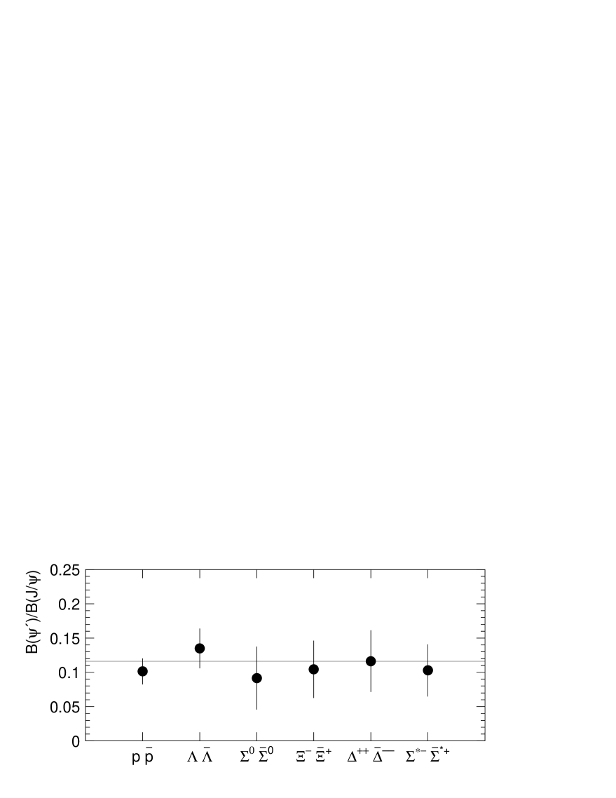
FIG. 21.: The ratio ${\cal B}(\psi(2S)\to B_{i}\overline{B_{i}})/{\cal B}(J/\psi\to B_{i}\overline{B_{i}})$. Horizontal Line is the 12 percent ratio expected from factorizing the $\psi(2S)\to B_{i}\overline{B_{i}}$ Feynman diagram.

IX Conclusions

We report measurements of the branching fractions for $\psi(2S)\to p\overline{p},~{}\Lambda\overline{\Lambda},~{}\Sigma^{0}\overline{\Sigma}{}^{0}$, $\Xi^{-}\overline{\Xi}{}^{+}$, $\Delta^{++}\overline{\Delta}{}^{--}$ and $\Sigma{}^{+}(1385)\overline{\Sigma}{}^{-}(1385)$, along with upper limits for the decays $\psi(2S)\to\Xi^{0}(1530)\overline{\Xi}{}^{0}(1530)$ and $\Omega^{-}\overline{\Omega}{}^{+}$. The measured branching fractions agree with expectations based on an application of the 12% rule to the corresponding $J/\psi$ decays. The reduced branching fractions decrease with increasing baryon masses, showing some deviation from expectations based on flavor-$SU(3)$ symmetry.

X Acknowledgements

The BES collaboration acknowledges financial support from the Chinese Academy of Sciences, the National Natural Science Foundation of China, the U.S. Department of Energy and the Ministry of Science & Technology of Korea. It thanks the staff of BEPC for their hard efforts. This work is supported in part by the National Natural Science Foundation of China under contracts Nos. 19991480 and 19825116 and the Chinese Academy of Sciences under contract No. KJ 95T-03(IHEP); by the Department of Energy under Contract Nos. DE-FG03-92ER40701 (Caltech), DE-FG03-93ER40788 (Colorado State University), DE-AC03-76SF00515 (SLAC), DE-FG03-91ER40679 (UC Irvine), DE-FG03-94ER40833 (U Hawaii), DE-FG03-95ER40925 (UT Dallas); and by the Ministry of Science and Technology of Korea under Contract KISTEP I-03-037(Korea).

REFERENCES

[1]
is calculated using the method given by the Particle Data
Group [7], with . The ratio
is calculated to be about 0.8 by
this method.
[2]
M.E.B. Franklin et al. (Mark II Collaboration),
Phys. Rev. Lett. 51, 963 (1983).
[3]
R. Brandelick et al. (DASP Collaboration), Z. Phys. C1, 233 (1979).
[4]
G. Feldman and M. Perl (Mark I Collaboration),
Phys. Rep. C33, 285 (1977).
[5]
J. Bolz and P. Kroll, Eur. Phys. J. C2, 545, (1998),
hep-ph/9703252.
[6]
J.Z. Bai et al. (BES Collaboration), Nucl. Inst. and Meth. A344,
319 (1994).
[7]
D.E. Groom et al, Review of Particle Physics, Euro. Phys. Jnl.
C15 (2000).
[8]
M.W. Eaton et al. (Mark II Collaboration), Phys. Rev. D29, 804 (1984).
[9]
D. Pallin et al. (DM2 Collaboration), Nucl. Phys. B292, 653, (1987).
[10]
J.Z. Bai et al. (BES Collaboration), Phys. Rev. D58:092006 (1998),
hep-ex/9806012.
[11]
The number of quoted in [10] has been rescaled by
1.045 to account for the change in
from PDG1996 to PDG2000.