Lattice study on kaon nucleon scattering length in the $I=1$ channel

Abstract

Using the tadpole improved clover Wilson quark action on small, coarse and anisotropic lattices, $KN$ scattering length in the $I=1$ channel is calculated within quenched approximation. The results are extrapolated towards the chiral and physical kaon mass region. Finite volume and finite lattice spacing errors are also analyzed and a result in the infinite volume and continuum limit is obtained which is compatible with the experiment and the results from Chiral Perturbation Theory.

1 Introduction

Anisotropic lattices and improved actions have been extensively used in recent lattice QCD calculations. In our previous works, the following tadpole improved gluonic action on anisotropic lattices has been utilized:

$$S= - \beta\sum_{i>j}\left[{5\over 9}{TrP_{ij}\over\xi u^{4}_{s}}-{1\over 36}{TrR_{ij}\over\xi u^{6}_{s}}-{1\over 36}{TrR_{ji}\over\xi u^{6}_{s}}\right]$$ (1)

$$- \beta\sum_{i}\left[{4\over 9}{\xi TrP_{0i}\over u^{2}_{s}}-{1\over 36}{\xi TrR_{i0}\over u^{4}_{s}}\right]\;\;,$$

where $P_{0i}$ and $P_{ij}$ represents the usual temporal and spatial plaquette variable, respectively. $R_{ij}$ and $R_{i0}$ designates the $2\times 1$ spatial and temporal Wilson loops, where, in order to eliminate the spurious states, we have restricted the coupling of fields in the temporal direction to be within one lattice spacing. The parameter $u_{s}$, which is taken to be the fourth root of the average spatial plaquette value, implements the tadpole improvement. With the tadpole improvement factor, the renormalization of the anisotropy (or aspect ratio) $\xi=a_{s}/a_{t}$ would be small. In this work, we will not differentiate the bare aspect ratio and the renormalized one in this work. Using this action, glueball and hadron spectra have been studied within quenched approximation [1, 2, 3, 4, 5, 6, 7]. In our previous works, configurations generated from this improved action have also been utilized to calculate the $\pi\pi$ scattering lengths in the $I=2$ channel [8]. In this paper, we extend our study to the kaon nucleon scattering lengths within quenched approximation. Unlike the case in pion pion scattering where the chiral expansion is quite reliable, chiral predictions in $KN$ scattering suffer from large corrections [9, 10, 11, 12]. On the experimental side, Martin used dispersion relation fits to determine the $KN$ scattering parameters [13]. Therefore, a lattice QCD calculation will offer an important and independent check on these results.

Lattice calculations of hadron scattering lengths have been performed by various authors using conventional Wilson fermions on symmetric lattices without the improvement [14, 15, 16]. In Ref. [15], a systematic study of the hadron scattering was performed, including pion-pion, kaon-nucleon, pion-nucleon and nucleon-nucleon scattering. However, this study was done only at some specific parameters and the results were not extrapolated towards the continuum and chiral limit. In later works, chiral and continuum limit was studied systematically in the case of pion-pion scattering, especially in the $I=2$ channel [16, 8, 17, 18] It is known that, using the symmetric lattices and Wilson action, large lattices have to be simulated which require substantial amount of computing resources. In Ref. [8], we have shown that, pion-pion scattering lengths can be obtained using relatively small lattices with the help of tadpole improved Wilson quarks on anisotropic lattices. It is also possible to perform the chiral, infinite volume and continuum limits extrapolation. The final extrapolated result on the pion-pion scattering length in the $I=2$ channel is in good agreement with Chiral perturbation result, the experimental result and other lattice results using conventional Wilson fermions [17]. In this paper, similar techniques are applied and the kaon-nucleon scattering lengths in the $I=1$ channel is studied.

The fermion action used in this study is the tadpole improved clover Wilson action on anisotropic lattices [19, 20, 8]:

$${\mathcal{M}}_{xy} = \delta_{xy}\sigma+{\mathcal{A}}_{xy}$$

$${\mathcal{A}}_{xy} = \delta_{xy}\left[{1\over 2\kappa_{\max}}+\rho_{t}\sum^{3}_{i=1}\sigma_{0i}{\mathcal{F}}_{0i}+\rho_{s}(\sigma_{12}{\mathcal{F}}_{12}+\sigma_{23}{\mathcal{F}}_{23}+\sigma_{31}{\mathcal{F}}_{31})\right]$$ (2)

$$- \sum_{\mu}\eta_{\mu}\left[(1-\gamma_{\mu})U_{\mu}(x)\delta_{x+\mu,y}+(1+\gamma_{\mu})U^{\dagger}_{\mu}(x-\mu)\delta_{x-\mu,y}\right]\;\;,$$

where various coefficients in the fermion matrix ${\mathcal{M}}$ are given by:

$$\eta_{i} = \nu/(2u_{s})\;\;,\;\;\eta_{0}=\xi/2\;\;,\;\;\sigma=1/(2\kappa)-1/(1\kappa_{max})\;\;,$$

$$\rho_{t} = c_{SW}(1+\xi)/(4u^{2}_{s})\;\;,\;\;\rho_{s}=c_{SW}/(2u^{4}_{s})\;\;.$$ (3)

Among the parameters which appear in the fermion matrix, $c_{SW}$ is the coefficient of the clover term and $\nu$ is the so-called bare velocity of light, which has to be tuned non-perturbatively using the single pion dispersion relations [20]. Tuning the clover coefficients non-perturbatively is a difficult procedure. In this work, the tadpole improved tree-level value, namely $c_{SW}=1$, is used.

In the fermion matrix (1), the bare quark mass dependence is singled out into the parameter $\sigma$ and the matrix ${\mathcal{A}}$ remains unchanged if the bare quark mass is varied. This shifted structure of the matrix ${\mathcal{M}}$ can be utilized to solve for quark propagators at various values of valance quark mass $m_{0}$ (or equivalently $\kappa$) at the cost of solving only the lightest valance quark mass value at $\kappa=\kappa_{\max}$, using the so-called Multi-mass Minimal Residual ($M^{3}R$ for short) algorithm [21, 22, 23]. This is particularly advantageous in a quenched calculation since one needs the results at various quark mass values to perform the chiral extrapolation.

This paper is organized as follows. In Section 2, the method to calculate $KN$ scattering lengths is briefly reviewed. The $KN$ correlation functions used in our calculation are defined. In Section 3, some simulation details are described. In Section 4, our results of the $KN$ scattering lengths obtained on lattices of various sizes and lattice spacings are extrapolated towards the chiral limit. Physical strange quark mass is also determined from the $K$-input. Finite size effects are then studied and the infinite volume limit are taken. Finally, our lattice results are extrapolated towards the continuum limit. Comparisons with the experimental value and values from chiral perturbation theory at various orders are also discussed. In Section 5, we conclude with some general remarks.

2 Formulation to extract the scattering length

In order to calculate the elastic scattering lengths for hadron-hadron scattering on the lattice, or the scattering phase shifts in general, one uses Lüscher’s formula which relates the exact energy level of two hadron states in a finite box to the elastic scattering phase shift in the continuum. In the case of $KN$ scattering at zero relative three momentum, this formula amounts to a relation between the exact energy $E^{(I)}_{KN}$ of the $KN$ system in a finite box of size $L$ with isospin $I$, and the corresponding scattering length $a^{(I)}_{0}$ in the continuum. This formula reads [24]:

$$E^{(I)}_{KN}-(m_{K}+m_{N})=-\frac{2\pi a^{(I)}_{0}}{\mu_{KN}L^{3}}\left[1+c_{1}\frac{a^{(I)}_{0}}{L}+c_{2}(\frac{a^{(I)}_{0}}{L})^{2}\right]+O(L^{-6})\;\;,$$ (4)

where $c_{1}=-2.837297$, $c_{2}=6.375183$ are numerical constants and $\mu_{KN}=m_{K}m_{N}/(m_{K}+m_{N})$ is the reduced mass of the $KN$ system. In this paper, the $KN$ scattering length $a^{(1)}_{0}$ in the $I=1$ channel will be studied.

To measure the hadron mass values $m_{K}$, $m_{N}$ and to extract the energy shift $\delta E^{(1)}_{KN}$, we construct the correlation functions from the corresponding operators in the $I=1$ channel. In this work, the hadron states that need to be measured include pion, kaon, rho, nucleon and $KN$ states. The local operators which create a single pion with appropriate isospin values are:

$$\pi^{+}({\bf x},t) = -\bar{d}({\bf x},t)\gamma_{5}u({\bf x},t)\;\;,\;\;\pi^{-}({\bf x},t)=\bar{u}({\bf x},t)\gamma_{5}d({\bf x},t)\;\;,\;\;$$

$$\pi^{0}({\bf x},t) = {1\over\sqrt{2}}[\bar{u}({\bf x},t)\gamma_{5}u({\bf x},t)-\bar{d}({\bf x},t)\gamma_{5}d({\bf x},t)]\;\;,$$ (5)

where $u({\bf x},t)$, $d({\bf x},t)$, $\bar{u}({\bf x},t)$ and $\bar{d}({\bf x},t)$ are basic local quark fields corresponding to $u$ and $d$ quarks, respectively. The operators which correspond to zero momentum single pions are:

$$\pi^{a}_{0}(t)={1\over L^{3/2}}\sum_{{\bf x}}\pi^{a}({\bf x},t)\;\;,$$ (6)

where the flavor of pions $a=+,-,0$ and $L^{3}$ is the three volume of the lattice. Zero momentum one pion correlation function can then be formed:

$$C_{\pi}(t)=<\pi^{\bar{a}}_{0}(t)\pi^{a}_{0}(0)>\;\;.$$ (7)

Similarly, one can construct the kaon correlation functions from kaon operators. In the $I=1$ channel, only $K^{+}$ and proton operators are needed:

$$K^{+}({\bf x},t) = -\bar{s}({\bf x},t)\gamma_{5}u({\bf x},t)\;\;,$$

$$p({\bf x},t) = \epsilon_{abc}\left[u^{T}_{a}({\bf x},t)(C^{-1}\gamma_{5})d_{b}({\bf x},t)\right]u_{c}({\bf x},t)\;.$$ (8)

The proton operator given above is itself a Dirac spinor. The zero momentum proton-proton correlation function is obtained by projecting out the positive parity part of the zero momentum spinor operator and taking the trace in Dirac space:

$$C_{N}(t)=\sum_{{\bf x},{\bf y}}\left\langle p({\bf x},0)\left({1+\gamma_{0}\over 2}\right)p({\bf y},t)\right\rangle\;.$$ (9)

From the large $t$ behavior of the correlation functions, the pion mass $m_{\pi}$, the kaon mass $m_{K}$ and the nucleon mass $m_{N}$ are obtained.

Two hadron operators are used in the construction of two hadron correlation functions. For example, the $KN$ operator in the $I=1$ channel is given by:

$$O^{I=1}_{KN}(t)=K^{+}_{0}(t)p_{0}(t+1)\;\;,\bar{O}^{I=1}_{KN}(t)=K^{-}_{0}(t)\bar{p}_{0}(t+1)\;\;,$$ (10)

where $K^{+}_{0}(t)$ and $p_{0}(t)$ are the zero momentum kaon and proton operators respectively. From these operators, two hadron correlation functions can be constructed. The $KN$ correlation function in the $I=1$ channel reads:

$$C^{I=1}_{KN}(t)=<\bar{O}^{I=1}_{KN}(0)\left({1+\gamma_{0}\over 2}\right)O^{I=1}_{KN}(t)>\;\;.$$ (11)

Numerically, it is more advantageous to construct the ratio of the correlation functions defined above:

$${\mathcal{R}}^{I=1}(t)=C^{I=1}_{KN}(t)/(C_{K}(t)C_{N}(t))\;\;.$$ (12)

This ratio thus exhibits the following asymptotic behavior for large $t$:

$${\mathcal{R}}^{I=1}(t)\stackrel{{\scriptstyle t>>1}}{{\sim}}e^{-\delta E^{(1)}_{KN}t}\;\;,$$ (13)

with $\delta E^{(1)}_{KN}=E^{(1)}_{KN}-m_{K}-m_{N}$ is the energy shift in this channel which directly enters Lüscher’s formula (4). This formula is utilized for small $\delta E^{(1)}_{KNi}t$ values (large enough $L$) in the calculation where the signal to noise ratio is good. In this case, one could equally use the linear fitting function:

$${\mathcal{R}}^{I=1}(t)\stackrel{{\scriptstyle T>>t>>1}}{{\sim}}1-\delta E^{(1)}_{KN}t\;\;,$$ (14)

to determine the energy shift $\delta E^{(1)}_{KN}$. Similar procedure has also been used in lattice studies of pion-pion scattering lengths by various groups.

$KN$ correlation function, or equivalently, the ratio ${\mathcal{R}}^{I=1}(t)$ constructed above can be transformed into products of quark propagators using Wick’s theorem.

Figure 1: The diagrams that contribute to $KN$ scattering in the $I=1$ channel. The solid lines represent $u$-quark propagators while dashed lines are $d$-quark propagators. The dashed-dotted lines designates the strange quark propagator. Note that diagram (b) in fact contains two different contractions.

These contributions are represented by diagrams as shown in Fig. 1, where the solid, the dashed and the dashed-dotted lines represent the $u$, $d$ and $s$ quark propagators, respectively.The $KN$ correlation function in the $I=0$ channel is, however, more complicated which involves vacuum diagrams that require to compute the quark propagators for wall sources placed at every time-slice, a procedure which is more time-consuming than in the $I=1$ channel.

3 Simulation details

Simulations are performed on a PC based cluster with $30$ nodes. Configurations are generated using the pure gauge action (1) for $6^{3}40$, $8^{3}40$ and $10^{3}50$ lattices with the gauge coupling $\beta=1.7$, $1.9$, $2.2$ and $2.4$. The spatial lattice spacing $a_{s}$ is roughly between $0.2$fm and $0.4$fm while the physical size of the lattice ranges from $1.2$fm to $4.0$fm. For each set of parameters, several hundred decorrelated gauge field configurations are used to measure the fermionic quantities. Statistical errors are all analyzed using the usual jack-knife method. Basic information of these configurations is summarized in Table 1.

Table 1: Simulation parameters for lattices studied in this work. Input aspect ratio parameter $\xi$ is fixed to be $5$ for all lattices being studied. The approximate spatial lattice spacing $a_{s}$ in physical units as obtained from [2, 7] is also indicated. Also listed are the maximum value of the hopping parameter $\kappa_{\max}$. In the last three columns, we listed the physical up/down quark hopping parameters, the physical strange quark hopping parameters and the results for the factor $F=a^{(1)}_{0}m^{2}_{\rho}/\mu_{KN}$ at physical quark mass values, respectively. In the rows labelled as ”Extrapolated”, we have also listed the values of $F$ after the infinite volume extrapolation.

Lattice	No. confs	$\kappa_{\max}$	$\kappa^{(phy)}_{u}$	$\kappa^{(phy)}_{s}$	$F=a^{(1)}_{0}m^{2}_{\rho}/\mu_{KN}$
$\beta=2.4$, $u^{4}_{s}=0.4090$, $a_{s}\simeq 0.22$fm, $\nu$=0.93
$6^{3}40$	$288$	$0.0610$	$0.06179(2)$	$0.06120(6)$	$-0.7(15)$
$8^{3}40$	$192$	$0.0610$	$0.061791(9)$	$0.06113(4)$	$-1.6(6)$
$10^{3}50$	$204$	$0.0605$	$0.061636(9)$	$0.06113(5)$	$-3.3(9)$
Infinite					$-3.3(11)$
$\beta=2.2$, $u^{4}_{s}=0.378$, $a_{s}\simeq 0.27$fm, $\nu$=0.95
$6^{3}40$	$256$	$0.0605$	$0.06116(1)$	$0.06020(2)$	$-1.9(3)$
$8^{3}40^{*}$	$224$	$0.0600$	$0.06113(1)$	$0.06041(5)$	$-3.1(9)$
$10^{3}50$	$184$	$0.0605$	$0.061230(7)$	$0.06024(2)$	$-3.3(13)$
Infinite					$-3.9(11)$
$\beta=1.9$, $u^{4}_{s}=0.3281$, $a_{s}\simeq 0.35$fm, $\nu$=0.93
$6^{3}40^{*}$	$304$	$0.0600$	$0.06087(1)$	$0.05945(2)$	$-2.3(7)$
$8^{3}40^{*}$	$160$	$0.0595$	$0.06073(1)$	$0.05969(5)$	$-2.8(46)$
$10^{3}50^{*}$	$252$	$0.0595$	$0.060722(6)$	$0.05964(2)$	$-4.0(44)$
Infinite					$-4.1(46)$
$\beta=1.7$, $u^{4}_{s}=0.295$, $a_{s}\simeq 0.39$fm, $\nu$=0.90
$6^{3}40^{*}$	$288$	$0.0590$	$0.06027(1)$	$0.05895(3)$	$-2.9(25)$
$8^{3}40^{*}$	$240$	$0.0585$	$0.06019(1)$	$0.05906(4)$	$-3.1(58)$
$10^{3}50^{*}$	$250$	$0.0580$	$0.06007(2)$	$0.05914(9)$	$-3.4(62)$
Infinite					$-4.6(64)$

Quark propagators are measured using the Multi-mass Minimal Residue algorithm for several different values of bare quark mass. Periodic boundary condition is applied to all three spatial directions while in the temporal direction, Dirichlet boundary condition is utilized. In this calculation, it is advantageous to use the wall sources which enhance the signal [14, 15, 16, 8]. Values of the maximum hopping parameter $\kappa_{\max}$, which corresponds to the lowest valance quark mass, are also listed in Table 1. Typically, a few hundred Minimal Residual iterations are needed to obtain the solution vector for a given source. On small lattices, in particular those with a low value of $\beta$, the hopping parameter has to be kept relatively far away from its critical value in order to avoid the appearance of exceptional configurations. The parameter $\nu$, also known as the bare velocity of light, that enters the fermion matrix (1) is determined non-perturbatively using the single pion dispersion relations as described in Ref. [20] and Ref. [8]. The optimal value of $\nu$ which corresponds to each parameter set of the simulation is also tabulated in Table 1

Single pion, kaon, rho and nucleon mass values are obtained from the plateau of their corresponding effective mass plots. The fitting interval is automatically chosen by minimal $\chi^{2}$ per degree of freedom. Due to the usage of finer lattice spacing in the temporal direction, good plateau behavior was observed in these effective mass plots. Therefore, contaminations from excited states should be negligible. These mass values will be utilized in the chiral extrapolation.

Figure 2: The ratio $R^{(1)}(t)$ as a function of $t$ obtained from the $KN$ correlation functions for $8$ different values of the bare quark mass. The lattice size is $8^{3}40$ and the gauge coupling $\beta=2.4$. The optimal bare velocity of light is taken to be $\nu=0.93$. The straight lines are linear fits according to Eq. (14), from which the energy shifts $\delta E\equiv E^{(1)}_{KN}-m_{K}-m_{N}$ are extracted for all possible values of $(\kappa_{u},\kappa_{s})$.

$KN$ correlation functions and the ratio ${\mathcal{R}}^{(1)}(t)$ are constructed from products of suitable quark propagators according to Wick’s theorem. Both the Direct and the Cross contributions are included. For the ratio ${\mathcal{R}}^{(1)}(t)$, we obtain clear signal for all our data sets. Since a kaon consists of one up (down) and one strange quark whose mass is different from the up and down quarks, all physical quantities involving the kaon will depend on two quark masses. In terms of the hopping parameters, the $KN$ correlation functions depends on a pair of hopping parameters: $(\kappa_{u},\kappa_{s})$. In Fig. 2 we show the ratio ${\mathcal{R}}^{(1)}(t)$ for different pairs of $\kappa$ values as a function of the temporal separation $t$, together with the corresponding linear fit (14) for $\beta=2.4$ on $8^{3}40$ lattices. The starting and ending positions of the straight lines indicate the appropriate fitting range which minimizes the $\chi^{2}$ per degree of freedom.

After obtaining the energy shifts $\delta E^{(1)}_{KN}$, these values are substituted into Lüscher’s formula to solve for the scattering length $a^{(1)}_{0}$ for all possible hopping parameter pairs: $(\kappa_{u},\kappa_{s})$, which corresponds to the up (down) and the strange bare quark mass values respectively. This is done for lattices of all sizes being simulated and for all values of $\beta$. From these results, attempts are made to perform an extrapolation towards the chiral, infinite volume and continuum limit.

4 Extrapolation towards chiral, infinite volume and continuum limits

The chiral extrapolations of physical quantities involving both the up (down) and the strange quarks consists of two steps. In the first step, the bare strange quark mass, or equivalently the corresponding hopping parameter $\kappa_{s}$, is kept fixed while the hopping parameter of the up/down quark, $\kappa_{u}$, is brought to their physical value $\kappa^{(phy)}_{u}$. The precise value of $\kappa^{(phy)}_{u}$ can be obtained by inspecting the chiral behavior of the pseudo-scalar (pion) and the vector meson (rho) mass values. In the second step, one fixes the up/down quark hopping parameter at its physical value obtained in the first step and extrapolate/interpolate in the strange quark mass. The physical strange quark hopping parameter $\kappa^{(phy)}_{s}$ is determined by demanding the mass of the kaon being exactly at its physical value ($493$MeV). In practice, this could be accomplished by, for example, inspecting the kaon to rho mass ratio. This is also known as the $K$-input. After these two steps, we would be able to obtain physical quantities at the physical up/down and strange quark mass values. In Table 1, we have listed the physical hopping parameters $\kappa^{(phy)}_{u}$ and $\kappa^{(phy)}_{s}$ for the up/down quarks and the strange quark. Note that one only needs the pion, kaon and rho correlation functions to determine the physical hopping parameters of the quarks.

We now come to the chiral extrapolation of the scattering length. In the chiral limit, the $KN$ scattering length in the $I=1$ channel is given by the current algebra result:

$$a^{(1)}_{0}=-{1\over 4\pi}{\mu_{KN}\over f^{2}_{K}}\;\;,$$ (15)

where $a^{(1)}_{0}$ is the $KN$ scattering length in the $I=1$ channel and $f_{K}\sim 113$MeV is the kaon decay constant. Chiral Perturbation Theory to one-loop order gives an expression which includes the next-to-leading order contributions [12]. Unlike the chiral perturbation theory results for the mesons, the chiral expansion for baryons also receives corrections which are suppressed by the meson to baryon mass ratios. Since the mass of the kaon is not light, one typically obtains large corrections from the next chiral order compared with the previous one. In the case of the $KN$ scattering length $a^{(1)}_{0}$, the next order correction is $114$% with the opposite sign and the next-to-next order is about $94$% with the same sign of the tree-level. This is a signal that one really has no control over the expansion.

To perform the chiral extrapolation of the scattering length, it is more convenient to use the quantity $F=a^{(1)}_{0}m^{2}_{\rho}/\mu_{KN}$, which in the chiral limit reads:

$$F\equiv{a^{(1)}_{0}m^{2}_{\rho}\over\mu_{KN}}=-{1\over 4\pi}{m^{2}_{\rho}\over f^{2}_{K}}\sim-3.686\;\;,$$ (16)

where the final numerical value is obtained by substituting in the experimental values for $m_{\rho}\sim 770$MeV and $f_{K}\sim 113$MeV. The factor $F$ can be calculated on the lattice with good precision without the lattice calculation of meson decay constants. The error of the factor $F$ obtained on the lattice will mainly come from the error of the scattering length $a^{(1)}_{0}$, or equivalently, the energy shift $\delta E^{(1)}_{KN}$ and nowhere else. Since we have calculated the factor $F$ for several different values of valance quark mass, we could make a chiral extrapolation and extract the corresponding results in the chiral limit.

First, we extrapolate the factor $F$ in the up/down quark mass values. In this step, we have adopted a simple linear extrapolation. the fitting range of the extrapolation is self-adjusted by the program to yield a minimal $\chi^{2}$ per degree of freedom. Second, the extrapolated values for the factor $F$ are then extrapolate/interpolate in the strange quark mass. Our hopping parameters are chosen such that the physical strange quark mass is either within the range of our choice or very close to avoid a long extrapolation in the strange quark mass. In Fig. 3, we have shown the two step chiral extrapolation for one of our simulation points.

Figure 3: Chiral extrapolation for the quantity $F\equiv a^{(1)}_{0}m^{2}_{\rho}/\mu_{KN}$ for our simulation results at $\beta=2.4$ on $8^{3}40$ lattices. In the lower panel, the factor $F$ as defined in Eq. (16) are plotted versus the pion mass squared, for fixed strange quark mass. The straight lines represent the corresponding linear fit in $m^{2}_{\pi}$ for the data. In the upper panel of the plot, the extrapolated quantity $F$ is plotted (open squares) as a function of strange quark mass parameter $1/(2\kappa_{s})$. The straight line represents the linear interpolation/extrapolation to the physical strange quark mass, where the result is depicted as a solid square. As a comparison, the corresponding semi-experimental result [13] for this quantity is shown as a filled circle. Chiral perturbation theory results are also shown as a filled triangle (tree), a filled square (next) and a filled hexagon (next-to-next), respectively.

In the lower panel of Fig. 3, we have plotted the results for the factor $F$ for all possible pairs of quark mass values. They are arranged according to different up/down quark hopping parameter. The straight lines show the extrapolation in $m^{2}_{\pi}$ (the first step extrapolation). The physical up/down quark hopping parameter are read from the pion and rho correlation function fits which are tabulated in Tab. 1. The resulting factor $F$ after the first extrapolation are plotted in the upper panel of Fig. 3 versus the strange quark mass parameter $1/(2\kappa_{s})$. The straight line is the linear extrapolation/interpolation (second extrapolation) and the final result is also depicted as a solid square at the physical strange quark mass. Current algebra result and the result from chiral perturbation theory are also shown as a filled triangle (tree level), a filled square (next order) and a filled hexagon (next-to-next), respectively. The result from Ref. [13] is shown as a filled circle. To avoid crowdedness, these symbols are shifted to the left. The fitting quality for the factor $F$ are reasonable. The quality for the chiral extrapolation of other simulation points are similar. As is seen, the linear fit gives a reasonable modelling of the data. The divergent contributions and other higher order corrections from quenched chiral perturbation theory seem to be numerically small for the lattices being simulated.

After the chiral extrapolation, we now turn to study the finite volume effects of the simulation. According to formula (4), the quantity $F$ obtained from finite lattices differs from its infinite volume value by corrections of the form $1/L^{3}$. However, the situation might be different in a quenched calculation, which happened in the case of pion-pion scattering [15, 25]. In the case of $KN$ scattering length, a similar calculation using quenched chiral perturbation theory is still not available. Therefore, we will be using a linear extrapolation in $1/L^{3}$, as suggested by Lüscher’s formula. In Table. 1, we have listed the infinite volume extrapolation for our simulation points at $\beta=2.4$, $2.2$, $1.9$ and $1.7$.

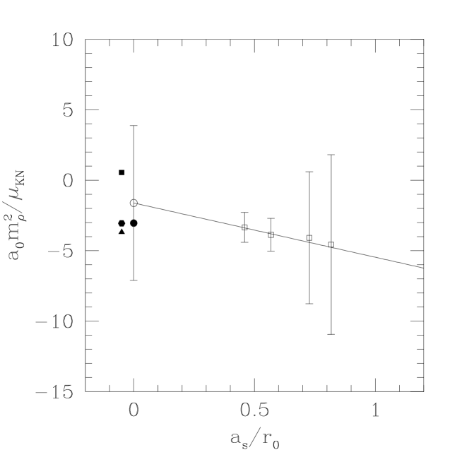
Figure 4: Continuum extrapolation for the quantity $a^{(1)}_{0}m^{2}_{\rho}/\mu_{KN}$ obtained from our simulation results at $\beta=2.4$, $2.2$, $1.9$ and $1.7$. The straight line represents the linear extrapolation in $a_{s}/r_{0}$. The extrapolated results are also shown, together with the experimental result from Ref. [13] indicated by the filled circle. For comparison, the results from Chiral perturbation theory are also shown as the points at $a_{s}=0$ respectively.

Finally, we can make an extrapolation towards the continuum limit by eliminating the finite lattice spacing errors. Since we have used the tadpole improved clover Wilson action, all physical quantities differ from their continuum counterparts by terms that are proportional to $a_{s}$. The physical value of $a_{s}$ for each value of $\beta$ can be found from Ref. [2, 7], which is also included in Table 1. This extrapolation is shown in Fig. 4 where the results from the chiral and infinite volume extrapolation discussed above are indicated as data points in the plot for all $4$ values of $\beta$ that have been simulated. The straight line shows the extrapolation towards the $a_{s}=0$ limit and the extrapolated results are also shown as solid squares together with the experimental result from Ref.[13] which is shown as the filled circle. For comparison, the results from chiral perturbation theory ar various orders are also shown as the filled triangle, the filled square and the filled hexagon at $a_{s}=0$, respectively. It is seen from the figure that our extrapolated result is negative, with a large error bar. Therefore, we can only say that, from our preliminary study we obtain a result which is compatible with the experimental result and results from chiral perturbation theory. The error of our calculation can be reduced by further studies with more statistics and on lattices with smaller lattice spacing in the future. To summarize, we obtain from the linear extrapolation the following result for the quantity $F=a^{(1)}_{0}m^{2}_{\rho}/\mu_{KN}=(-1.6\pm 5.4)$. If we substitute in the physical values, we obtain the $KN$ scattering length in the $I=1$ channel: $a^{(1)}_{0}=(-0.17\pm 0.59)\mbox{fm}$, which is to be compared with the experimental result of $(-0.33)\mbox{fm}$ and the chiral result of $(-0.398+0.457-0.389)\mbox{fm}$ at the first, second and third chiral order, respectively.

5 Conclusions

In this paper, we have calculated kaon nucleon scattering lengths in isospin $I=1$ channel using quenched lattice QCD. It is shown that such a calculation is feasible using relatively small, coarse and anisotropic lattices. The calculation is done using the tadpole improved clover Wilson action on anisotropic lattices. Simulations are performed on lattices with various sizes, ranging from $1.2$fm to about $4$fm and with four different values of lattice spacing. Quark propagators are measured with different valence quark mass values. These enable us to explore the finite volume and the finite lattice spacing errors in a systematic fashion. The infinite volume extrapolation is made. The lattice result for the scattering length is extrapolated towards the chiral and continuum limit where a result consistent with the experiment and the Chiral Perturbation Theory is found. We believe that, using the method described in this exploratory study, more reliable results on $KN$ scattering lengths could be obtained with more statistics and with simulations on finer lattices.

References

- [1] C. Morningstar and M. Peardon. Phys. Rev. D, 56:4043, 1997.
- [2] C. Morningstar and M. Peardon. Phys. Rev. D, 60:034509, 1999.
- [3] C. Liu. Chinese Physics Letter, 18:187, 2001.
- [4] C. Liu. Communications in Theoretical Physics, 35:288, 2001.
- [5] C. Liu. In Proceedings of International Workshop on Nonperturbative Methods and Lattice QCD, page 57. World Scientific, Singapore, 2001.
- [6] C. Liu and J. P. Ma. In Proceedings of International Workshop on Nonperturbative Methods and Lattice QCD, page 65. World Scientific, Singapore, 2001.
- [7] C. Liu. Nucl. Phys. (Proc. Suppl.) B, 94:255, 2001.
- [8] C. Liu, J. Zhang, Y. Chen, and J.P. Ma. Nucl. Phys. B, 624:360, 2002.
- [9] Chang-Hwan Lee, Hong Jung, Dong-Pil Min, and Mannque Rho. Phys. Lett. B, 326:14, 1994.
- [10] Martin J. Savage. Phys. Lett. B, 331:411, 1994.
- [11] Chang-Hwan Lee, G. E. Brown, Dong-Pil Min, and Mannque Rho. Nucl. Phys. A, 585:401, 1995.
- [12] N. Kaiser. Phys. Rev. C, 64:045204, 2001.
- [13] A.D. Martin. Nucl. Phys. B, 179:33, 1981.
- [14] R. Gupta, A. Patel, and S. Sharpe. Phys. Rev. D, 48:388, 1993.
- [15] M. Fukugita, Y. Kuramashi, H. Mino, M. Okawa, and A. Ukawa. Phys. Rev. D, 52:3003, 1995.
- [16] S. Aoki et al. Nucl. Phys. (Proc. Suppl.) B, 83:241, 2000.
- [17] JLQCD Collaboration. Phys. Rev. D, 66:077501, 2002.
- [18] CP-PACS Collaboration. Phys. Rev. D, 67:014502, 2003.
- [19] T. R. Klassen. Nucl. Phys. (Proc. Suppl.) B, 73:918, 1999.
- [20] Junhua Zhang and C. Liu. Mod. Phys. Lett. A, 16:1841, 2001.
- [21] A. Frommer, S. Güsken, T. Lippert, B. Nöckel, and K. Schilling. Int. J. Mod. Phys. C, 6:627, 1995.
- [22] U. Glaessner, S. Guesken, T. Lippert, G. Ritzenhoefer, K. Schilling, and A. Frommer. hep-lat/9605008.
- [23] B. Jegerlehner. hep-lat/9612014.
- [24] M. Lüscher. Commun. Math. Phys., 105:153, 1986.
- [25] C. Bernard and M. Golterman. Nucl. Phys. (Proc. Suppl.) B, 47:553, 1996.