ITEP-LAT/2003-17
August, 2003
$q\bar{q}$ and $2q2\bar{q}$ systems in terms of P-vortices

Abstract

We study the action and the energy densities of the confining string in the indirect $Z(2)$ projection of $SU(2)$ lattice gauge theory. We find that the width of the confining string is proportional to the logarithm of the distance between the quark and antiquark. In $2q2\bar{q}$ system we observe the effect of the reconstruction of the flux tube when we change the distance between two $q\bar{q}$ pairs.

1 INTRODUCTION

The structure of the confining string in terms of the Abelian or monopole operators after the Abelian projection has been studied in lattice $SU(2)$ and $SU(3)$ gluodynamics and in lattice QCD with two quark flavors [1, 2]. The distribution of the monopole currents and the electric field near the confining string is similar to the distribution of the currents of the Cooper pairs and magnetic field near the Abrikosov string [3]. Thus the quantum confining string is similar to the classical solution of the equations of motion of the Abelian Higgs model. For the center–vortex model of confinement [4] there is no corresponding classical model, confinement is due to (quasi)randomly distributed magnetic fluxes in the vacuum. On the other hand the numerical investigation of the confining string in terms of P–vortices is even simpler than that in the Abelian projection, since the statistical fluctuations are smaller [5]. In Section 2 we give the main definitions. In Section 3 we present the results of the calculations of the electric and magnetic fields near the confining string. In Section 4 we discuss the confining strings in the $2q2\bar{q}$ system.

All results are obtained on $24^{4}$ lattice at $\beta=2.40$ (20 statistically independent configurations), $\beta=2.50$ (50 configurations), and on $28^{4}$ lattice at $\beta=2.55$ (50 configurations), $\beta=2.60$ (25 configurations). To fix the physical scale we use the data for the string tension in lattice units [6] and use $\sqrt{\sigma}=440\,MeV$.

2 MAIN DEFINITIONS

To extract P–vortices we use the indirect maximal center projection defined as follows [4]. First, we fix the maximal Abelian gauge by maximizing the functional $R_{U(1)}=\sum_{x,\mu}\mathop{\rm Tr}[U_{x\mu}\sigma^{3}U_{x\mu}^{+}\sigma^{3}]$ using the simulated annealing algorithm [7]. Then we replace link matrices $U_{x\mu}$ by the Abelian link variables $U_{x\mu}\rightarrow u_{x\mu}=\frac{U_{x\mu}^{11}}{|U_{x\mu}^{11}|}$. Further gauge fixing is done by maximization of the functional $R_{Z(2)}=\sum_{x,\mu}[\Re e\;u_{x\mu}]^{2}$. Finally, the maximal center projection is performed by replacing $u_{x\mu}\rightarrow Z_{x\mu}=\mathop{\rm sign}\;\Re e\;u_{x\mu}$.

Since we are working on the symmetric lattices we have no apriori defined time axis. But when we introduce the $R\times T$ Wilson loop in the $i,4$ plane we define the time direction ($\mu=4$) and it becomes possible to define the lattice electric and magnetic field strength as follows:

$$(\vec{E}^{a}_{lat}(x))^{2}=\sum_{i=1}^{3}\left(1-P_{4i}(x)\right)\,,$$ (1)

$$(\vec{H}^{a}_{lat}(x))^{2}=\sum_{i>j}\left(1-P_{ij}(x)\right)\,,$$ (2)

where plaquette $P_{\mu\nu}(x)=\frac{1}{2}\mbox{Tr}U_{x,\mu\nu}$ in case of $SU(2)$ fields. The Euclidean action density and energy density are defined as follows:

$$\sigma(x)=(\vec{E}^{a}_{lat}(x))^{2}+(\vec{H}^{a}_{lat}(x))^{2}\,,$$ (3)

$$\varepsilon(x)=(\vec{E}^{a}_{lat}(x))^{2}-(\vec{H}^{a}_{lat}(x))^{2}\,.$$

In the $Z(2)$ projection the static quarks are represented by $Z(2)$ Wilson loop, $W_{Z(2)}$, constructed from $Z(2)$ links. $P_{\mu\nu}(x)$ entering (1), (2) are now the average of four $Z(2)$ plaquettes in the $\{\mu,\nu\}$ plain which share the site $x$. To measure the expectation value of the operator $O(x)$ in the presence of static quarks the following quantity should be calculated:

$$<O(x)>_{W}=\frac{<O(x)W>}{<W>}-<O(x)>\,,$$ (4)

where $W$ is the Wilson loop. In ref.[5] this expression was used to calculate the expectation values of $Z(2)$ plaquettes in the vicinity of the confining string.

3 NUMERICAL RESULTS

The results are presented in Figures 1 (a),(b).

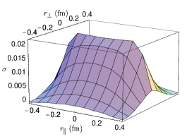
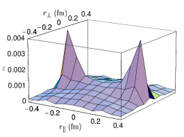
(a) (b)

Figure 1: $<\sigma(x)>_{W}$ (a) and $<\varepsilon(x)>_{W}$ (b) defined by eqs. (3), (4). Calculations are performed for $\beta=2.5$. The size of the Wilson loop is $8\times 10$.

The Coulomb peaks are not seen for the action density. For the energy density one can see rather narrow peaks which is in accordance with the result of ref. [4] where it was found that the static potential in the $Z(2)$ projection is linear down to very small distances.

We define the radius of the $Z(2)$ confining string fitting the transverse profile of the action density by the expression: $\sigma(r_{\perp})=A\exp\left[-\left(\frac{r_{\perp}}{r_{0}}\right)^{2}\right]$, where $A$ and $r_{0}$ are the fitting parameters. We treat $r_{0}$ as the radius of the confining string. To determine the dependence of the radius $r_{0}$ on the distance $r_{\|}$ between the test quark and antiquark we used the data for four different $\beta$ and various sizes of Wilson loops. Simulations at various $\beta$ yield results which are in a good agreement (see Fig. 2), thus our results correspond to the continuum limit.

Figure 2: The confining string radius as a function of $\ln r_{\|}$.

To describe the dependence of $r_{0}$ on $r_{\|}$ we used the fitting function $r_{0}(r_{\|})=a\ln(r_{\|}/1\,{\rm fm})+b$. The results are: $a=0.11(1)$ fm, $b=0.33(1)$ fm, $\chi^{2}/n_{dof}=4.31$.

4 $2q2\bar{q}$ system

The action and energy distribution for four static quarks in the $SU(2)$ gluodynamics has been studied in [8]. In Fig.3 we show the $Z(2)$ action density for two mesons formed by two static $q\bar{q}$ pairs. If the distance between quarks in a meson, $r_{\|}$, is smaller than the separation of two mesons, $r_{\bot}$, one can see two flux tubes (see Fig.3(a)). When $r_{\|}=r_{\bot}$ there is no any sign of the flux tubes (see Fig.3 (b)), the fluctuations are large. When $r_{\bot}$ becomes smaller than $r_{\|}$ we observe that the flux tubes are formed in the direction perpendicular to the initial one (see Fig.3 (c)). Thus we observe the effect of the reconstruction of the flux tubes.

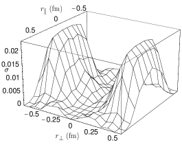
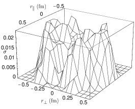
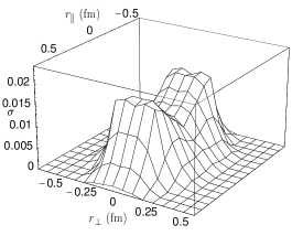
(a) (b) (c)

Figure 3: The $Z(2)$ action density for $2q2\bar{q}$ system at $\beta=2.5$. The size of the Wilson loops is $8\times 10$.

References

- [1] G. S. Bali, C. Schlichter and K. Schilling, Prog. Theor. Phys. Suppl. 131 (1998) 645.
- [2] V. Bornyakov et al., Nucl. Phys. Proc. Suppl. 106 (2002) 634.
- [3] Y. Koma, M. Koma, E. M. Ilgenfritz, T. Suzuki and M. I. Polikarpov, arXiv:hep-lat/0302006; F. V. Gubarev, E. M. Ilgenfritz, M. I. Polikarpov and T. Suzuki, Phys. Lett. B 468 (1999) 134.
- [4] L. Del Debbio, M. Faber, J. Greensite and S. Olejnik, Phys. Rev. D 55 (1997) 2298; M. Faber, J. Greensite and S. Olejnik, Phys. Rev. D 57 (1998) 2603.
- [5] V. G. Bornyakov, A. V. Kovalenko, M. I. Polikarpov and D. A. Sigaev, JETP Lett. 76 (2002) 647 [Pisma Zh. Eksp. Teor. Fiz. 76 (2002) 771].
- [6] J. Fingberg, U. M. Heller and F. Karsch, Nucl. Phys. B 392 (1993) 493.
- [7] G. S. Bali, V. Bornyakov, M. Muller-Preussker and K. Schilling, Phys. Rev. D 54 (1996) 2863; V. G. Bornyakov, D. A. Komarov, M. I. Polikarpov and A. I. Veselov, arXiv:hep-lat/0210047.
- [8] P. Pennanen, A. M. Green and C. Michael, Phys. Rev. D 59 (1999) 014504.