MPP-2003-76
The long range properties of the compact U(1) lattice gauge theory with the multi-level algorithm

Abstract

The 4D compact U(1) lattice gauge theory (LGT) in the confinement phase is studied with the multi-level algorithm. The static potential, force and flux-tube profile between two static charges are precisely measured from correlation functions involving the Polyakov loop. Universality of the coefficient of the $1/r$ correction to the static potential, known as the Lüscher term, and the transversal width of the flux-tube profile are investigated.

1 Introduction

If the confining gauge theory is related to an effective bosonic string theory, the long range behavior of the potential between static charges separated by distance $r$ is expected to have the form:

$$V(r)=\sigma r+\mu+\frac{\gamma}{r}+O(\frac{1}{r^{2}}).$$ (1)

Here $\sigma$ is the string tension and $\mu$ denotes a constant. The third term is known as the Lüscher term [1], where the coefficient, $\gamma=-\pi(d-2)/24$ with space-time dimension $d$, is considered to be universal. The effective bosonic string theory also predicts that the width of the field energy distribution of the flux tube diverges logarithmically as $r\to\infty$ [2]. Recent Monte-Carlo simulations of various LGTs support Eq. (1) with high accuracy: the confinement phase of $Z\!\!\!Z_{2}$ LGT [3], SU(2) LGT [4] and SU(3) LGT [5].

In this report we investigate the long range properties of compact U(1) LGT in the confinement phase. From the Polyakov loop correlation function (PLCF), we extract the potential and force to see whether this theory also supports the presence of the universal correction to the static potential. We then measure the profile of the flux tube induced by the PLCF, and see the behavior of its width as a function of $r$. However, due to its strong coupling nature, the Monte Carlo simulation of compact U(1) LTG is numerically difficult, when its long range properties are of interest. To obtain reliable signals, we apply here the multi-level algorithm proposed by Lüscher and Weisz originally for SU(3) LGT [6], which helps to reduce statistical errors exponentially.

2 Numerical procedures

We adopt the terminology of Ref. [6]. To measure the PLCF, $\langle P^{*}P(R)\rangle$, where $R=r/a$, we take second-level averages of the two-link correlators $\mathbb{T}(m;R;i)=U_{4}^{*}(m)U_{4}(m+R\;\hat{i})$ with $m=(m_{s},m_{t})$ as

$$\mathbb{T}^{(2)}(m_{s},\bar{m}_{t};R;i)=[\mathbb{T}(m;R;i)\mathbb{T}(m+\hat{4};R;i)],$$ (2)

which is achieved by updating link variables except for the spatial links at $\bar{m}_{t}=1,3,\ldots,N_{t}-1$. $N_{t}$ is the timelike extent of the lattice volume. $i=1,2,3$ denote directions between the two charges. We call this procedure the internal update. We repeat the internal update until reasonably stable values for $\mathbb{T}^{(2)}$ are obtained. Then the PLCF at a spatial site $m_{s}$ is constructed as

$$\!\!\!\!\!\!\!\!\!\!\!\!P^{*}P(m_{s};R;i)\!=\!{\rm Re}\;\mathbb{T}^{(2)}(m_{s},1;R;i)$$

$$\!\!\!\!\!\!\!\!\times\mathbb{T}^{(2)}(m_{s},3;R;i)\cdots\mathbb{T}^{(2)}(m_{s},N_{t}-1;R;i).$$ (3)

The average with respect to $m_{s}$ and $i$ provides $[P^{*}P(R)]_{i_{c}}$. The desired expectation value is the average of $[P^{*}P(R)]_{i_{c}}$ for $i_{c}=1,2,\ldots,N_{c}$. In the actual measurements, we have also applied the multi-hit technique to the timelike link variables for $R\geq 2$ before constructing $\mathbb{T}$. The static potential and the corresponding force are taken as (neglecting terms of $O(e^{-\Delta EN_{t}})$)

$$\!\!\!\!\!\!\!\!\!\!\!\!aV(R)=-\frac{1}{N_{t}}\ln\langle P^{*}P(R)\rangle\;,$$ (4)

$$\!\!\!\!\!\!\!\!\!\!\!\!a^{2}F(\bar{R})=aV(R)-aV(R-1)\;,$$ (5)

where $\bar{R}=R-1/2+O(a)$.

In order to measure the flux-tube profile, one needs to compute a correlation function of the type

$$\langle{\cal O}(n)\rangle_{j}=\frac{\langle P^{*}P{\cal O}(n)\rangle_{0}}{\langle P^{*}P\rangle_{0}}-\langle{\cal O}\rangle_{0}\;,$$ (6)

where ${\cal O}$ is a local operator, $\langle\cdots\rangle_{j}$ denotes an average in the vacuum with the PLCF, and $\langle\cdots\rangle_{0}$ an average in the vacuum without such a source. To measure $\langle P^{*}P{\cal O}\rangle_{0}$ on the mid-plane between two static charges, we parameterize the position of the local operator $n$ as $n=(n_{i}\!=\!m_{i}\!+\!R/2,\;n_{j}\!=\!m_{j}\!+\!x,\;n_{k}\!=\!m_{k}\!+\!y,\;n_{t}\!=\!m_{t})$ and take the average of the two-link-local-operator correlator

$$\!\!\!\!\!\!\!\!\!\!\!\!\mathbb{TO}^{(2)}(m_{s},\bar{m}_{t};n;R;i)=$$

$$\!\!\!\![\mathbb{T}(m;R;i)\mathbb{O}(m+\hat{4};n;R;i)]\;.$$ (7)

with $\mathbb{O}(m;n;R;i)=U_{4}^{*}(m)U_{4}(m+R\hat{i}){\cal O}(n)$ in addition to $\mathbb{T}^{(2)}$. Combining $\mathbb{TO}^{(2)}$ and $\mathbb{T}^{(2)}$, we obtain $\langle P^{*}P{\cal O}\rangle_{0}$.

As local operators, we have used ${\cal O}_{E}(n)=i\bar{\theta}_{\mu\nu}(n)$ for the electric field, and ${\cal O}_{k}(n)=2\pi ik_{\mu}(n)$ for the monopole current as defined in Ref. [7]. Note that the second term of Eq. (6) vanishes for these operators since $\mathcal{O}_{E}$ and $\mathcal{O}_{k}$ are parity odd.

3 Numerical results

We generate a sequence of independent gauge field configurations, by using the Wilson gauge action of compact U(1) LGT on a $16^{4}$ lattice at $\beta=$ 0.98, 0.99, 1.00, 1.005 and 1.01. For the first three $\beta$ values, the configuration has been generated after 500 thermalization sweeps, and they were separated by 100 sweeps, where one Monte Carlo update has been achieved by 1HB/3OR. For $\beta=$ 1.005 and 1.01 the thermalization sweeps have been taken 1000 and 3000, respectively, with 1HB/5OR Monte Carlo update.

For the static potential and force, we have used $N_{c}=$ 1050, 1250, 2050, 2400 and 3200 configurations, respectively. The internal updates have been taken as $N_{\rm iupd}=$10000, 8000, 5000, 3000 and 1000. These numbers are optimized to measure the PLCF up to $R$ = 6 with $<10$ % errors, where the PLCF themselves take values from $10^{-3}$ to $10^{-17}$. From the force, we have introduced a scale based on Sommer’s relation $r_{0}^{2}F(r_{0})=1.65$. Lattice spacings in units of $r_{0}$ are found to be $a/r_{0}=$ 0.470, 0.422, 0.353, 0.305 and 0.217, respectively.

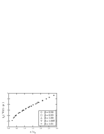
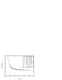
Figure 1: The static potential as a function of $r/r_{0}$. The constant $\mu$ is subtracted by using the fit result of Eq. (1), neglecting $O(1/r^{2})$ corrections.

Figure 2: The force as a function of $r/r_{0}$. The dotted line corresponds to the theoretical prediction of Eq. (1) up to $O(1/r^{2})$ corrections.

In Figs. 2 and 2, we show the static potential and force from all $\beta$ values. They show good scaling behaviors. We also plot the theoretical prediction for the force based on Eq. (1) in Fig. 2. We find that the long distance behavior is well-described by the function, $F=dV/dr=\sigma-\gamma/r^{2}$ with $\sigma r_{0}^{2}=1.65-\gamma=1.39$, which contains no fitting parameter. This supports the universality of $\gamma/r$ correction to the static potential. Surprisingly, another feature in common with non-Abelian gauge theories is that this function also fits the data down to relatively short distance to $r/r_{0}\sim 0.3$. For this, there is as yet no explanation.

We have measured flux-tube profiles with lengths $R=$ 3 to 6 at $\beta=$ 0.99 to 1.01 and $R=3$ to 5 at $\beta=0.98$. We have applied $N_{\mathrm{iupd}}=200\sim 8000$ depending on $R$ and $\beta$. The number of configurations are $N_{c}=300$ for all $\beta$ values. As an example, we show the profiles of the electric field and monopole current for $R=5$ at $\beta=0.98$ in Fig. 3, which is the longest flux tube in these measurements: $r/r_{0}=2.35$. Here we have taken the cylindrical average: $\rho=\sqrt{x^{2}+y^{2}}$ and $\varphi=\tan^{-1}(y/x)$. As shown in this figure, we have obtained very clean signals, however, rotational invariance for the monopole current profile seems not good due to the relatively large lattice spacing at $\beta=0.98$. For larger $\beta$, we obtained smoother curves.

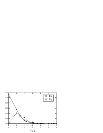
Figure 3: The profiles of the electric field ($E_{z}$) and monopole current ($k_{\varphi}$) for $R=5$ at $\beta=0.98$ as a function of the radius of the flux tube $\rho$.

There are several definitions of the width of the flux tube. Here, we have investigated this in terms of the peak radius of the monopole current profile, $\rho_{\rm eff}$. In order to find $\rho_{\rm eff}$ we have interpolated the on-axis data with a smooth curve. The result as a function of $r/r_{0}$ is shown in Fig. 4, where we have picked only the data with $R=5$ for all $\beta$ values; $\rho_{\rm eff}$ seems to grow as increasing $r$. However, we make no statement on the behavior whether the width diverges as $r\to\infty$. Also, since the rotational invariance is not good for small $\beta$ values, we have to check the validity of the smooth interpolation carefully. Further detailed analyses are in progress [8].

Figure 4: The peak radius of the monopole current profile as a function of $r/r_{0}$.

Acknowledgement

We are grateful to M. Lüscher and P. Weisz for useful discussions. The calculations were done on the SX-5 at the RCNP, Osaka University, Japan.

References

- [1] M. Lüscher, K. Symanzik and P. Weisz, Nucl. Phys. B173 (1980) 365.
- [2] M. Lüscher, G. Münster and P. Weisz, Nucl. Phys. B180 (1981) 1.
- [3] M. Caselle, M. Hasenbusch and M. Panero, JHEP 01 (2003) 057.
- [4] G.S. Bali, K. Schilling and C. Schlichter, Phys. Rev. D51 (1995) 5165; P. Majumdar, Nucl. Phys. B664 (2003) 213; S. Kratochvila and P. de Forcrand, hep-lat/0306011.
- [5] K.J. Juge, J. Kuti and C. Morningstar, Phys. Rev. Lett. 90 (2003) 161601; M. Lüscher and P. Weisz, JHEP 07 (2002) 049.
- [6] M. Lüscher and P. Weisz, JHEP 09 (2001) 010.
- [7] T.A. DeGrand and D. Toussaint, Phys. Rev. D22 (1980) 2478.
- [8] Y. Koma, M. Koma, and P. Majumdar, in preparation.