A numerical reinvestigation of the Aoki phase
with $N_{f}=2$ Wilson fermions at zero temperature

Abstract

We report on a numerical reinvestigation of the Aoki phase in lattice QCD with two flavors of Wilson fermions where the parity-flavor symmetry is spontaneously broken. For this purpose an explicitly symmetry-breaking source term $h\bar{\psi}i\gamma_{5}\tau^{3}\psi$ was added to the fermion action. The order parameter $\langle\bar{\psi}i\gamma_{5}\tau^{3}\psi\rangle$ was computed with the hybrid Monte Carlo algorithm at several values of $(\beta,\kappa,h)$ on lattices of sizes $4^{4}$ to $12^{4}$ and extrapolated to $h=0$. The existence of a parity-flavor breaking phase can be confirmed at $\beta=4.0$ and $4.3,$ while we do not find parity-flavor breaking at $\beta=4.6$ and $5.0$.

I Introduction

Spontaneous breaking of chiral symmetry is one of the main non-perturbative phenomena of QCD explaining many features of the hadronic world, in particular of hadrons containing $u$, $d$ and/or $s$ quarks. QCD allows us to interpret the light octet mesons as Goldstone bosons. The four-dimensional (Euclidean) lattice discretization of QCD provides a unique ab initio non-perturbative approach. However, in this approach chiral symmetry has to be treated with special care. At present, on the lattice this symmetry is best realized by satisfying the Ginsparg-Wilson relation GinWil for the lattice Dirac operator, e.g. ​​, employing the so-called overlap operator NarNeu ; Neu , or using the five-dimensional domain wall fermion ansatz KapSham ; Sham ; FurSham . In both cases the Wilson-Dirac operator $W(m_{0})$ (with a bare mass parameter $m_{0}\in(-2,0)$) serves as an input for the fermionic part of the lattice discretized action.

For the Wilson-Dirac operator (which breaks chiral invariance explicitly) Aoki Aoki_first has argued that in a certain range of the hopping parameter $\kappa$ (or the bare mass $m_{0}$) there is a phase in which parity-flavor symmetry is spontaneously broken, in the sense that a condensate as defined in Eq. (1) exists and is non-vanishing. In agreement with the literature we call it the Aoki phase. When $\kappa$ approaches the border lines of this phase all pion masses tend to zero because one is approaching a second order phase transition. In the whole Aoki phase the charged pion states are expected to remain massless (in the case of $N_{f}=2$ flavors) since they appear to be the Goldstone bosons related to parity-flavor breaking, whereas the neutral pion should become massive again. The general phase structure as proposed by Aoki is shown in Fig. 1. Some numerical results supporting this picture were presented in Refs. Aoki_first ; Aoki_next ; AokGoc1 ; AokGoc2 ; AokKanUka ; BitLATT97 .

It has been questioned whether the Aoki phase survives the continuum limit (in the sense of extending to $\beta=\infty$) or, alternatively, ends somewhere at finite $\beta$, perhaps before the scaling regime is reached. Previous investigations of this problem did not yield a unique answer AokGoc2 ; AokKanUka ; BitLATT97 ; ShaSin ; BitPRD ; Aoki_summary . In this paper we present results of a more thorough numerical analysis of this question. As has been discussed recently GolSham , the answer is of relevance for the locality behavior and the restoration of chiral invariance in quenched and full QCD with Ginsparg-Wilson and domain wall fermions. Accordingly, the region of the Aoki phase has to be avoided in such computations in order not to spoil physical reliability.

Our investigation was carried out for full lattice QCD with $N_{f}=2$ flavors of unimproved Wilson fermions using the standard plaquette gauge action. It includes a careful extrapolation of $\langle\bar{\psi}i\gamma_{5}\tau^{3}\psi\rangle$ to vanishing external field. It shows that the Aoki phase is unlikely to extend beyond $\beta=4.6$ (which confirms early conclusions in Ref. BitPRD ).

The outline of our paper is as follows. In Sec. II we discuss the proposed phase structure in greater detail. Section III provides details of our numerical simulations. In Sec. IV we present our numerical results. Section V contains the discussion and our conclusions.

II The proposed phase structure

Aoki, in his last status report Aoki_summary , has discussed the lattice results supporting the view that for lattice QCD with $N_{f}=2$ Wilson fermions there exists a parity-flavor breaking phase which is separated from an unbroken phase (or from unbroken phases) by second order phase transition lines. The conjectured phase structure in the $(g^{2},m_{0})$ plane is shown on the left-hand side of Fig. 1. As can be seen from this figure, two of these critical lines run from strong coupling to the weak coupling limit, while further critical lines are confined to the weak coupling region. At zero coupling, pairs of these transition lines join at points referring to the different fermion doublers.

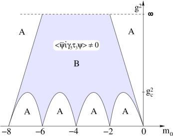
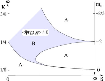
Figure 1: The phase diagram proposed by Aoki et al. in the $(g^{2},m_{0})$ plane (left-hand side) and in the $(\beta,\kappa)$ plane (right-hand side). The shaded region labeled $B$ denotes the phase where flavor and parity are spontaneously broken. Both symmetries are conserved in regions labeled $A$.

Aoki Aoki_next has further claimed that along the critical lines the pion triplet is massless. The neutral pion becomes massless only on the critical lines, due to the presence of a second order phase transition, while the charged pions turn massless on the critical lines and remain massless inside the Aoki phase signaling that flavor symmetry is broken.

When simulating the theory it is natural to draw the phase diagram in the $(\beta,\kappa)$ plane . Using the well known relations $\kappa=1/(2m_{0}+8)$ and $\beta=6/g^{2}$, the proposed phase structure is mapped to this plane as shown on the right-hand side of Fig. 1. Therein the symmetry $m_{0}\leftrightarrow-(m_{0}+8)$ is hidden in the reflection $\kappa\leftrightarrow-\kappa$ which is not made explicit for simplicity. The critical line $\kappa_{c}(\beta)$ which runs from $\beta=0$ to infinity is nothing but the chiral limit line of lattice QCD. Thus the scenario proposed by Aoki et al. might explain why all pions are massless along this line despite the fact that Wilson fermions explicitly break chiral symmetry.

In principle, the Aoki phase could be expected to exist for all values of $\beta$. In the strong coupling region the existence of such a phase was verified by performing numerical simulations of QCD with Wilson fermions as summarized in Aoki_summary and reconsidered in BitLATT97 . For this purpose a so-called twisted mass term $h\bar{\psi}i\gamma_{5}\tau^{3}\psi$ was added to the action which explicitly breaks parity-flavor symmetry. Without an external field $h$ coupling to $\bar{\psi}i\gamma_{5}\tau^{3}\psi$, the parameter $\langle\bar{\psi}i\gamma_{5}\tau^{3}\psi\rangle$ would always be zero on a finite lattice. $\langle\bar{\psi}i\gamma_{5}\tau^{3}\psi\rangle$ has to be measured for varying lattice size $V$ and non-vanishing $h$ values. The order parameter $\langle\bar{\psi}i\gamma_{5}\tau^{3}\psi\rangle_{h=0}$ is then obtained by taking the double limit in the following order

$$\langle\bar{\psi}i\gamma_{5}\tau^{3}\psi\rangle_{h=0}=\lim_{h\rightarrow 0}\lim_{V\rightarrow\infty}\langle\bar{\psi}i\gamma_{5}\tau^{3}\psi\rangle\,.$$ (1)

In the literature one finds numerical results from quenched AokKanUka and unquenched AokGoc2 ; BitLATT97 simulations at finite $h$ which support the existence of a parity-flavor breaking phase, at least for $\beta\leq 4.0$. However, extrapolations in order to carry out the double limit (1) had not been performed.

Going to larger values of $\beta$ there are contradictory statements about the existence of such a broken phase. Bitar BitPRD has come to the conclusion that there is no Aoki phase for $\beta\geq 5.0$. However, results from quenched simulations AokKanUka suggest that the finger structure anticipated by Aoki exists.

Aoki’s scenario was also challenged in Refs. BitHelNar ; EdwHelNarSin ; EdwHelNar . In particular, in Ref. BitHelNar it has been argued that flavor and parity are not violated at finite lattice spacing. The authors have rather proposed that the Aoki phase has to be interpreted as a phase with massless quarks and spontaneous chiral symmetry breaking.

In Ref. ShaSin the controversy has been concisely elucidated in the sense that, at finite lattice spacing $a$, the Wilson lattice theory is able to exhibit flavor and parity breaking under certain circumstances. The authors have also demonstrated that the results of EdwHelNarSin ; EdwHelNar concerning the spectrum of the Hermitean Wilson-Dirac operator $\gamma_{5}W(m_{0})$ (actually obtained for quenched or partially quenched lattice QCD) lend support, if correctly interpreted, to a non-vanishing condensate as defined in Eq. (1).

In terms of an effective chiral Lagrangian, it has been pointed out in Ref. ShaSin that only two possible scenarios may exist, depending on the sign of one coupling coefficient. In the first case, the Aoki picture Aoki_next is exactly reproduced, whereas in the second case all pion masses remain degenerate and non-vanishing over the whole $(g^{2},m_{0})$ plane such that no Aoki phase exists at all. If the first case applies to lattice QCD all the way to the continuum limit specific predictions concerning the $a$ dependence of the neutral pion mass and of the width of the Aoki finger pointing towards $(m_{0}=0,g^{2}=0)$ have been made. However, if the sign turns to the second case the Aoki phase ceases to exist at strong coupling and those predictions do not apply.

After that, the only remaining question is whether the Aoki phase really persists until the continuum limit and, if it does so, how it shrinks to the point $(m_{0}=0,g^{2}=0)$. Only numerical simulations can clarify whether there is a strip of parity-flavor breaking phase in lattice QCD with Wilson fermions extending to infinite $\beta$.

Figure 2: Results for $\langle\bar{\psi}i\gamma_{5}\tau^{3}\psi\rangle$ as a function of $\kappa$ and $h$ at $\beta=4.0$ on a $6^{4}$ lattice.

III Simulation details

We have simulated lattice QCD with two flavors of (unimproved) Wilson fermions with (the $\Phi$ version of) the hybrid Monte Carlo algorithm Duane ; Gottlieb where an even/odd decomposition even-odd has been employed. An explicitly symmetry breaking source term was added to the Wilson fermion matrix $M_{W}$, i.e. the two-flavor fermion matrix was given by

$$M(h)=M_{W}+hi\gamma_{5}\tau^{3}.$$ (2)

The simulations were performed on lattices ranging from $4^{4}$ to $12^{4}$ at $\beta$ values 4.0, 4.3, 4.6, and 5.0, with $\kappa$ and $h$ in the intervals $0.15\leq\kappa\leq 0.28$ and $0.003\leq h\leq 0.04$, respectively.

In our study we measured $\langle\bar{\psi}i\gamma_{5}\tau^{3}\psi\rangle$ as a function of $\kappa$ at finite $h$. The parameter $\langle\bar{\psi}i\gamma_{5}\tau^{3}\psi\rangle$, which is proportional to the imaginary part of the trace of $\gamma_{5}M^{-1}(h)$, was averaged over 100–1000 gauge field configurations (see Table 2) separated by trajectories of length 1. The trace was measured with a stochastic estimator Horsley .

For illustration, results for $\langle\bar{\psi}i\gamma_{5}\tau^{3}\psi\rangle$ from a $6^{4}$ lattice at $\beta=4.0$ are shown in Fig. 2. The location of the peak determines the region where subsequent simulations on larger lattices and smaller $h$ were performed. In Fig. 2 the peak is around $\kappa=0.22$. It becomes sharper as $h$ decreases. We have increased the lattices until measurements agreed within errors such that we can treat our largest lattices as infinitely large. The extrapolation to vanishing $h$ is described in the following section.

IV Extrapolating to vanishing external field

In Fig. 3 an analysis of $\langle\bar{\psi}i\gamma_{5}\tau^{3}\psi\rangle$ data is shown for $\beta=4.0$ and $4.3$. As can be seen from the upper and lower left plot the interesting region is around $\kappa=0.22$ and $\kappa=0.21,$ respectively. At these $(\beta,\kappa)$ pairs further simulations were performed in order to control finite-size effects. Data from these simulations are shown in the center plots of Fig. 3. No finite size effects are visible in the plots except for data from the $4^{4}$ lattice at $\beta=4.0$. Hence, the measurements of $\langle\bar{\psi}i\gamma_{5}\tau^{3}\psi\rangle$ from the largest lattice at each $h$ can be considered to lie within errors on the infinite volume envelope.

The question arises how to fit these data properly. Motivated from the mean field equation

$$h=A_{0}\sigma^{3}+A_{1}\!\cdot\!\left(\kappa-\kappa_{c}\right)\sigma\qquad\textrm{with}\quad\sigma\equiv\langle\bar{\psi}i\gamma_{5}\tau^{3}\psi\rangle$$ (3)

we use the ansatz

$$\sigma(h)=A+Bh^{C}+\ldots\quad.$$ (4)

It is instructive to look at so-called Fisher plots Fisher ; Hinnerk2 (see the right-hand side of Fig. 3). From Eq. (3) one expects data for $\kappa\leq\kappa_{c}$ to lie on straight lines ending at the origin or at the abscissa, while within the broken phase they should lie on straight lines ending at the ordinate. As can be seen from the Fisher plots obtained the data do not lie on straight lines and therefore do not behave mean-field like.

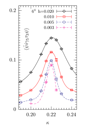
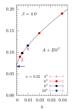
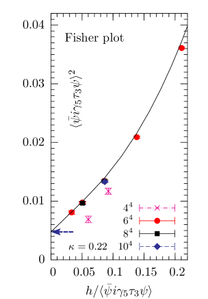
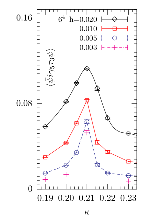
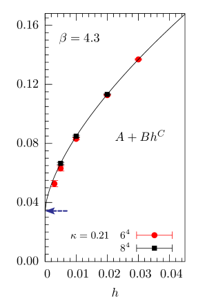
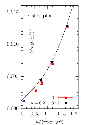
Figure 3: In the left column data for $\langle\bar{\psi}i\gamma_{5}\tau^{3}\psi\rangle$ from a $6^{4}$ lattice are shown as a function of $\kappa$ at several values of $h$ (the lines are spline interpolations to guide the eye). The extrapolation to $h=0$ in the infinite volume limit is shown in the center column of this figure. The right column shows the Fisher plots with the corresponding fitting function. The upper row shows results for $\beta=4.0$, the lower one for $\beta=4.3$.

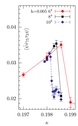
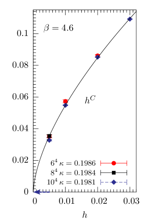
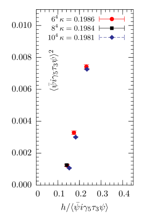
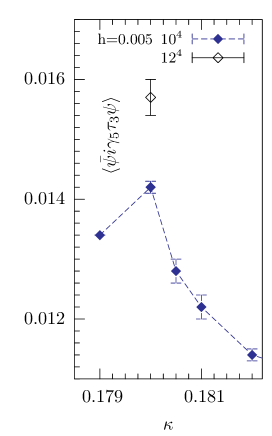
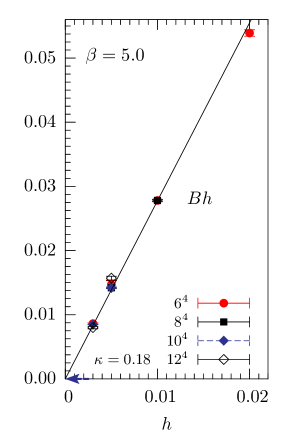
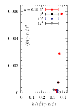
Figure 4: In the left column data for $\langle\bar{\psi}i\gamma_{5}\tau^{3}\psi\rangle$ from lattices of various sizes are shown as a function of $\kappa$ at $h=0.005$ fixed (the lines are drawn to guide the eye). The extrapolation to $h=0$ in the infinite volume limit is shown in the center column. In the right column the corresponding Fisher plots are shown. The upper row contains data at $\beta=4.6$ from lattices of sizes $6^{4}$, $8^{4}$ and $10^{4}$. The lower row shows measurements for $\beta=5.0$ from lattices of size from $6^{4}$ to $12^{4}$.

Using Eq. (4) with the mean field value $C=1/3$ results in unstable fitting functions, but taking $C$ as a free parameter instead, the ansatz describes the data well. In fact, the parameter of interest $A$ is robust against the introduction of linear and quadratic correction terms (see Table 1). Furthermore, the fit parameters $B$ and $C$ agree within errors for both values of $\beta$, even when introducing corrections. We conclude that the order parameter $\langle\bar{\psi}i\gamma_{5}\tau^{3}\psi\rangle_{h=0}$ is non-zero at $(\beta,\kappa)=(4.0,0.22)$ and $(4.3,0.21)$.

Measurements for $\langle\bar{\psi}i\gamma_{5}\tau^{3}\psi\rangle$ at $\beta=4.6$ are shown in the upper row of Fig. 4. Looking at the upper left plot of the figure one sees that $\langle\bar{\psi}i\gamma_{5}\tau^{3}\psi\rangle$ still has a peak at finite $h$. The peak becomes narrower and its position is shifted from $\kappa=0.1986$ to $\kappa=0.1981$ as the lattice size is increased from $6^{4}$ to $10^{4}$. Taking the results from the $10^{4}$ lattice at $\kappa=0.1981$, a fit using Eq. (4) can be performed. However, due to low statistics the point at $h=0.005$ was discarded and therefore some fit parameters had to be fixed. Using the fit results from the two lower values of $\beta$, the parameter $A$, $B$ and $C$ were alternately fixed to reasonable values. The extrapolation is consistent with a vanishing order parameter (see Table 1). The same result is obtained by inspection of the Fisher plot in Fig. 4 where the data seem to lie on a line ending on the abscissa. This means that the order parameter $\langle\bar{\psi}i\gamma_{5}\tau^{3}\psi\rangle_{h=0}$ vanishes at $\beta=4.6$.

In addition, the parameters $B$ and $C$ agree within errors for all three values of $\beta$ as can be seen from Table 1. Therefore, we also fitted the data globally using ansatz (4) where $B$ and $C$ are common to all data, while the parameters $A_{\beta}$ and $D_{\beta}$ are different for each $\beta$. In Table 3 the fit results are shown. In agreement with the results presented above, the order parameter $\langle\bar{\psi}i\gamma_{5}\tau^{3}\psi\rangle_{h=0}$ is found to be finite at $\beta=4.0$ and $\beta=4.3$, while it vanishes at $\beta=4.6$. Furthermore, their values are robust against the introduction of a correction term linear in $h$, while $B$ and $C$ are sensitive.

At $\beta=5.0$ a vanishing order parameter becomes manifest. As can be seen from the lower row of Fig. 4 there is still a peak. However, the extrapolation of $\langle\bar{\psi}i\gamma_{5}\tau^{3}\psi\rangle$ to $h=0$ at $\kappa=0.18$ as well as the Fisher plot do not support a finite value of $\langle\bar{\psi}i\gamma_{5}\tau^{3}\psi\rangle_{h=0}$ at $\beta=5.0$.

fit	A	B	C	D	E	$\chi^{2}/\textsc{ndf}$
	$\beta=4.0$  $\kappa=0.22$
1	0.068(4)	1.07(9)	0.67(3)	0	0	0.80
2a	0.067(3)	1	0.66(2)	0.1(1)	0	0.83
2b	0.067(3)	1.03(11)	$2/3$	0.1(3)	0	0.81
3a	0.066(3)	1	0.65(1)	0	1(1)	0.98
3b	0.067(2)	1.05(4)	$2/3$	0	0.1(17)	0.84
	$\beta=4.3$  $\kappa=0.21$
1	0.034(1)	0.99(3)	0.65(1)	0	0	0.08
2a	0.034(1)	1	0.65(1)	-0.02(4)	0	0.08
2b	0.035(1)	1.11(4)	$2/3$	-0.2(1)	0	0.09
3a	0.035(1)	1	0.65(1)	0	-0.2(6)	0.08
3b	0.036(1)	1.06(1)	$2/3$	0	-1.2(9)	0.13
	$\beta=4.6$  $\kappa=0.1981$
1a	0	1	0.63(1)	0	0	3.21
1b	0.001(2)	1	0.63(6)	0	0	4.82
1c	0	0.97(3)	0.62(9)	0	0	3.62
2a	0	1	0.63(1)	-0.05(5)	0	3.36
2b	0.0005(8)	1	0.63	-0.03(3)	0	3.87
3a	0	1	0.63(1)	0	-1(1)	2.41
3b	0.0003(4)	1	0.63	0	-0.9(7)	2.79

Table 1: The parameters of the ansatz $\sigma(h)=A+Bh^{C}+Dh+Eh^{2}$ fitted to the data for $\langle\bar{\psi}i\gamma_{5}\tau^{3}\psi\rangle$ at $\beta=4.0$, $4.3$ and $4.6$ with no, linear or quadratic corrections (labeled as 1, 2 or 3). At each $h$ the result from the largest lattice was used in the fit (for details see Table 2). The data at $h=0.003$ were discarded because these are from a $6^{4}$ lattice. Also the result at $\beta=4.6$ and $h=0.005$ was not taken into account due to low statistics. Fixed parameters are presented by their value without giving an error. In each case the first fit (bold numbers) was used in Figs. 3 and 4, respectively.

		$h$
$\beta$	$\kappa$	$0.005$		$0.01$		$0.02$		$0.03$		$0.04$
4.0	0.2200	$8^{4}$	250	$10^{4}$	146	$6^{4}$	1000	–	–	$6^{4}$	1000
4.3	0.2100	$8^{4}$	300	$8^{4}$	500	$8^{4}$	250	$6^{4}$	500	–	–
4.6	0.1981	–	–	$10^{4}$	170	$10^{4}$	250	$10^{4}$	200	–	–

Table 2: Statistics used for the final analysis (extrapolation) at selected $\kappa$ values for $\beta=4.0$, $4.3$ and $4.6$. For the respective values of $h$ given in the first row in the second column we report the number of trajectories produced for each lattice size. A similar statistic was used for scanning at neighboring $\kappa$ values.

fit	$\beta$	Aβ	B	C	Dβ	$\chi^{2}/\textsc{ndf}$
	4.0	0.063(2)			0
1	4.3	0.032(2)	1.0(1)	0.64(2)	0	3.4
	4.6	0.004(2)			0
	4.0	0.065(2)			-0.8(3)
2	4.3	0.034(2)	1.5(2)	0.71(2)	-0.8(3)	2.4
	4.6	0.004(2)			-0.7(3)

Table 3: The parameters of the ansatz $\sigma(h)=A_{\beta}+Bh^{C}+D_{\beta}h$   fitted to the data in Table 2 for $\langle\bar{\psi}i\gamma_{5}\tau^{3}\psi\rangle$ at $\beta=4.0$, $4.3$ and $4.6$ with no (fit 1) and linear (fit 2) corrections. The parameter $B$ and $C$ are common to all data, while for each $\beta$ there is a separate value for $A_{\beta}$ and $D_{\beta}$, respectively. Fixed parameters are presented by their value without giving an error.

V Discussion

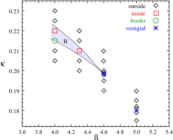
Figure 5: The part of the phase diagram studied in this work. Squares denote ($\beta,\kappa$) pairs where a finite value of $\langle\bar{\psi}i\gamma_{5}\tau^{3}\psi\rangle_{h=0}$ is found. Diamonds refer to points where $\langle\bar{\psi}i\gamma_{5}\tau^{3}\psi\rangle_{h=0}=0$. Stars denote points where a finite value of $\langle\bar{\psi}i\gamma_{5}\tau^{3}\psi\rangle_{h=0}$ is uncertain. The lines indicate the position of the critical lines $\kappa^{(l)}_{c}(\beta)$ and $\kappa^{(u)}_{c}(\beta)$. The shaded region labeled $B$ refers to the parity-flavor breaking phase. The point ($\beta,\kappa$)=($4.0,0.215$) marked by a circle seems to lie very close to the border of the broken phase.

In this study we have investigated how far a parity-flavor breaking phase in lattice QCD with two flavors of dynamical Wilson fermions at zero temperature extends in $\beta$. An explicitly symmetry breaking term, the twisted mass term $h\bar{\psi}i\gamma_{5}\tau^{3}\psi$, was added to the Wilson fermion matrix. The phase diagram was explored in the rectangle $4.0\leq\beta\leq 5.0$ and $0.15\leq\kappa\leq 0.28$.

We have presented hybrid Monte Carlo results for the order parameter $\langle\bar{\psi}i\gamma_{5}\tau^{3}\psi\rangle$. The existence of a parity-flavor breaking phase could be confirmed at $(\beta,\kappa)=(4.0,0.22)$ and $(4.3,0.21)$, where $\langle\bar{\psi}i\gamma_{5}\tau^{3}\psi\rangle$, measured at finite $h$, extrapolates to a finite value at $h=0$ in the infinite volume limit. No parity-flavor breaking was found at $\beta=4.6$ and $\beta=5.0$. This suggests a phase structure as shown in Fig. 5. Two squares in Fig. 5 mark points where we were able to confirm the Aoki phase. Two stars mark points where $\langle\bar{\psi}i\gamma_{5}\tau^{3}\psi\rangle$ has a peak at finite $h$, but where our extrapolation to $h=0$ is consistent with a vanishing order parameter. Consequently these stars are labeled vestigial.

According to these results, the Aoki phase for $T=0$ seems to end close to $\beta=4.6$ and $\kappa=0.1981$. Rough estimates for the upper $\kappa^{(u)}_{c}$ and lower $\kappa^{(l)}_{c}$ bound of the Aoki phase are

$$\beta=4.0: \;0.215\simeq\kappa^{(l)}_{c}<0.220\quad 0.220<\kappa^{(u)}_{c}<0.225$$

$$\beta=4.3: \;0.205<\kappa^{(l)}_{c}<0.210\quad 0.210<\kappa^{(u)}_{c}<0.215\,.$$

The pair $(\beta,\kappa)=(4.0,0.215)$ seems to be quite close to the lower boundary. We conclude this from the behavior of $\langle\bar{\psi}i\gamma_{5}\tau^{3}\psi\rangle$ in conjunction with the behavior of the pion norm BKR (which also has been measured during our simulations). At this $(\beta,\kappa)$ pair $\langle\bar{\psi}i\gamma_{5}\tau^{3}\psi\rangle$ extrapolates to zero at $h=0$, whereas the pion norm seems to diverge as $h\rightarrow 0$. Such behavior is expected close to critical lines $\kappa_{c}(\beta)$.

Referring to the discussion of the anticipated phase diagram in Sec. II, the results presented here do not indicate a parity-flavor breaking phase at $\beta\geq 4.6$ which was originally claimed to exist at all $\beta$ (see Fig. 1). This is suggested not only by the extrapolation of $\langle\bar{\psi}i\gamma_{5}\tau^{3}\psi\rangle$ to $h=0$ in Sec. IV, which yields $\langle\bar{\psi}i\gamma_{5}\tau^{3}\psi\rangle_{h=0}=0$ at $\beta=4.6$ and $\beta=5.0$, but also by the observation that the peak of $\langle\bar{\psi}i\gamma_{5}\tau^{3}\psi\rangle$ decreases in height and width as $\beta$ increases. The parity-flavor breaking phase seems to be pinched off near $\beta=4.6$ as illustrated in Fig. 5. From the numerical point of view we agree with Bitar BitPRD , who has found no evidence of such a broken phase for $\beta\geq 5.0$.

On the other hand, although $\langle\bar{\psi}i\gamma_{5}\tau^{3}\psi\rangle$ decreases, a non-vanishing value at $h=0$ in the infinite volume limit is not excluded. A decreasing width could have been expected from the phase structure in Fig. 1. The fact that the peak becomes narrower implies that a high resolution scan in $\kappa$ is required at larger values of $\beta$. In addition, lattices much larger than $12^{4}$ would be needed (which is beyond our presently available computing resources). With this in mind it is comprehensible that the results presented in Ref. BitPRD could not indicate a broken phase for $\beta\geq 5.0$ just because of the small lattice sizes used ($6^{4}$, $8^{4}$ and $10^{4}$). While we find no numerical evidence for the existence of the Aoki phase for $\beta\geq 4.6$ one cannot exclude that the phase might be found with methods to be invented similar to reweighting.

A further interesting observation we made is that the data behave differently when approaching the parity-flavor breaking phase at fixed $\beta$ from $\kappa>\kappa^{(u)}_{c}$ compared with the approach from $\kappa<\kappa^{(l)}_{c}$. First, the peaks of $\langle\bar{\psi}i\gamma_{5}\tau^{3}\psi\rangle$ as a function of $\kappa$ are asymmetric. Second, an autocorrelation analysis of $\langle\bar{\psi}i\gamma_{5}\tau^{3}\psi\rangle$ shows that measurements to the right of the peak (above of the Aoki phase) are significantly stronger correlated than at all smaller $\kappa$ values.

In light of the possible scenarios discussed by Sharpe and Singleton ShaSin it might be worthwhile to invest more computing power in a study of both the width of the Aoki finger and the detailed behavior of the neutral pion mass inside and outside the Aoki phase with respect to the lattice spacing dependence. For the case of $N_{f}=2$ dynamical (unimproved) Wilson fermions with standard Wilson gauge action, however, the impossibility of matching the $\pi$ and $\rho$ masses in the interval $3.5<\beta<5.3$ is known BitEdwHelKen , which means that scaling is strongly violated. Thus the result of the present paper, confining the Aoki phase to $\beta<4.6$, unfortunately does not allow this potentially interesting comparison with chiral perturbation theory.

In view of the fact that the region above the Aoki phase ($\kappa>\kappa^{(u)}_{c}$) is the region of interest for the insertion of the Wilson-Dirac operator into the overlap form Neu of the massless fermion operator an even more extensive investigation of this area might be worthwhile to do.

References

- (1) P. H. Ginsparg and K. G. Wilson, Phys. Rev. D 25, 2649 (1982).
- (2) R. Narayanan and H. Neuberger, Phys. Rev. Lett. 71, 3251 (1993); Nucl. Phys. B 412, 574 (1994); Nucl. Phys. B 443, 305 (1995).
- (3) H. Neuberger, Phys. Lett. B 417, 141 (1998); Phys. Lett. B 427, 353 (1998).
- (4) D. V. Kaplan, Phys. Lett. B 288, 342 (1992).
- (5) Y. Shamir, Nucl. Phys. B 406, 90 (1993).
- (6) V. Furman and Y. Shamir, Nucl. Phys. B 439, 54 (1995).
- (7) S. Aoki, Phys. Rev. D 30, 2653 (1984).
- (8) S. Aoki, Phys. Rev. Lett. 57, 3136 (1986).
- (9) S. Aoki and A. Gocksch, Phys. Lett. B 231, 449 (1989); Phys. Lett. B 243, 409 (1990).
- (10) S. Aoki and A. Gocksch, Phys. Rev. D 45, 3845 (1992).
- (11) S. Aoki, T. Kaneda, and A. Ukawa, Phys. Rev. D 56, 1808 (1997).
- (12) K. M. Bitar, Nucl. Phys. Proc. Suppl. 63, 829 (1998).
- (13) S. Sharpe and R. Singleton, Jr., Phys. Rev. D 58, 074501 (1998).
- (14) K. M. Bitar, Phys. Rev. D 56, 2736 (1997).
- (15) S. Aoki, Nucl. Phys. Proc. Suppl. 60A, 206 (1998), and references given therein.
- (16) M. Golterman and Y. Shamir, Phys. Rev. D 68, 074501 (2003).
- (17) K. M. Bitar, U. M. Heller, and R. Narayanan, Phys. Lett. B 418, 167 (1998).
- (18) R. G. Edwards, U. M. Heller, R. Narayanan, and R. Singleton, Jr., Nucl. Phys. B 518, 319 (1998).
- (19) R. G. Edwards, U. M. Heller, and R. Narayanan, Nucl. Phys. B 535, 403 (1998).
- (20) S. Duane, A. D. Kennedy, B. J. Pendleton, and D. Roweth, Phys. Lett. B 195, 216 (1987).
- (21) S. Gottlieb, W. Liu, D. Toussaint, R. L. Renken, and R. L. Sugar, Phys. Rev. D 35, 2531 (1987).
- (22) R. Gupta et al., Phys. Rev. D 40, 2072 (1989).
- (23) K. Bitar, A. D. Kennedy, R. Horsley, S. Meyer, and P. Rossi, Nucl. Phys. B 313, 348 (1989).
- (24) J. S. Kouvel and M. E. Fisher, Phys. Rev. 136, A1626 (1964).
- (25) M. Göckeler et al., Nucl. Phys. B 487, 313 (1997).
- (26) K. Bitar, A. D. Kennedy, and P. Rossi, Phys. Lett. B 234, 333 (1990).
- (27) K. M. Bitar, R. G. Edwards, U. M. Heller, and A. D. Kennedy, Phys. Rev. D 54, 3546 (1996).