The ATLAS discovery potential for a heavy charged Higgs boson in $gg\to tbH^{\pm}$ with $H^{\pm}\to tb$

Abstract

The feasibility of detecting a heavy charged Higgs boson, $\mbox{$m_{\mathrm{H}^{\pm}}$}>\mbox{$m_{\mathrm{t}}$}+m_{b}$, decaying in the $\mbox{$\mathrm{H}^{\pm}$}\rightarrow tb$ channel is studied with the fast simulation of the atlas detector. We study the $gg\rightarrow{\mbox{$\mathrm{H}^{\pm}$}}tb$ production process at the lhc which together with the aforementioned decay channel leads to four $b$–quarks in the final state. The whole production and decay chain reads $gg\rightarrow tb\mbox{$\mathrm{H}^{\pm}$}\rightarrow t\bar{t}b\bar{b}\rightarrow b\bar{b}b\bar{b}l\nu\bar{q}q^{\prime}$. Combinatorial background is a major difficulty in this multi–jet environment but can be overcome by employing multivariate techniques in the event reconstruction. Requiring four $b$–tagged jets in the event helps to effectively suppress the Standard Model backgrounds but leads to no significant improvement in the discovery potential compared to analyses requiring only three $b$–tagged jets. This study indicates that charged Higgs bosons can be discovered at the lhc up to high masses ($\mbox{$m_{\mathrm{H}^{\pm}}$}>400\,\mbox{$\mathrm{GeV}$}$) in the case of large $\tan\!\beta$.

I Introduction

The only particle predicted by the Standard Model (SM) that has so far not been detected is the Higgs boson. In the Minimal Supersymmetric extension to the Standard Model (MSSM) Nilles:1984ge ; Haber:1985rc the Higgs sector is enlarged to contain 5 particles: 3 neutral ($\mathrm{h}^{0}$,$\mathrm{H}^{0}$,$\mathrm{A}^{0}$) and two charged ($\mathrm{H}^{+}$,$\mathrm{H}^{-}$) Higgs bosons. Whereas the detection of one neutral Higgs bosons would be compatible with both the SM and the MSSM, the detection of a charged spin–0 particle such as the charged Higgs boson predicted by the MSSM would unequivocally point towards new physics beyond the SM. This note describes the potential of the atlas experiment to detect a heavy charged Higgs boson, i.e. a charged Higgs boson heavier than the top quark, decaying in the $\mbox{$\mathrm{H}^{\pm}$}\rightarrow tb$ channel.

Other experiments have also searched for the charged Higgs boson and set lower limits on the charged Higgs boson mass. The combined LEP experiments provide a preliminary exclusion of charged Higgs bosons with $\mbox{$m_{\mathrm{H}^{\pm}}$}<78.6\,\mbox{$\mathrm{GeV}$}$ at the $95\,\%$ CL unknown:2001xy . At the Tevatron, CDF and D0 searched for the charged Higgs boson in the decay of top quarks produced in $p\bar{p}\rightarrow t\bar{t}$ reactions. These searches exclude the low and high $\tan\!\beta$ regions up to charged Higgs masses of $\approx 160\,\mbox{$\mathrm{GeV}$}$ Affolder:1999au ; Abazov:2001md .

The Higgs sector of the MSSM is determined by two free parameters at tree level, most often chosen to be the mass of the CP–odd neutral Higgs boson, $m_{\mathrm{A}}$, and the ratio of the vacuum expectation values of the two electroweak Higgs doublets, parametrised by $\tan\!\beta$. The decay modes of the charged Higgs boson in the MSSM are given as a function of the charged Higgs mass in Figure 1 for two different values of $\tan\!\beta$, $1.5$ and $30$.

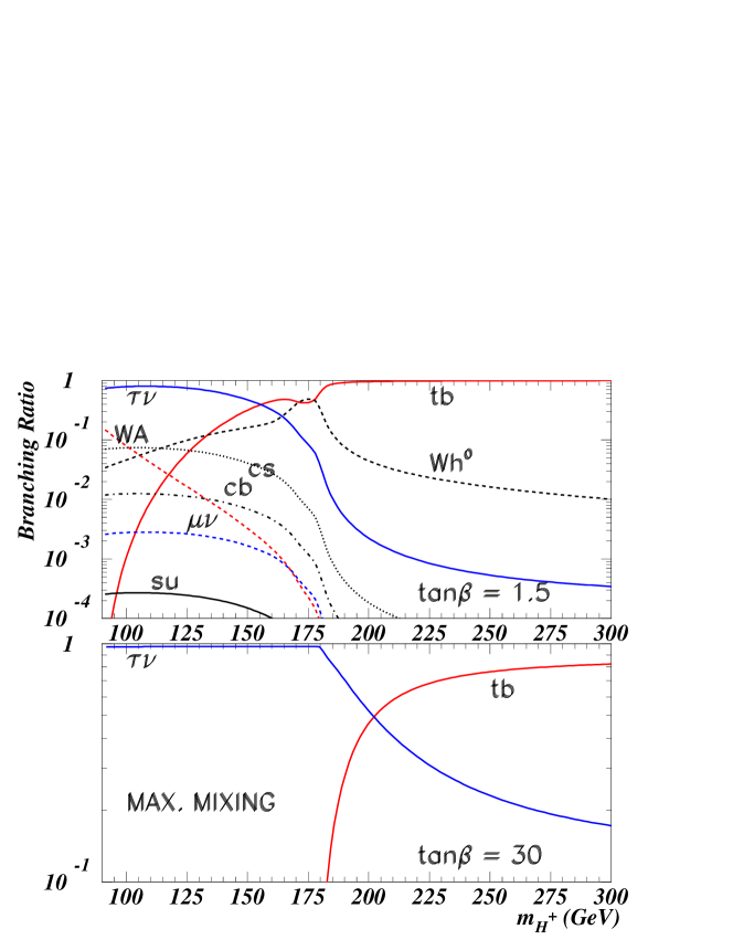
Figure 1: Branching ratios for different decay channels of the charged Higgs boson in the MSSM as a function of the charged Higgs mass. The upper plot assumes $\mbox{$\tan\!\beta$}=1.5$, and the lower plot $\mbox{$\tan\!\beta$}=30$.

These plots show that the main decay channel of heavy charged Higgs bosons for $\mbox{$m_{\mathrm{H}^{\pm}}$}\;\raisebox{-3.87495pt}{$\textstyle\stackrel{{\scriptstyle\textstyle>}}{{\sim}}$}\;\mbox{$m_{\mathrm{t}}$}+m_{b}$ is the decay into a top– and a $b$–quark . However, searches in this decay channel have to resolve the problem of a large multi–jet background. For this reason the most promising channel for the search for the charged Higgs boson heavier than the top quark is the $\mbox{$\mathrm{H}^{+}$}\rightarrow\tau\nu_{\tau}$ decay channel, as it provides a lower background environment Assamagan:2002in .

The $\mbox{$\mathrm{H}^{\pm}$}\rightarrow tb$ decay channel, assuming $\mbox{$m_{\mathrm{H}^{\pm}}$}\;\raisebox{-3.87495pt}{$\textstyle\stackrel{{\scriptstyle\textstyle>}}{{\sim}}$}\;\mbox{$m_{\mathrm{t}}$}+m_{b}$, has been studied in a previous note Assamagan:2000uc , using the $2\rightarrow 2$ production process $gb\rightarrow\mbox{$\mathrm{H}^{\pm}$}t$ and detecting 3 $b$–jets in the final state. However, as was shown in that report, the large background from Standard Model $t\bar{t}$–production complicates the detection of the charged Higgs boson and limits the mass region for a charged Higgs discovery to masses below about $400\,\mbox{$\mathrm{GeV}$}$ for low or high values of $\tan\!\beta$. The purpose of the present study is to try to extend the discovery reach beyond this limit.

Recently it was suggested Miller:1999bm that by utilizing the $2\rightarrow 3$ production process $gg\rightarrow\mbox{$\mathrm{H}^{\pm}$}tb$ in combination with the $\mbox{$\mathrm{H}^{\pm}$}\rightarrow tb$ decay, the fourth $b$–jet inherent in the signal process could be detected, resulting in a greater rejection of the Standard Model background processes. We therefore study a heavy charged Higgs boson in the production and decay chain

$$gg\rightarrow tb\mbox{$\mathrm{H}^{\pm}$}\rightarrow t\bar{t}b\bar{b}\rightarrow b\bar{b}b\bar{b}l\nu\bar{q}q^{\prime},$$ (1)

where one of the top quarks is required to decay leptonically in order to provide a hard isolated lepton to trigger on. The SM background processes that lead to the same final state with four $b$–tagged jets are

$$gg\rightarrow t\bar{t}b\bar{b}$$ (2)

and

$$gg\rightarrow t\bar{t}gg+t\bar{t}q\bar{q},$$ (3)

where, in the latter case, two of the light jets are misidentified as $b$–jets.

Analyses searching for a charged Higgs boson in the production processes $gb\rightarrow{\mbox{$\mathrm{H}^{\pm}$}}t$ and $gg\rightarrow{\mbox{$\mathrm{H}^{\pm}$}}tb$ generally suffer from a lack of sensitivity for intermediate values of $\tan\!\beta$. The relevant part of the MSSM Lagrangian describing the ${\mbox{$\mathrm{H}^{\pm}$}}tb$ Yukawa coupling is given by Miller:1999bm

$${\cal L}=\frac{e}{\sqrt{2}\mbox{$m_{\mathrm{W}^{\pm}}$}\sin\theta_{W}}\mbox{$\mathrm{H}^{+}$}\left(\mbox{$m_{\mathrm{b}}$}\mbox{$\tan\!\beta$}\,\bar{t}\,b_{R}+\mbox{$m_{\mathrm{t}}$}\cot\!\beta\,\bar{t}\,b_{L}\right),$$ (4)

which has a minimum at $\mbox{$\tan\!\beta$}=\sqrt{\mbox{$m_{\mathrm{t}}$}/\mbox{$m_{\mathrm{b}}$}}$. This behavior is illustrated in Figure 2 showing the cross section times branching ratio (BR) for process (1) as a function of $\tan\!\beta$. The dip around $\mbox{$\tan\!\beta$}=\sqrt{\mbox{$m_{\mathrm{t}}$}/\mbox{$m_{\mathrm{b}}$}}\approx 7$ is apparent.

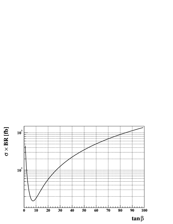
Figure 2: $\sigma\times\mathrm{BR}$ of the process $gg\rightarrow tb\mbox{$\mathrm{H}^{\pm}$}\rightarrow t\bar{t}b\bar{b}\rightarrow b\bar{b}b\bar{b}l\nu\bar{q}q^{\prime}$ for a charged Higgs mass of $\mbox{$m_{\mathrm{H}^{\pm}}$}=300\,\mbox{$\mathrm{GeV}$}$ as a function of $\tan\!\beta$.

In the following section the event generation and detector simulation are described. Section III describes the analysis which is divided into two likelihood selections presented in the sections III.2 and III.3 respectively. Section IV summarises the results, and conclusions and an outlook are given in section V.

II Event Generation and Simulation

The event generation and detector simulation for the various Monte Carlo (MC) samples used in this analysis are done within the athena framework in the atlas Software Release 6.0.3.

The signal process (1) is generated for a charged Higgs boson mass range of $\mbox{$m_{\mathrm{H}^{\pm}}$}=200-800\,\mbox{$\mathrm{GeV}$}$ using herwig 6.5 HERWIG ; HERWIGSUSY . Table 1 lists the mass points at which MC samples are produced and gives production cross sections for a set of $\tan\!\beta$ values. In the cross section calculations the factorisation and renormalisation scales, $\mu_{F}$ and $\mu_{R}$, respectively, are set to the mean transverse mass so that $\mu_{F}^{2}=\mu_{R}^{2}=\sum_{i=b,t}({p_{T}^{i}}^{2}+m_{i}^{2})/2=(m_{T}^{2}(t)+m_{T}^{2}(b))/2=\left<m_{T}^{2}\right>$. As all cross sections are calculated at leading order and no next to leading order calculations exist to date, an optimal choice of the QCD scale is not obvious. The choice of this particular scale is guided by the demand to use comparable scales in the signal and background calculations for consistency and by results obtained in gg_ttH although the process considered there can not be compared directly to the signal process considered in this report. Choosing the QCD scale is one of the main systematic uncertainties when predicting the signal and background cross sections. The value assumed here provides estimates of the cross sections to be expected but can by no means be considered as definitive. Other choices of the QCD scale or $m_{b}$ evaluation may result in cross sections differing by up to a factor 2. This topic is further discussed in section IV.

Table 1: Summary of signal MC samples for the various charged Higgs masses studied in this analysis. Inclusive and exclusive cross sections are quoted for a selection of $\tan\!\beta$ values, assuming $\mu_{F}^{2}=\mu_{R}^{2}=(m_{T}^{2}(t)+m_{T}^{2}(b))/2$ and a running $b$–quark mass. Each MC sample contains $10^{6}$ generated events.

$m_{\mathrm{H}^{\pm}}$	$\tan\!\beta$	$\sigma_{incl.}\,[pb]$	$\sigma\times\mathrm{BR}\,[pb]$
200	30	1.2	0.17
250	40	1.3	0.31
300	50	1.4	0.35
350	60	1.4	0.35
400	20	0.11	0.029
500	30	0.13	0.034
600	40	0.13	0.033
800	30	0.024	0.0063

The strong coupling constant $\alpha_{s}$ is evaluated at the 1–loop level and a running $b$–quark mass is used. A central value of $m_{t}=175\,\mbox{$\mathrm{GeV}$}$ is assumed for the top quark mass and the cteq5l parton density function is used throughout the analysis. $\mathrm{H}^{+}\rightarrow t\bar{b}$ branching ratios are evaluated with HDECAY 3.0 Djouadi:1998yw where the decay to supersymmetric particles is switched off (OFF-SUSY=1). We evaluate the branching ratios in the Maximal Mixing Scenario as described in Carena:1999xa , assuming the top quark mass mentioned above: $M_{\mathrm{SUSY}}=1\,\mathrm{TeV}$, $M_{2}=200\,\mbox{$\mathrm{GeV}$}$, $\mu=-200\,\mbox{$\mathrm{GeV}$}$, $M_{\tilde{g}}=800\,\mbox{$\mathrm{GeV}$}$ and $A_{t}=A_{b}=X_{t}+\mu/\mbox{$\tan\!\beta$}$ with $X_{t}=\sqrt{6}M_{\mathrm{SUSY}}$. The branching ratio of the $\mathrm{W}^{\pm}$ decaying to quarks is assumed to be $2/3$, and the BR to a lepton (electron or muon) plus the accompanying neutrino is taken to be $2/9$. Since each of the $\mathrm{W}^{\pm}$ can decay leptonically or hadronically, an overall factor of $2$ has to be applied. This leads to the following relation: $\sigma\times\mathrm{BR}=\sigma_{incl.}\times\mathrm{BR}(\mathrm{H}^{+}\rightarrow t\bar{b})\times 8/27.$

Samples for the background processes $gg\rightarrow t\bar{t}b\bar{b}$, $qq\rightarrow t\bar{t}b\bar{b}$ and $gg\rightarrow Z/\gamma/W\rightarrow t\bar{t}b\bar{b}$ are produced with AcerMC 1.2 Kersevan:2002dd in stand–alone mode. The QCD energy scale is chosen such that $Q^{2}_{QCD}=\Sigma({p_{T}^{i}}^{2}+m_{i}^{2})/4=\left<m^{2}_{T}\right>$. These samples are then passed to herwig 6.5 within the Athena framework for fragmentation and hadronisation. In order to study the systematic uncertainty due to different fragmentation schemes, the $gg\rightarrow t\bar{t}b\bar{b}$ sample is also passed to pythia 6.203 Sjostrand:2000wi for a similar treatment. The effect of mis–tagging light jets as $b$–jets is studied with the help of a large $t\bar{t}+\mathrm{jets}$ sample generated with herwig 6.5. Table 2 summarises the background samples and their inclusive cross sections.

Table 2: Summary of background MC samples studied in this analysis.

Process	Generator	$\sigma_{incl.}\,[pb]$	generated events
$gg\rightarrow t\bar{t}b\bar{b}$	AcerMC 1.2	10.3	$10$ M
$qq\rightarrow t\bar{t}b\bar{b}$	AcerMC 1.2	0.61	$1$ M
$gg\rightarrow Z/\gamma/W\rightarrow t\bar{t}b\bar{b}$	AcerMC 1.2	1.1	$1$ M
$t\bar{t}+\mathrm{jets}$	herwig 6.5	405.0	$50$ M

The atlas detector is simulated with the fast detector simulation atlfast as it is represented in the atlas Software Release 6.0.3. This package is based on the fortran implementation of the same package ATLFAST . Jets are reconstructed with a cone based algorithm using a cone size of $\Delta\mathrm{R}=0.4$. Only jets having a minimum transverse momentum of $p_{T}>10\,\mbox{$\mathrm{GeV}$}$ and lying in the pseudorapidity range of $|\eta|<5$ are accepted for this analysis. An efficiency of $90\,\%$ to identify isolated charged leptons is assumed. Jet energy and momentum calibration and the $b$–tagging of jets is performed within the atlfastb routine of the atlfast simulation package. The possibility to tag a jet as a $b$–jet is limited by the inner tracker acceptance range of $|\eta|<2.5$. A $b$–tagging efficiency of $60\,\%$ is assumed when simulating samples for the low luminosity option of the lhc, $50\,\%$ for the high luminosity option. Rejection factors of $\mathrm{R}_{\mathrm{c}}=10$ and $\mathrm{R}_{\mathrm{j}}=100$ are chosen for c– and light jets respectively. The $b$–tagging efficiencies and rejection factors are static, i.e. they do not depend on the pseudorapidity $\eta$ or transverse momentum $p_{T}$ of the jets. All plots and tables shown in this analysis refer to the low luminosity option of the lhc, assuming an integrated luminosity of $30\,\mathrm{fb}^{-1}$ unless explicitly stated otherwise.

II.1 Jet–Parton Matching

In order to construct and test the performance of the event reconstruction algorithm (see section III.2), it is necessary to know the link between a generated parton and a detected jet or lepton. The former is often referred to as the “Monte Carlo truth”, and the latter will be referred to as “reconstructed objects” in the following. Initially no such link between a parton and a reconstructed object is provided by the MC generator or the detector simulation program and the association is far from straightforward. In this analysis the problem is handled approximately by solving the assignment problem as described in assignmentProblem . The quantity which is minimised is the sum of all distances between the generated partons after final state radiation (FSR) and their associated reconstructed object 4–vectors. The distance between the 4–vector of a parton and the 4–vector of a reconstructed object is given by $\Delta\mathrm{R}=\sqrt{\Delta^{2}\eta+\Delta^{2}\phi}$, the distance in pseudorapidity–azimuthal angle space. If the distance between a parton and its reconstructed object exceeds $0.4$ it is assumed that no association is possible. Further, no association is attempted if any of the initial quarks after FSR has a 4–momentum outside the acceptance range of the JetMaker algorithm in atlfast.

III Analysis

The analysis has three parts. In the first step all events are required to pass a set of cuts in order to reject most of the SM background and to ensure the minimum prerequisites needed for subsequent reconstruction.

The second part is intended to find the combination of jets that correctly reconstructs the two top quarks and the charged Higgs present in the final state of the signal process. For each event the most likely correct combination is found with the help of a selection procedure described in section III.2. This likelihood is referred to as the “combinatorial likelihood”.

Once the correct combination is found for each event, a second likelihood selection, the “selection likelihood” described in section III.3, aims at separating the signal from the SM background processes.

III.1 Preselection

In the preselection, events with a topology clearly distinct from the signal topology are rejected. This ensures that only the main backgrounds discussed in section I need to be studied further. The preselection requires:

• exactly 1 isolated lepton ($l=\mathrm{e\ or}\ \mu$) with transverse momentum $p_{T}^{e}>25\,\mbox{$\mathrm{GeV}$}$, $p_{T}^{\mu}>20\,\mbox{$\mathrm{GeV}$}$ and pseudorapidity $|\eta|<2.5$,

• exactly 4 $b$–jets with $|\eta|<2.5$ and $p_{T}>20\,\mbox{$\mathrm{GeV}$}$ and

• at least 2 light jets with $|\eta|<5$ and $p_{T}>20\,\mbox{$\mathrm{GeV}$}$.

In order to trigger on the signal events the detection of a high–$p_{T}$ lepton is required. The cuts applied to the $p_{T}$ and $\eta$ of the isolated lepton are chosen such that they meet the requirements of the atlas trigger system. When running in the high luminosity option the cut on the jets’ transverse momenta is increased from $p_{T}^{\mathrm{jet}}>20\,\mbox{$\mathrm{GeV}$}$ to $p_{T}^{\mathrm{jet}}>30\,\mbox{$\mathrm{GeV}$}$. The efficiency of the precuts for signal events depends on the assumed charged Higgs mass and ranges from $1.78\,\%$ for $\mbox{$m_{\mathrm{H}^{\pm}}$}=200\,\mbox{$\mathrm{GeV}$}$ to $4.41\,\%$ for $\mbox{$m_{\mathrm{H}^{\pm}}$}=800\,\mbox{$\mathrm{GeV}$}$. The precut efficiencies are summarised in Table 3.

Table 3: Preselection efficiencies for the different charged Higgs masses studied in this analysis. The efficiencies are quoted for the low luminosity (LL) and the high luminosity (HL) option of the lhc.

$m_{\mathrm{H}^{\pm}}$ [GeV]	preselection efficiency, LL [%]	preselection efficiency, HL [%]
200	$1.783\pm 0.013$	$0.5687\pm 0.0075$
250	$3.171\pm 0.018$	$1.121\pm 0.011$
300	$3.577\pm 0.019$	$1.281\pm 0.011$
350	$3.738\pm 0.019$	$1.436\pm 0.012$
400	$3.932\pm 0.019$	$1.509\pm 0.012$
500	$4.123\pm 0.020$	$1.644\pm 0.013$
600	$4.281\pm 0.020$	$1.715\pm 0.013$
700	$4.363\pm 0.020$	(not studied)
800	$4.411\pm 0.021$	$1.872\pm 0.014$

In order to reconstruct the leptonically decaying $\mathrm{W}^{\pm}$ ($\mathrm{W}^{\pm}_{\mathrm{lep}}$) the 4–momentum of the daughter neutrino needs to be reconstructed. The x– and y–components of the neutrino momentum are assumed to coincide with the measured missing transverse momentum components $p_{x}^{\mathrm{miss}}$ and $p_{y}^{\mathrm{miss}}$ respectively. The z–component however can not be measured but must be calculated by solving the equation:

$$m_{\mathrm{W}^{\pm}}^{2}=(E_{\nu}+E_{l})^{2}-(\vec{p}_{\nu}+\vec{p}_{l})^{2},\mathrm{\ \ \ with\ \ }E_{\nu}=|\vec{p_{\nu}}|.$$

This equation can result in two or zero real solutions for $p_{\nu}^{z}$. If two solutions are found, both are kept for later evaluation in the event reconstruction algorithm. However, in approximately $25\,\%$ of the events no solution is found. In order to keep these events and still be able to reconstruct the leptonically decaying $\mathrm{W}^{\pm}_{\mathrm{lep}}$ in those otherwise fatal cases, the collinear approximation approach described in jochen is adopted: $p_{\nu}^{z}=p_{l}^{z}$ is assumed if no solution can be found, and the resulting $\mathrm{W}^{\pm}$ 4–momentum is rescaled to match $m_{\mathrm{W}^{\pm}}$. This increases the $\mathrm{W}^{\pm}_{\mathrm{lep}}$ reconstruction efficiency from $75\,\%$ to $100\,\%$ and only a small loss in the resolution of the reconstructed leptonically decaying $\mathrm{t}_{\mathrm{lep}}$ is observed.

III.2 The Combinatorial Likelihood

The final state of the signal process (1) is quite complex, featuring four $b$–jets, two light jets from the hadronically decaying $\mathrm{W}^{\pm}$($\mathrm{W}^{\pm}_{\mathrm{had}}$) and an isolated lepton plus missing transverse momentum from the leptonically decaying $\mathrm{W}^{\pm}$($\mathrm{W}^{\pm}_{\mathrm{lep}}$). Quark and gluon jets from initial and final state radiation and the underlying event are also present, increasing the jet multiplicity. Initially it is unknown which reconstructed objects should be combined to reconstruct the two $\mathrm{W}^{\pm}$s, the two top quarks, and finally the charged Higgs boson. The combinatorial likelihood aims at identifying the correct reconstructed objects to combine and thereby making the correct reconstruction of the whole event possible. In order to incorporate as much information available from each event as possible a multivariate technique is chosen to find the correct combination of reconstructed objects for each event. We choose to implement a likelihood selection distinguishing two classes where the first class represents the correct combination and the second class all the wrong ones. The likelihood formalism used in this analysis is outlined briefly in the following, generalising to $n$ classes of events:

For each of the $m$ observables $x_{i}$ used to distinguish between the $n$ classes, the normalised probability density functions (pdf)

$$f_{i}^{j}(x_{i}),\qquad\text{ where }i=1,\dots,m\text{ and }j=1,\dots,n$$ (5)

have to be determined. The probability that an event belongs to class $j$ when measuring the value $x_{i}$ for variable $i$ is given by

$$p_{i}^{j}(x_{i})=\frac{f_{i}^{j}(x_{i})}{\sum^{n}_{k=1}f_{i}^{k}(x_{i})}.$$ (6)

The likelihood ${\cal L}$ that an event belongs to class j when measuring $m$ variables $x_{1},\dots,x_{m}$ is then given by the normalised product of the probabilities Eq. 6 over all $m$ variables:

$${\cal L}^{j}=\frac{\displaystyle\prod^{m}_{l=1}p_{l}^{j}(x_{l})}{\displaystyle\sum^{n}_{k=1}\prod^{m}_{l=1}p_{l}^{k}(x_{l})}.$$ (7)

The likelihood has values in the range 0,…,1. Information about possible correlations between the input variables is neglected by this procedure.

When constructing the pdfs for the combinatorial likelihood it is essential to know the correct association of partons to reconstructed objects as described in section II.1. The fraction of signal events passing the precuts for which a valid association to partons is found depends on the charged Higgs mass and ranges from $45\,\%$ at $\mbox{$m_{\mathrm{H}^{\pm}}$}=200\,\mbox{$\mathrm{GeV}$}$ to $58\,\%$ at $\mbox{$m_{\mathrm{H}^{\pm}}$}=800\,\mbox{$\mathrm{GeV}$}$. Only events having a valid parton association can be used to obtain the pdfs for the correct– and the wrong–combination class.

Any algorithm used to reconstruct the events has a chance to find the correct combination only if the correct four jets are $b$–tagged and the two light jets originating from the hadronically decaying $\mathrm{W}^{\pm}$ pass the precut constraints. Of those events passing the precuts and obtaining a valid association to partons, only approximately $65\,\%$ fulfill this requirement. This means that for $\approx 35\,\%$ of signal events passing the precuts the completely correct reconstruction is doomed from the beginning.

The combinatorial likelihood is based on the following $9$ variables, where the labelling of partons in the signal process is illustrated in Figure 3:

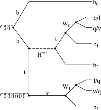
Figure 3: One of the possible Feynman diagrams for the signal process $gg\rightarrow tb\mbox{$\mathrm{H}^{\pm}$}\rightarrow b\bar{b}b\bar{b}l\nu\bar{q}q^{\prime}$, illustrating the labelling of the partons adopted in this analysis.

1. $m_{jj}$: the invariant mass of any two light jets. For the correct combination this mass should be within the $\mathrm{W}^{\pm}$ mass peak around $\mbox{$m_{\mathrm{W}^{\pm}}$}=80.4\,\mbox{$\mathrm{GeV}$}$ whereas the distribution of invariant masses of pairs of jets not originating from a $\mathrm{W}^{\pm}$ is rather flat.

2. $m_{jjb}$: the invariant mass of any two light jets and one of the four $b$–jets. The correct combination should reproduce the top mass. This variable aims at correctly reconstructing the hadronically decaying top quark $\mathrm{t}_{\mathrm{had}}$.

3. $m_{l{\nu}b}$: the invariant mass of the isolated lepton, one solution for the neutrino reconstructed as described in III.1 and one of the $b$–jets. This variable aims at reconstructing the leptonically decaying top quark $\mathrm{t}_{\mathrm{lep}}$.

4. $p_{T}(b_{2})$: the $p_{T}$ of the $b$–jet assumed to originate from the charged Higgs decay.

5. $p_{T}(b_{0})$: the $p_{T}$ of the assumed companion $b$–jet produced in the $gg\rightarrow tb\mbox{$\mathrm{H}^{\pm}$}$ process.

6. $\Delta\mathrm{R}(j,j)$: $\Delta\mathrm{R}$ between any two light jets. Like $m_{jj}$ this variable helps to reconstruct $\mathrm{W}^{\pm}_{\mathrm{had}}$.

7. $\Delta\mathrm{R}(jj,b)$: $\Delta\mathrm{R}$ between the sum of any two light jets and a $b$–jet. Like $m_{jjb}$ this variable is related to the reconstruction of $\mathrm{t}_{\mathrm{had}}$.

8. $\Delta\mathrm{R}(l,b)$: $\Delta\mathrm{R}$ between the isolated lepton and a $b$–jet. Like $m_{l{\nu}b}$ this variable aims at reconstructing $\mathrm{t}_{\mathrm{lep}}$.

9. $\Delta\mathrm{R}(b_{2},t_{1})$: $\Delta\mathrm{R}$ between the $b$–jet and the top quark candidate originating from the charged Higgs decay. For the top quark candidate all possible modes of reconstructing a top quark are considered.

The probability density functions for the nine variables used in the combinatorial likelihood are shown in Figure 4 for a charged Higgs mass of $400\,\mbox{$\mathrm{GeV}$}$. Overflow bins are included in the normalisation of the histograms and used when calculating the combinatorial likelihood output.

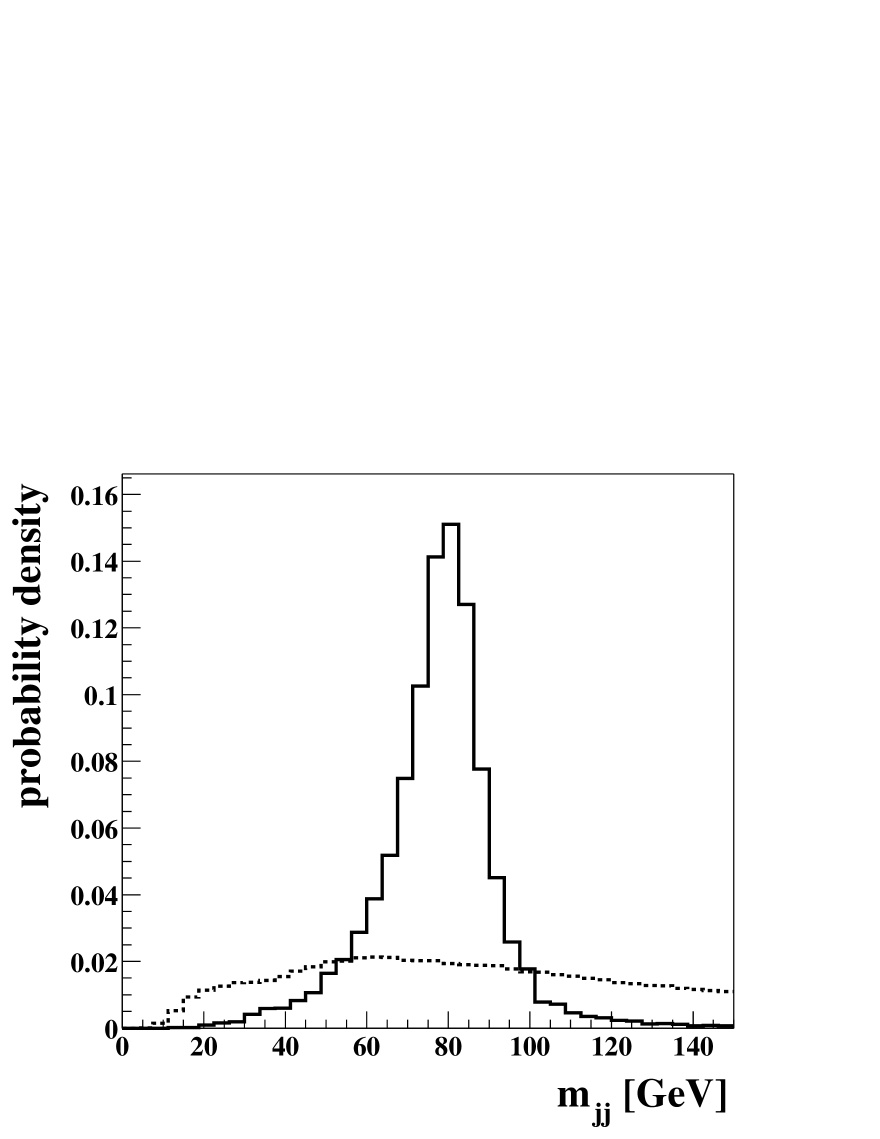
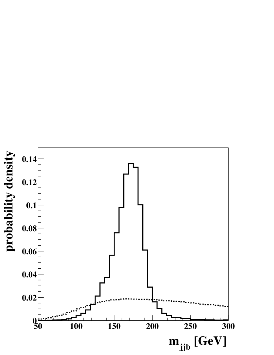
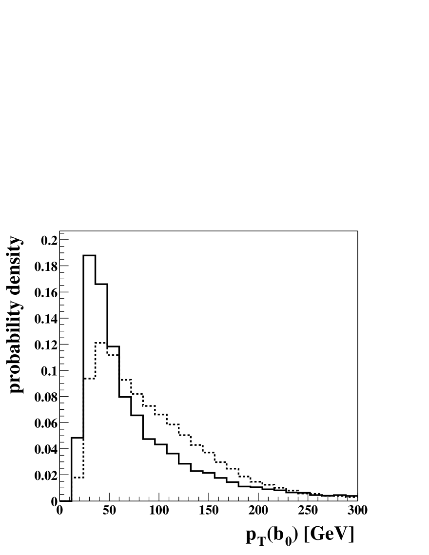
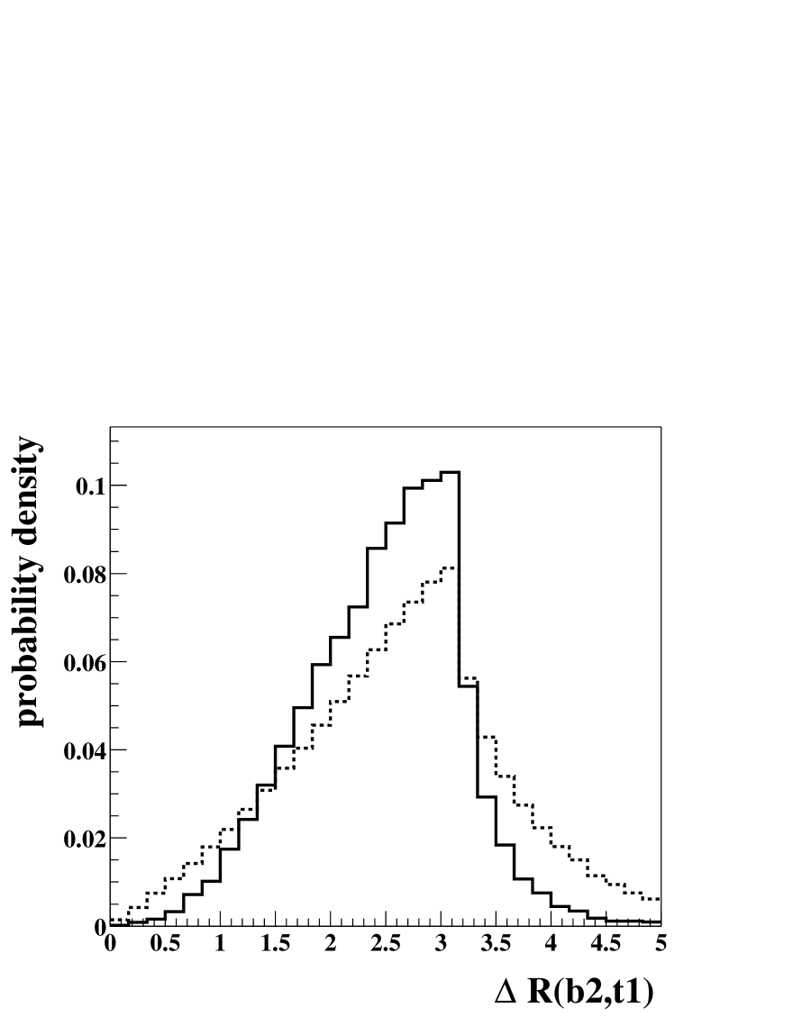
Figure 4: The probability density functions for the nine variables used in the combinatorial likelihood for a charged Higgs mass of $\mbox{$m_{\mathrm{H}^{\pm}}$}=400\,\mbox{$\mathrm{GeV}$}$. All distributions are normalised to unity including overflow bins. Correct combinations are represented by a solid line, all wrong combinations by a dashed line.

The corresponding normalised likelihood distributions for the correct–combination class are shown in Figure 5 for the correct combination and all the wrong ones. As expected, the distribution corresponding to the correct combination peaks at $1$ whereas the distribution representing all the wrong combinations peaks at $0$. However, it is important to note the tail in the distribution representing the wrong combinations up to high likelihood values. The total number of combinations of the reconstructed objects to reconstruct the event completely is given by

$$N=4!\times\left(\begin{array}[]{c}m\\ 2\end{array}\right)\times N_{\nu}\times 2,$$

where $m$ is the number of light jets in the event and $N_{\nu}$ is the number of solutions for the neutrino. The $4!$ represents the number of possibilities to order the four $b$–jets and the factor of $2$ reflects the possible associations of $\mathrm{W}^{\pm}_{\mathrm{lep}}$ and $\mathrm{W}^{\pm}_{\mathrm{had}}$ to the top quarks. This number $N$ depends on the number of light jets in the event and is generally quite large. Hence the number of wrong combinations is large and the possibility of one of those wrong combinations having a combinatorial likelihood output higher than the correct combination is not negligible, thus reducing the probability of identifying the correct combination.

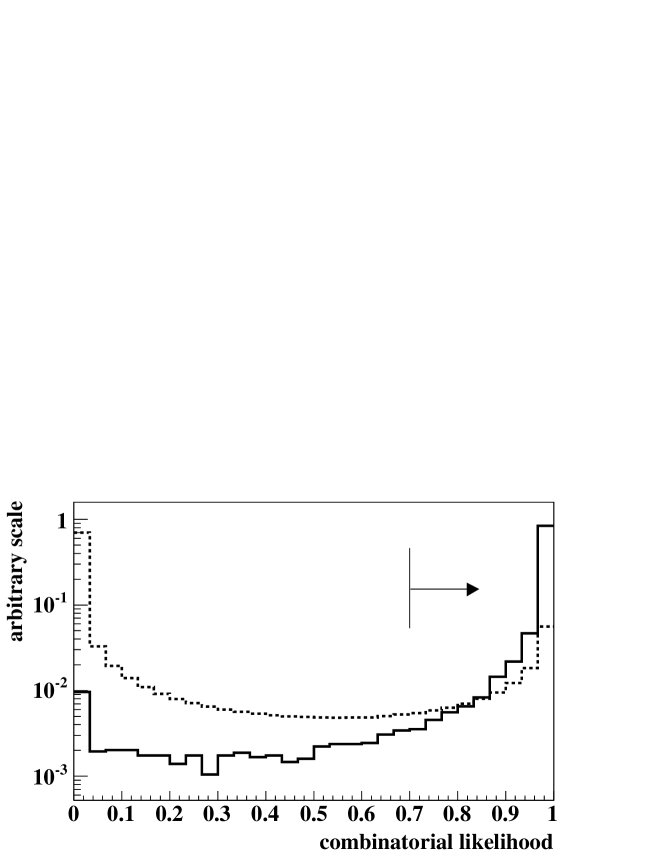
Figure 5: The normalised combinatorial likelihood output distributions for the correct–combination class. The correct (solid) and the wrong (dashed) combinations are shown for a charged Higgs mass of $\mbox{$m_{\mathrm{H}^{\pm}}$}=400\,\mbox{$\mathrm{GeV}$}$. Only combinations with a likelihood output larger than $0.7$ are accepted.

For each event the combination yielding the highest correct–combination likelihood is treated as the correct combination. Nevertheless, if this selected combination yields a likelihood value below $0.7$ the event is rejected. The efficiency of this cut varies between $90\,\%$ for $\mbox{$m_{\mathrm{H}^{\pm}}$}=200\,\mbox{$\mathrm{GeV}$}$ and $95\,\%$ for $\mbox{$m_{\mathrm{H}^{\pm}}$}=800\,\mbox{$\mathrm{GeV}$}$ for the signal process and is approximately $85\,\%$ for the main $gg\rightarrow t\bar{t}b\bar{b}$ background.

The performance of the combinatorial likelihood is checked using the Monte Carlo truth information to associate the final state partons with the reconstructed objects as described in section II.1. An event is classified as correctly reconstructed if the four $b$–jets and the two light jets are correctly associated with their corresponding final state partons and the correct lepton is found to be isolated. Some performance benchmarks of the combinatorial likelihood are shown in Figure 6 as a function of the charged Higgs boson mass.

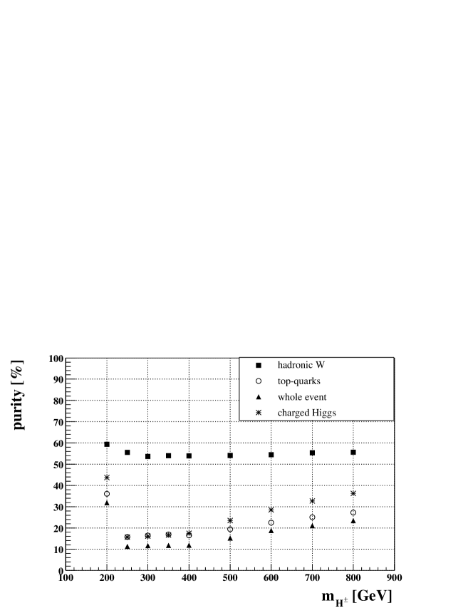
Figure 6: Purity of the combinatorial likelihood in reconstructing the hadronically decaying $\mathrm{W}^{\pm}$ (squares), the two top quarks (circles), the charged Higgs boson (stars) and the whole event (triangles) over the considered charged Higgs mass range.

The squares indicate the fraction of correctly reconstructed hadronically decaying $\mathrm{W}^{\pm}$, referred to as purity in the following. This purity does not depend strongly on the charged Higgs mass and lies between $53\,\%$ and $60\,\%$. The purity of reconstructing the two top quarks is represented by the open circles. Here the purity depends strongly on $m_{\mathrm{H}^{\pm}}$ and rises to values above $25\,\%$ only for charged Higgs masses either very close to $m_{\mathrm{t}}$ or for $\mbox{$m_{\mathrm{H}^{\pm}}$}\geq 700\,\mbox{$\mathrm{GeV}$}$. Similar behaviour can be seen for the purity of the charged Higgs boson (stars) and the whole event reconstruction (triangles). The only variables used in the combinatorial likelihood that depend strongly on $m_{\mathrm{H}^{\pm}}$  are variables $4$ and $9$. The $p_{T}$ of the $b$–jet from the charged Higgs decay depends strongly on the mass of the charged Higgs boson and is well separated from the average $p_{T}$ of the other $b$–jets in the event only for very small or quite large charged Higgs masses. A similar statement applies to the distance $\Delta\mathrm{R}(b_{2},t_{1})$ between the top quark and the $b$–quark originating from the charged Higgs decay. A light charged Higgs boson is produced with a sizable boost and its decay products will have a small distance in $\Delta\mathrm{R}$–space. On the other hand, a heavy charged Higgs boson is produced nearly at rest and hence the distance between its decay products will be large. The mass dependence of the performance of the combinatorial likelihood is mainly determined by the mass dependence of variables $4$ and $9$.

It should be noted that in the mass region $\mbox{$m_{\mathrm{H}^{\pm}}$}=250\,$–$\,600\,\mbox{$\mathrm{GeV}$}$ the purity of the charged Higgs reconstruction does not exceed $30\,\%$. As a consequence the reconstructed charged Higgs mass is substantially blurred by the combinatorial background. Hence the detection of a clear mass peak in the reconstructed charged Higgs mass distribution is difficult. The correct reconstruction of the whole event is important for the performance of the selection likelihood discussed below, since it relies on the correct association of reconstructed objects to the charged Higgs boson and the top quarks. The ability to distinguish signal from background processes is already diminished by the imperfect performance of the combinatorial likelihood.

Before combining a $\mathrm{W}^{\pm}$ and a $b$–quark to form a reconstructed top quark, the $\mathrm{W}^{\pm}$ 4–momentum is scaled to reproduce $m_{\mathrm{W}^{\pm}}=80.4\,\mbox{$\mathrm{GeV}$}$. The reconstructed hadronic $\mathrm{W}^{\pm}$ and the two reconstructed top masses for events passing the cut of $0.7$ on the combinatorial likelihood output are shown in Figure 7.

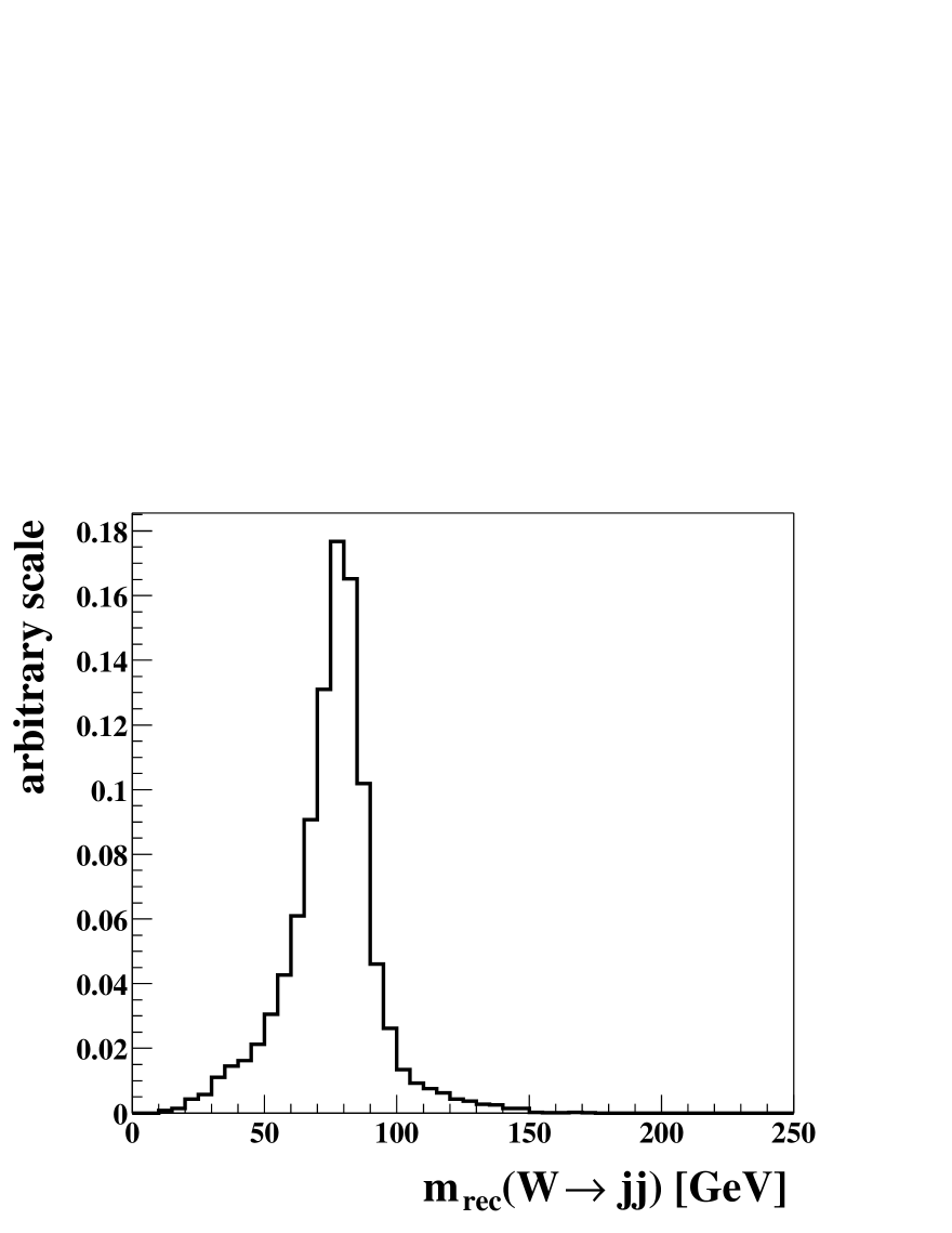
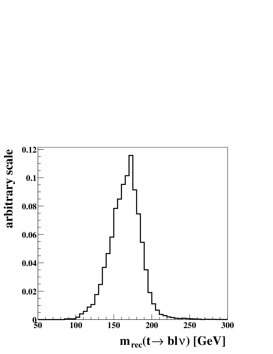
Figure 7: Reconstructed masses for the hadronically decaying $\mathrm{W}^{\pm}$ and the hadronic and leptonic top quark for events passing the cut on the combinatorial likelihood. The signal is generated assuming $\mbox{$m_{\mathrm{H}^{\pm}}$}=400\,\mbox{$\mathrm{GeV}$}$.

Reconstructed charged Higgs masses are shown for $\mbox{$m_{\mathrm{H}^{\pm}}$}=200$, $400$ and $800\,\mbox{$\mathrm{GeV}$}$ in Figure 8. The solid line represents the reconstructed mass obtained with the combinatorial likelihood. To predict the detector performance and to illustrate the effect of the combinatorial background the same distributions are also shown using the Monte Carlo truth information to select the correct combination of reconstructed objects as the dashed lines. The effect of the combinatorial background is clearly visible as a tail in the reconstructed charged Higgs mass distribution, especially toward higher reconstructed masses. For higher charged Higgs masses detector effects become more prominent. Even when the MC truth information is included a large tail toward lower reconstructed masses develops.

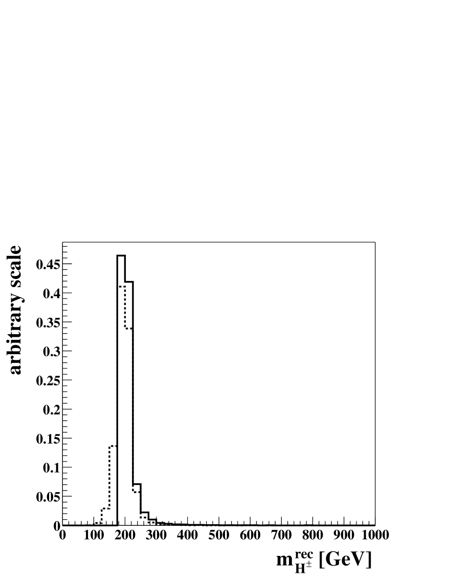
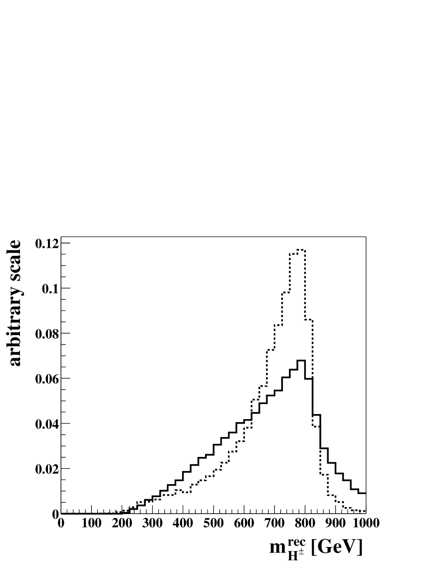
Figure 8: Reconstructed charged Higgs masses for $\mbox{$m_{\mathrm{H}^{\pm}}$}=200$, $400$ and $800\,\mbox{$\mathrm{GeV}$}$. The solid line shows the reconstructed mass as obtained with the combinatorial likelihood. The dashed line illustrates the charged Higgs mass resolution obtained when utilizing the Monte Carlo truth information to match the tree–level partons to the reconstructed objects.

III.3 The Selection Likelihood

To enhance the signal and suppress the Standard Model background a second likelihood selection is implemented. The selection likelihood distinguishes three classes of events: 1) the $gg\rightarrow tb\mbox{$\mathrm{H}^{\pm}$}$ signal process, 2) the $gg/qq\rightarrow t\bar{t}b\bar{b}$ background, and 3) the $gg\rightarrow Z/\gamma/W\rightarrow t\bar{t}b\bar{b}$ background process and is implemented using the same formalism as described in section III.2. It exploits differences between the distributions of the signal and the Standard Model backgrounds in the following four variables:

1. $m_{b_{0}b_{2}}$: the invariant mass of the two $b$–jets not originating from a top quark decay. In the signal events one of the jets originates from a heavy charged Higgs boson whereas in the background processes both $b$–jets originate from gluon splitting. Hence the invariant mass of the two jets is expected to be lower in background than in signal events.

2. $\cos\theta(b_{0},b_{2})$: the cosine of the angle between the two $b$–jets not originating from a top quark decay. Since the two $b$–jets originate from gluon splitting for the background processes they are expected to be collinear whereas the distribution should be flat for the signal process.

3. $\cos\theta(b_{0}+b_{2})$: the cosine of the azimuthal angle of the $b_{0}+b_{2}$ jet system.

4. $\cos\theta(t_{\mathrm{boost}},\mbox{$\mathrm{H}^{\pm}$}_{\mathrm{recon}})$: the cosine of the angle between the reconstructed charged Higgs boson momentum and the reconstructed top quark associated with its decay, where the reconstructed top quark 4–momentum is boosted into the charged Higgs boson rest frame.

The corresponding probability density distributions are shown in Figure 9 for $m_{\mathrm{H}^{\pm}}$=600 $\mathrm{GeV}$.

Variables related to transverse momenta or invariant masses of jet systems tend to shift the background peak in the reconstructed charged Higgs mass distribution towards the nominal charged Higgs mass. Therefore only variables involving angular correlations are used in the selection likelihood. The only exception is $m_{b_{0}b_{2}}$ for which it has been demonstrated that no such shift occurs for cuts of less than $0.4$ on the resulting selection likelihood.

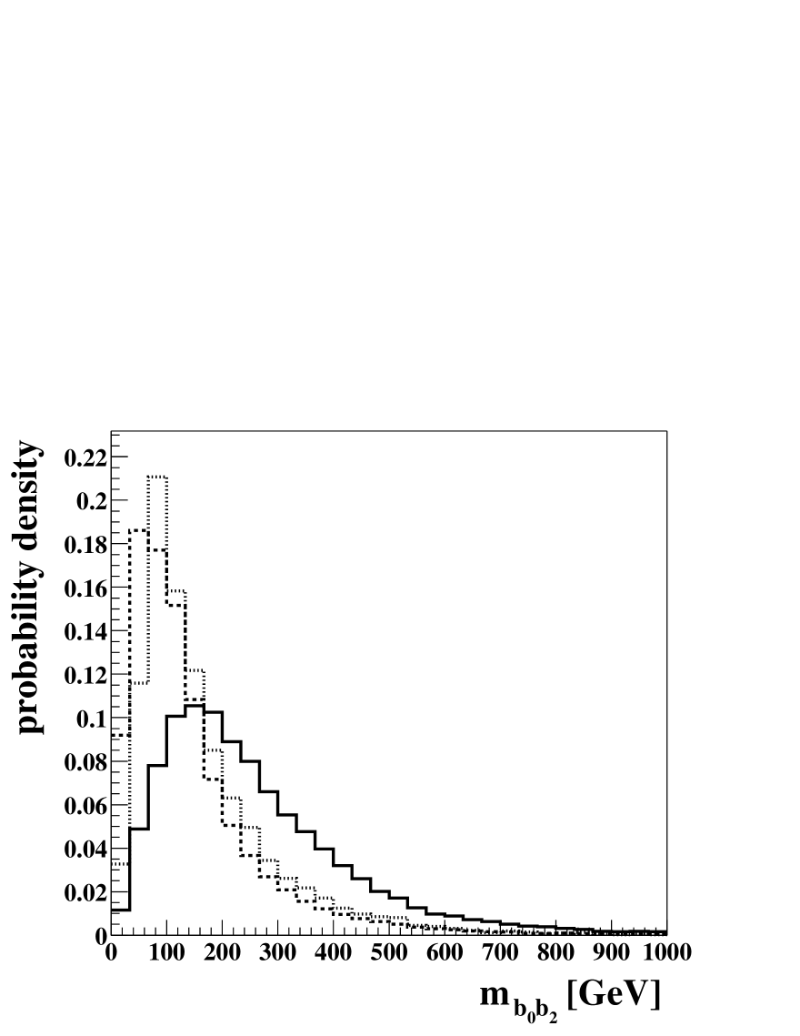
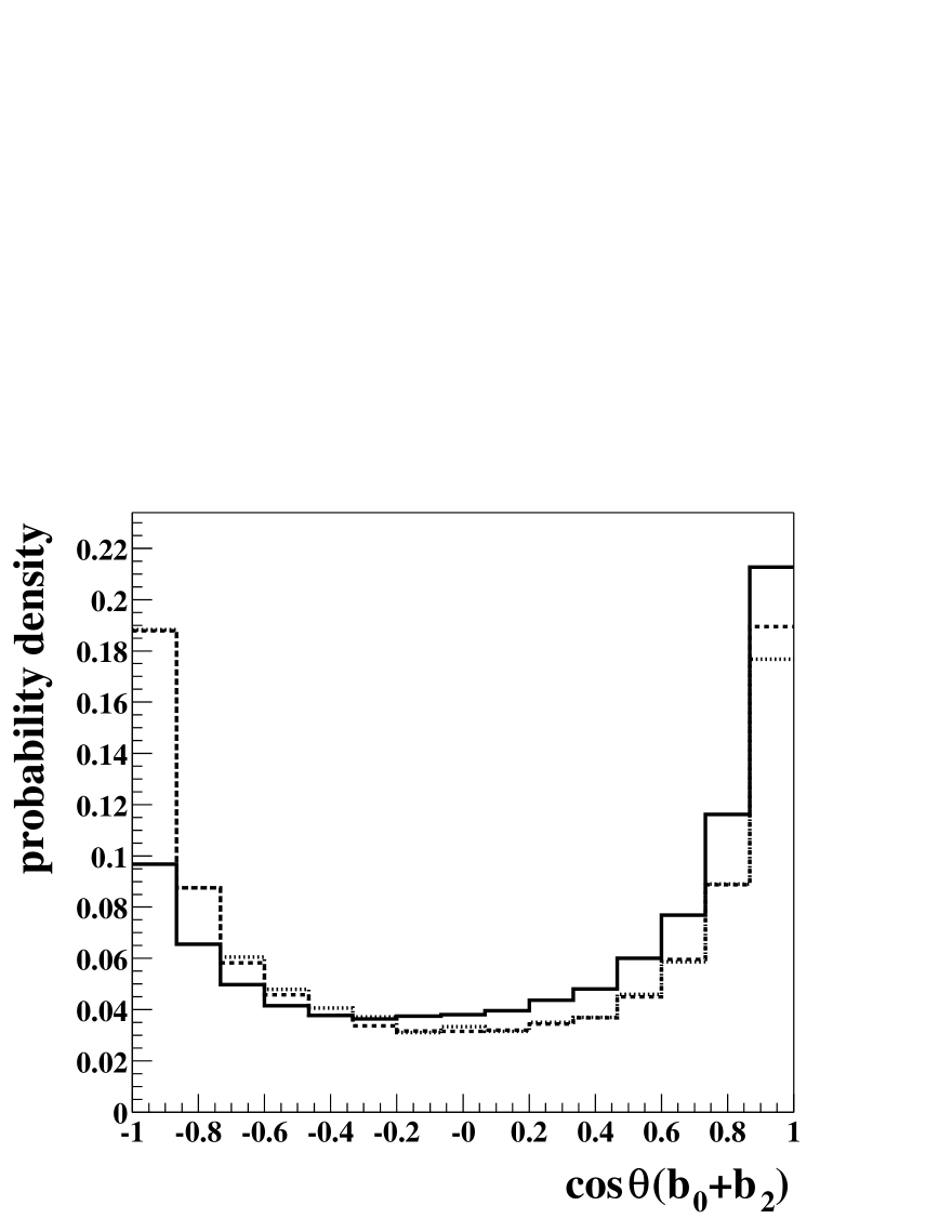
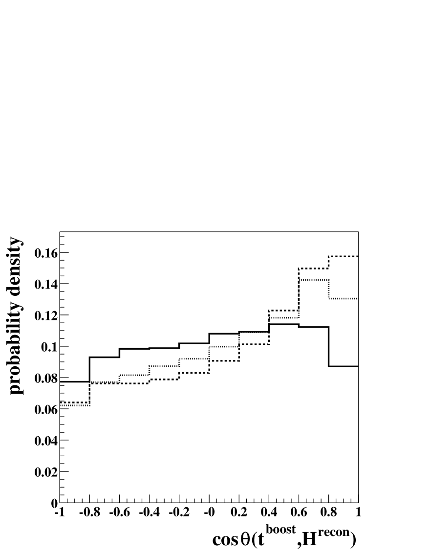
Figure 9: The probability density functions for the four variables used in the selection likelihood for a charged Higgs mass of $\mbox{$m_{\mathrm{H}^{\pm}}$}=600\,\mbox{$\mathrm{GeV}$}$. All distributions are normalised to unity. For each variable the distributions corresponding to the $gg\rightarrow tb\mbox{$\mathrm{H}^{\pm}$}$ signal process (solid), the $gg/qq\rightarrow t\bar{t}b\bar{b}$ background process (dashed) and the electroweak $gg\rightarrow Z/\gamma/W\rightarrow t\bar{t}b\bar{b}$ process (dotted) are shown.

The normalised selection likelihood output distributions for the signal class and assuming $\mbox{$m_{\mathrm{H}^{\pm}}$}=600\,\mbox{$\mathrm{GeV}$}$ are shown in Figure 10. These distributions are calculated for each charged Higgs mass under consideration.

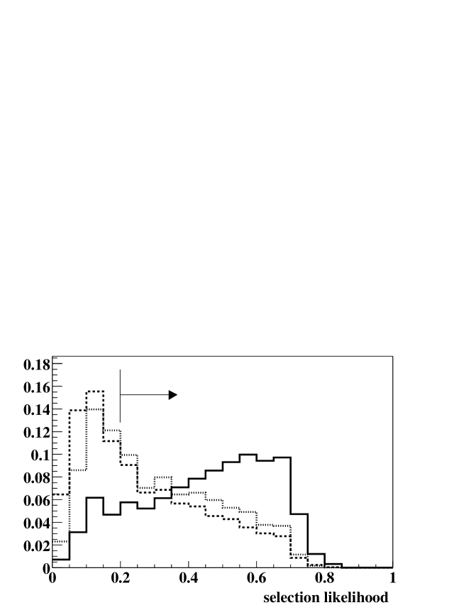
Figure 10: The normalised selection likelihood output distributions for the signal class. Distributions for the $gg\rightarrow tb\mbox{$\mathrm{H}^{\pm}$}$ signal process (solid), the $gg/qq\rightarrow t\bar{t}b\bar{b}$ background process (dashed) and the electroweak $gg\rightarrow Z/\gamma/W\rightarrow t\bar{t}b\bar{b}$ process (dotted) are shown for a charged Higgs mass of $\mbox{$m_{\mathrm{H}^{\pm}}$}=600\,\mbox{$\mathrm{GeV}$}$. Only events yielding a selection likelihood output larger than $0.2$ are selected.

Signal events are separated from the Standard Model background by selecting only those events yielding a selection likelihood output larger than $0.2$. This optimal cut value is found by varying the cut on the likelihood output in steps of $0.05$ and requiring the method to yield the highest discovery potential over the selected range of charged Higgs masses. Figure 11 shows the resulting reconstructed charged Higgs mass distribution for a choice of charged Higgs masses. Here an integrated luminosity of ${\cal L}=30\,\mathrm{fb}^{-1}$ and $\mbox{$\tan\!\beta$}=80$ is assumed. Only a slight shift of the peak in the reconstructed charged Higgs boson mass for the backgrounds is observed for growing $m_{\mathrm{H}^{\pm}}$. For $\mbox{$m_{\mathrm{H}^{\pm}}$}\gtrsim 400\,\mbox{$\mathrm{GeV}$}$ the peaks in the reconstructed charged Higgs mass for the signal and the background processes can be separated.

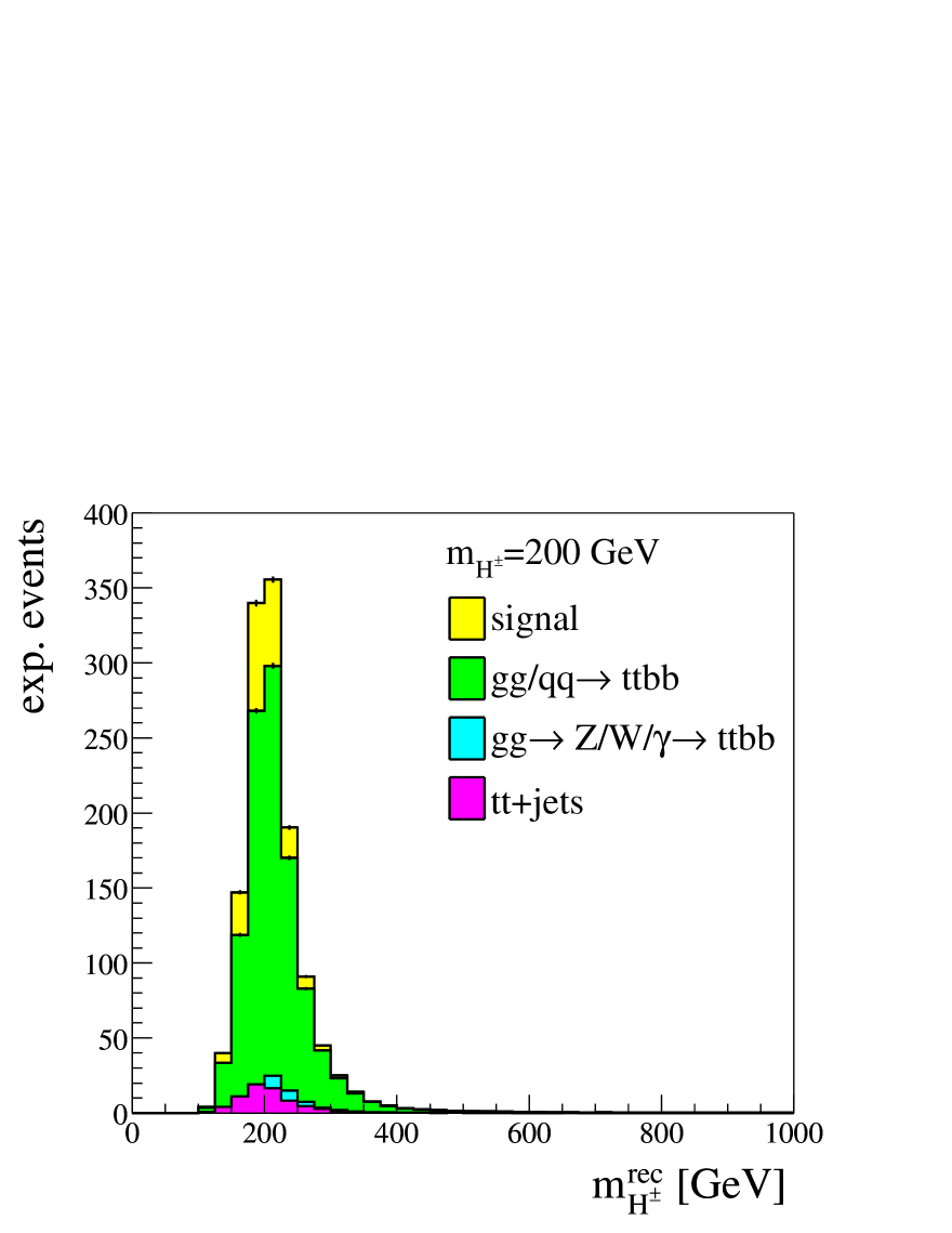
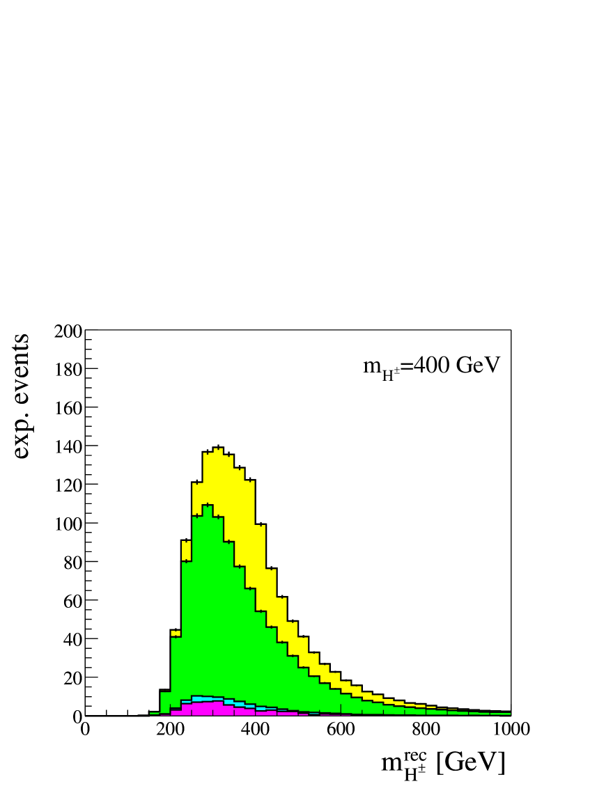
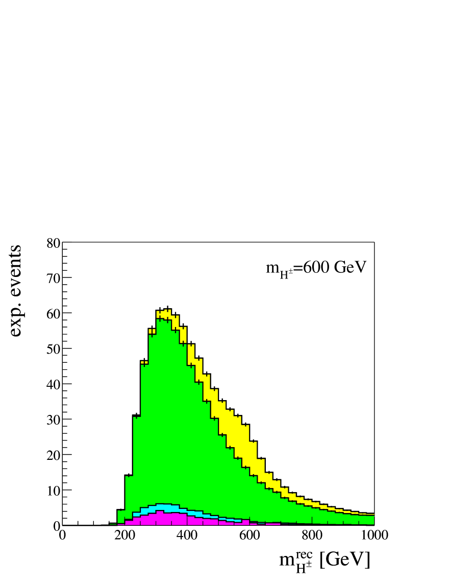
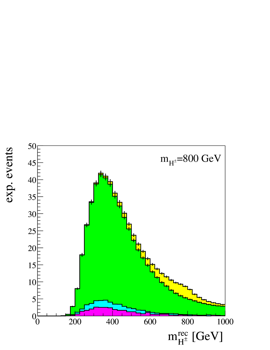
Figure 11: Reconstructed charged Higgs masses for $\mbox{$m_{\mathrm{H}^{\pm}}$}=200$, $400$, $600$ and $800\,\mbox{$\mathrm{GeV}$}$ and $\mbox{$\tan\!\beta$}=80$. The histograms are normalised to the expected event rate for ${\cal L}=30\,\mathrm{fb}^{-1}$. The $gg\rightarrow tb\mbox{$\mathrm{H}^{\pm}$}$ signal process (yellow) is shown on top of the Standard Model backgrounds $gg/qq\rightarrow t\bar{t}b\bar{b}$ (green), $gg\rightarrow Z/\gamma/W\rightarrow t\bar{t}b\bar{b}$ (light blue) and $t\bar{t}+\mathrm{jets}$ (pink).

All events within a mass window of $\pm 100\,\mbox{$\mathrm{GeV}$}$ around the nominal charged Higgs mass are selected. The width of the mass window has little influence on the discovery potential and hence is not optimised. The number of selected signal and background events is then treated like in a simple counting experiment and the Poisson significance is calculated for each charged Higgs mass and value of $\tan\!\beta$. The resulting $5\,\sigma$ discovery contour is presented and discussed in the next section.

Figure 12 summarises the signal selection efficiency and the expected number of background events after all cuts have been made for the whole range of charged Higgs masses studied. The signal selection efficiency lies within $1.4-2.7\,\%$ and reaches its maximum around $\mbox{$m_{\mathrm{H}^{\pm}}$}\approx 300\,\mbox{$\mathrm{GeV}$}$.

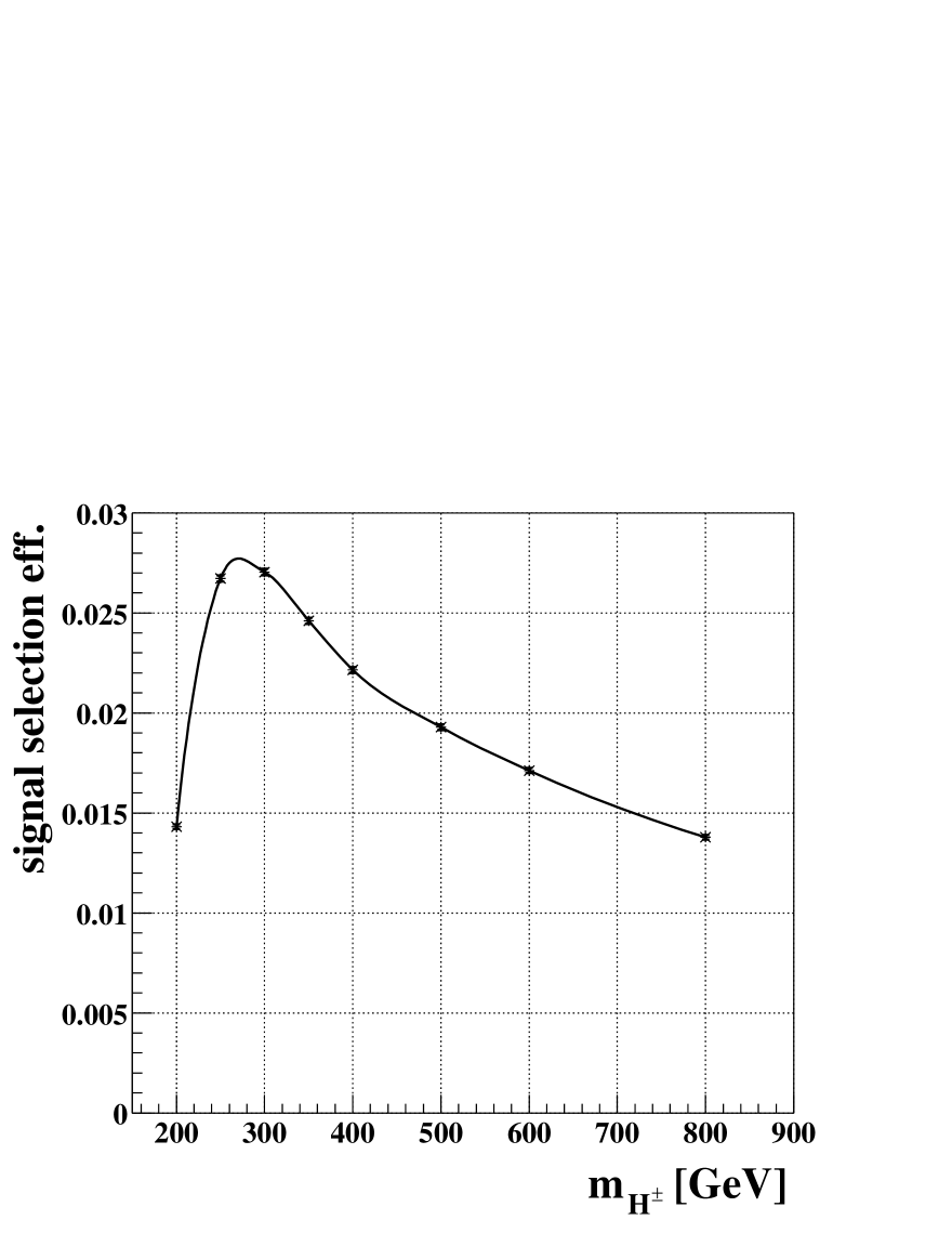
Figure 12: The signal selection efficiency and the total expected number of background events after all cuts in the mass window of $\pm 100\,\mbox{$\mathrm{GeV}$}$ assuming an integrated luminosity of $30\,\mathrm{fb}^{-1}$. The dots represent the charged Higgs masses that were studied, and the line is a smooth interpolation.

IV Results

The results of the analysis are described in this section in terms of $5\,\sigma$ discovery contours in the $(m_{\mathrm{A}},\mbox{$\tan\!\beta$})$ plane. They are presented for integrated luminosities of $30\,\mathrm{fb}^{-1}$ for the low luminosity option and $300\,\mathrm{fb}^{-1}$ for the high luminosity option of the lhc. In the latter case a $b$–tag efficiency of $\epsilon_{b}=0.5$ is assumed and the $p_{T}^{\mathrm{min}}$ cut on all jets is raised to $p_{T}^{\mathrm{jet}}>30\,\mbox{$\mathrm{GeV}$}$. The degradation of jet–energy measurements due to pile–up is taken approximately into account by choosing the high luminosity option in the atlfast simulation package. Figure 13 shows the expected discovery contours taking no systematic uncertainties into account. The charged Higgs boson can be detected for $\tan\!\beta$ values down to $35$ for $\mbox{$m_{\mathrm{H}^{\pm}}$}\approx 250\,\mbox{$\mathrm{GeV}$}$ based on an integrated luminosity of $30\,\mathrm{fb}^{-1}$. For the high luminosity option and $300\,\mathrm{fb}^{-1}$ the reach in $\tan\!\beta$ goes down to approximately $28$ for the same charged Higgs mass region. The analysis presented here depends heavily on the $b$–tagging performance and the reconstruction of jets with a relatively low $p_{T}$. This explains why only a small improvement in the discovery potential is observed when switching to the high luminosity option.

Figure 13: The $5\,\sigma$ discovery contours for the process $gg\rightarrow tb\mbox{$\mathrm{H}^{\pm}$}\rightarrow t\bar{t}b\bar{b}\rightarrow b\bar{b}b\bar{b}l\nu\bar{q}q^{\prime}$ in the $(m_{\mathrm{A}},\mbox{$\tan\!\beta$})$ plane for the low and the high luminosity option of the lhc, assuming integrated luminosities of $30\,\mathrm{fb}^{-1}$ and $300\,\mathrm{fb}^{-1}$ respectively. A common renormalisation and factorisation scale of $\mu_{F}^{2}=\mu_{R}^{2}=(m_{T}^{2}(t)+m_{T}^{2}(b))/2$ and a running $b$–quark mass are assumed when evaluating the cross sections of the various processes involved. No systematic uncertainties are taken into account.

The uncertainty in the prediction of the signal and background cross sections due to the choice of QCD scale and running or pole $b$–quark masses is quite large as already discussed in section II. Figure 14 shows some cross section predictions

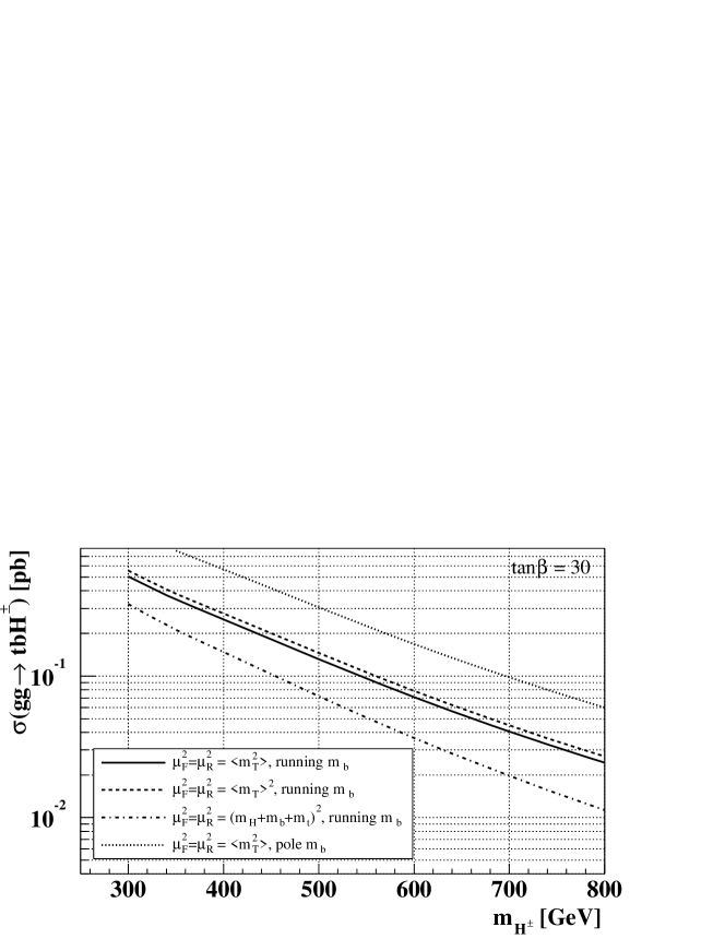
Figure 14: cross section predictions for the $gg\rightarrow tb\mbox{$\mathrm{H}^{\pm}$}$ process obtained with herwig $6.5$ assuming different QCD scales and $b$–quark mass evaluations. A value of $\mbox{$\tan\!\beta$}=30$ is chosen.

obtained with herwig 6.5 for the $gg\rightarrow tb\mbox{$\mathrm{H}^{\pm}$}$ process, assuming different QCD scales and $m_{b}$ evaluations. The lower three curves represent cross section predictions for a running $b$–quark mass and renormalisation and factorisation scales of $\mu_{F}^{2}=\mu_{R}^{2}=(m_{T}(t)+m_{T}(b))^{2}/4$, $(m_{T}^{2}(t)+m_{T}^{2}(b))/2$, and $(\mbox{$m_{\mathrm{H}^{\pm}}$}+m_{t}+m_{b})^{2}$. Whereas only a small difference is observed between the predictions of the first two choices, a rather large reduction in the expected signal cross section is observed if a QCD scale of $\mbox{$m_{\mathrm{H}^{\pm}}$}+m_{b}+m_{t}$ is assumed. However, NLO calculations for the $2\rightarrow 2$ process $gb\rightarrow t\mbox{$\mathrm{H}^{\pm}$}$ Plehn:2002vy and the $gg\rightarrow t\bar{t}H$ process gg_ttH show that this choice of scale might be too high. The same studies show also that the cross sections are likely to be overestimated when using a pole $b$–quark mass. We therefore adopt a running $b$–mass, ensuring K–factors larger than 1. To illustrate the effect of a larger signal cross section prediction we nevertheless show the cross sections expected when assuming a $b$–quark pole mass in the uppermost curve in Figure 14 and the corresponding improvement in the discovery contour in Figure 15 (left plot). The latter plot shows that improvements in the discovery potential due to K–factors $>1$ might be sizable.

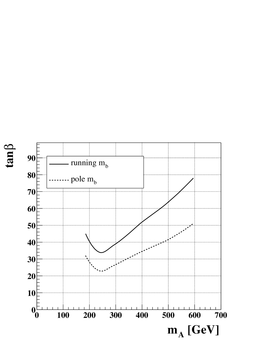
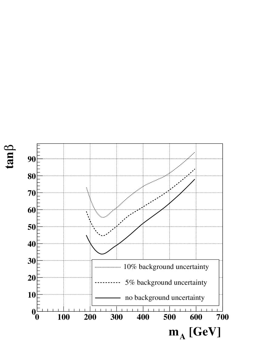
Figure 15: Influences of systematic uncertainties on the discovery potential assuming an integrated luminosity of $30\,\mathrm{fb}^{-1}$ and $\mu_{F}^{2}=\mu_{R}^{2}=(m_{T}^{2}(t)+m_{T}^{2}(b))/2$. The left plot shows the improvement in discovery potential if a pole $b$–quark mass is assumed instead of a running $m_{b}$ when evaluating the $gg\rightarrow tb\mbox{$\mathrm{H}^{\pm}$}$ cross section. The right plot shows $5\,\sigma$ discovery contours taking systematic uncertainties on the background cross section normalisation of $5\,\%$ and $10\,\%$ into account. Here a running $m_{b}$ is used.

The main $gg/qq\rightarrow t\bar{t}b\bar{b}$ background cross section prediction is also very sensitive to the QCD scale Kersevan:2002dd and the uncertainties on the cross section prediction are of the same order as for the signal process. However, here we will assume that the background cross section can be measured using side–bands in the reconstructed mass distribution which are relatively signal–free. The precision of this procedure depends on the charged Higgs mass and on the integrated luminosity available. No detailed study is conducted here, but to give some indication of how the discovery potential is affected by this uncertainty on the expected Standard Model background, we assume an uncertainty of $5$–$10\,\%$ in the background normalisation, guided by the studies done in jochen . If the background MC samples produced with AcerMC are passed to pythia for string fragmentation and hadronisation instead of herwig’s cluster fragmentation, differences between $5\,\%$ and $10\,\%$ are observed in the background prediction, depending on the charged Higgs mass.

To illustrate the effects of uncertainties on the Standard Model background prediction of this order of magnitude, we show the effect of $5\,\%$ and $10\,\%$ uncertainties on the discovery potential in Figure 15. Again, the corrections are found to be sizable.

V Conclusion and Outlook

This note analyses the discovery potential for a charged Higgs boson heavier than the top quark produced in the $2\rightarrow 3$ process $gg\rightarrow tb\mbox{$\mathrm{H}^{\pm}$}$. The subsequent decay to heavy quarks $\mbox{$\mathrm{H}^{+}$}\rightarrow t\bar{b}$ is considered, leading to a final state consisting of four $b$–jets, two light jets and one electron or muon plus missing energy. The whole production and decay chain reads $gg\rightarrow tb\mbox{$\mathrm{H}^{\pm}$}\rightarrow t\bar{t}b\bar{b}\rightarrow b\bar{b}b\bar{b}l\nu\bar{q}q^{\prime}$. Studying the $2\rightarrow 3$ process offers the possibility to detect four $b$–jets in the final state and thereby reduce the Standard Model background considerably compared to case in which the $2\rightarrow 2$ production process $gb\rightarrow t\mbox{$\mathrm{H}^{\pm}$}$ is considered.

One of the main difficulties to overcome when trying to reconstruct signal events is the high number of possible combinations of paired reconstructed objects in order to reconstruct the charged Higgs boson. It is shown that the reconstruction is possible by employing multivariate techniques, in which angular correlations are also taken into account. By employing a likelihood selection separating the Standard Model background from signal events, it is possible to detect the charged Higgs boson in the $gg\rightarrow tb\mbox{$\mathrm{H}^{\pm}$}\rightarrow t\bar{t}b\bar{b}\rightarrow b\bar{b}b\bar{b}l\nu\bar{q}q^{\prime}$ channel down to values of $\mbox{$\tan\!\beta$}\approx 28$ for charged Higgs masses around $250\,\mbox{$\mathrm{GeV}$}$ assuming an integrated luminosity of $300\,\mathrm{fb}^{-1}$. However, the theoretical uncertainties related to the cross section predictions for both the signal process and the main Standard Model background are quite large and lead to a sizable uncertainty in the expected discovery contour in the $(m_{\mathrm{A}},\mbox{$\tan\!\beta$})$ plane. NLO corrections to the signal cross section might result in an improvement in the discovery potential whereas expected uncertainties when measuring the Standard Model background contribution will degrade the result. We present the $5\,\sigma$ discovery contour in Figure 13 using a running $b$–quark mass and $\mu_{F}^{2}=\mu_{R}^{2}=(m_{T}^{2}(t)+m_{T}^{2}(b))/2$ and taking no systematic uncertainties on the background normalisation into account.

The goal of this analysis was to utilise the detection of the fourth $b$–jet in the signal process in order to extend the discovery region for the charged Higgs boson at high charged Higgs masses as suggested in Miller:1999bm . This analysis shows that the encouraging results obtained in Miller:1999bm do not hold when detector effects and mis–tagging of $b$–jets are more properly taken into account.

A direct comparison to a previous analysis Assamagan:2000uc where the $2\rightarrow 2$ production process $gb\rightarrow t\mbox{$\mathrm{H}^{\pm}$}$ was used to produce a heavy charged Higgs boson which subsequently also decays to heavy quarks, $\mbox{$\mathrm{H}^{+}$}\rightarrow t\bar{b}$, is not possible at this stage, since the cross section predictions and production mechanisms for the Standard Model backgrounds that are assumed in the two cases are different.

Finally it should be noted that the results presented here might be subject to another large systematic effect. As was mentioned in section II, the $b$–tag efficiencies and rejection factors assumed are static, i.e. they do not depend on $\eta$ nor on the $p_{T}$ of the jet under consideration. This is clearly a rather crude approximation especially in the present analysis for which the detection of $4$ $b$–jets is crucial. More reliable results should be possible in the future using a more accurate ($p_{T}$,$\eta$)–dependent parametrisation for the $b$–tagging efficiency.

- (1) H. P. Nilles, “Supersymmetry, Supergravity and Particle Physics,” Phys. Rept. 110 (1984) 1.
- (2) H. E. Haber and G. L. Kane, “The Search for Supersymmetry: Probing Physics beyond the Standard Model,” Phys. Rept. 117 (1985) 75.
- (3) LEP Higgs Working Group for Higgs Boson Searches Collaboration, “Search for charged Higgs bosons: Preliminary combined results using LEP data collected at energies up to 209 GeV,” hep-ex/0107031.
- (4) CDF Collaboration, T. Affolder et al., “Search for the charged Higgs boson in the decays of top quark pairs in the and channels at TeV,” Phys. Rev. D62 (2000) 012004, hep-ex/9912013.
- (5) D0 Collaboration, V. M. Abazov et al., “Direct search for charged Higgs bosons in decays of top quarks,” Phys. Rev. Lett. 88 (2002) 151803, hep-ex/0102039.
- (6) K. A. Assamagan and Y. Coadou, “The Hadronic Decay of a Heavy in ATLAS,” Acta Phys. Polon. B33 (2002) 707–720. ATL-PHYS-2000-031.
- (7) K. A. Assamagan, “The charged Higgs in hadronic decays with the ATLAS detector,” Acta Phys. Polon. B31 (2000) 863–879. ATL-PHYS-99-013.
- (8) D. J. Miller, S. Moretti, D. P. Roy, and W. J. Stirling, “Detecting heavy charged Higgs bosons at the LHC with four b–quark tags,” Phys. Rev. D61 (2000) 055011, hep-ph/9906230.
- (9) G. Corcella et al., “HERWIG 6: An event generator for hadron emission reactions with interfering gluons (including supersymmetric processes),” JHEP 01 (2001) 010, hep-ph/0011363.
- (10) S. Moretti, K. Odagiri, P. Richardson, M. H. Seymour, and B. R. Webber, “Implementation of supersymmetric processes in the HERWIG event generator,” JHEP 04 (2002) 028, hep-ph/0204123.
- (11) W. Beenakker et al., “NLO QCD corrections to t anti-t H production in hadron collisions,” Nucl. Phys. B653 (2003) 151–203, hep-ph/0211352.
- (12) A. Djouadi, J. Kalinowski, and M. Spira, “HDECAY: A program for Higgs boson decays in the standard model and its supersymmetric extension,” Comput. Phys. Commun. 108 (1998) 56–74, hep-ph/9704448.
- (13) M. Carena, S. Heinemeyer, C. E. M. Wagner, and G. Weiglein, “Suggestions for improved benchmark scenarios for Higgs–boson searches at LEP2,” hep-ph/9912223.
- (14) B. P. Kersevan and E. Richter-Was, “The Monte Carlo event generator AcerMC version 1.0 with interfaces to PYTHIA 6.2 and HERWIG 6.3,” Comput. Phys. Commun. 149 (2003) 142, hep-ph/0201302.
- (15) T. Sjostrand et al., “High-energy-physics event generation with PYTHIA 6.1,” Comput. Phys. Commun. 135 (2001) 238–259, hep-ph/0010017.
- (16) E. Richter-Was, D. Froidevaux, and L. Poggioli, “ATLFAST 2.0, a fast simulation package for ATLAS.” ATL-PHYS-98-131, 1998.
- (17) F. Bourgeois, “CERN Program Library, ASSNDX.” http://wwwasdoc.web.cern.ch/wwwasdoc/shortwrupsdir/h301/top.html, 1994.
- (18) J. Cammin and M. Schumacher, “The ATLAS discovery potential for the channel .” ATL-PHYS-2003-024, 2003.
- (19) T. Plehn, “Charged Higgs boson production in bottom gluon fusion,” Phys. Rev. D67 (2003) 014018, hep-ph/0206121.
- (20) M. Ellert et al., “The NorduGrid project: Using Globus toolkit for building Grid infrastructure,” Nucl. Instrum. Meth. A502 (2003) 407–410.