Some Aspects of Thermal Leptogenesis

Abstract

Properties of neutrinos may be the origin of the matter-antimatter asymmetry of the universe. In the seesaw model for neutrino masses this leads to important constraints on the properties of light and heavy neutrinos. In particular, an upper bound on the light neutrino masses of $0.1\,$eV can be derived. We review the present status of thermal leptogenesis with emphasis on the theoretical uncertainties and discuss some implications for lepton and quark mass hierarchies, $C\!P$ violation and dark matter. We also comment on the ‘leptogenesis conspiracy’, the remarkable fact that neutrino masses may lie in the range where leptogenesis works best.

1 Introduction

One of the great challenges of modern particle physics and cosmology is to explain the excess of matter over anti-matter observed in the universe. This baryon asymmetry is conveniently expressed as the ratio of baryon minus anti-baryon density to the photon density and has recently been measured to a high degree of accuracy by observations of the cosmic microwave background (CMB) [1] combined with measurements of large scale structures of the universe [2]:

$$\eta_{B}^{\rm CMB}=(6.3\pm 0.3)\times 10^{-10}\;.$$ (1)

In a complete cosmological model this baryon asymmetry has to be dynamically generated during the evolution of the universe in the hot and dense phase shortly after the big bang. This is possible if the particle interactions violate baryon number ($B$), charge conjugation ($C$) and the combined charge and parity conjugation ($C\!P$), and if the expansion of the universe leads to a deviation from thermal equilibrium [3].

All these ingredients are present in the Standard Model (SM) of particle interactions. However, the baryon asymmetry that can be generated in the SM falls far short of observations, i.e. an extended model of particle interactions has to be considered. The observation of neutrino masses also requires an extension of the SM and lepton number ($L$) violating interactions that are introduced in the seesaw model of neutrinos masses [4, 5] can naturally give rise to the observed baryon asymmetry in the leptogenesis scenario [6] that is the topic of this article.

The rather suprising fact that lepton number violating interactions can give rise to a baryon asymmetry is due to a deep connection between baryon and lepton number in the SM, as discussed in section 2. In section 3 we present the basic mechanism of leptogenesis and introduce some notations that are used in the following. The quantitative solution of the Boltzmann equations and the corresponding bounds on light and heavy neutrino masses are described in section 4. Here we also comment on the leptogenesis conspiracy, the remarkable fact that neutrino masses may lie in the range where leptogenesis works best. In section 5 the connection between low and high energy $C\!P$ violation and implications of leptogenesis for the heavy neutrino mass spectrum are briefly discussed. Section 6 deals with the implications of leptogenesis for dark matter.

2 Baryon and lepton number violation in the SM

In the SM both baryon and lepton number are classically conserved, since they are protected by global Abelian symmetries. However, due to the chiral nature of weak interactions, these symmetries are anomalous and are violated at the quantum level [7]. This is related to the non trivial vacuum structure of non-Abelian gauge theories, like the SM. Neglecting fermion masses, there are an infinite number of degenerate ground states whose vacuum field configurations have different topological charges, or Chern-Simons numbers $N_{CS}$ [8, 9]. In the electroweak sector of the SM a change in the topological charge, i.e. a transition from one vacuum to another one, corresponds to a change in baryon and lepton numbers,

$$\Delta B=\Delta L=n_{f}\Delta N_{CS}\;,$$ (2)

where $n_{f}$ is the number of generations of quarks and leptons, i.e. $n_{f}=3$ in the SM. Note that, although both baryon and lepton number are violated, the linear combination $B-L$ is still conserved at the quantum level.

At low temperatures, when the electroweak symmetry is broken, the different vacua are separated by a potential barrier, whose height is determined by the vacuum expectation value (VEV) of the Higgs field, $v=\langle\phi\rangle$, i.e. the scale of electroweak symmetry breaking. Hence, processes changing the topological charge are tunneling processes whose rate is unobservably small, due to the smallness of the electroweak coupling constant. In the low temperature regime being probed at accelerator experiments, $B$ and $L$ are therefore conserved to a very good approximation, in accord with experimental observations (cf. [10]).

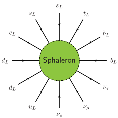
Figure 1: One of the 12-fermion processes which are in thermal equilibrium in the high-temperature phase of the standard model.

When the standard model particles form a heat bath of temperature $T$ the situation changes. At high temperatures, $T\geq T_{EW}\sim 100\;$GeV, the Higgs VEV ‘evaporates’, leading to a restoration of the electroweak symmetry and the disappearance of the potential barriers separating the different vacua. $B$ and $L$ violating transitions are then no longer suppressed [11].

The rate at which these processes occur is related to the free energy of field configurations which carry topological charge. In the electroweak part of the SM these so-called sphaleron processes lead to an effective interaction of all left-handed fermions [7] (cf. Fig. 1),

$$O_{B+L}=\prod\limits_{i}\left(q_{Li}q_{Li}q_{Li}l_{Li}\right)\,,$$ (3)

which indeed violates both baryon and lepton number by three units but conserves the combination $B-L$, in accord with Eq. (2).

The sphaleron transition rate in the symmetric phase of the SM has been evaluated by combining an analytical resummation with numerical lattice techniques [12]. The result is that sphaleron processes are in thermal equilibrium for temperatures in the range

$$100\,{\rm GeV}\lesssim T\lesssim 10^{12}\,{\rm GeV}\;.$$ (4)

These processes have a profound effect on the generation of the cosmological baryon asymmetry. Eq. (2) suggests that any $B+L$ asymmetry generated at temperatures $T>T_{EW}$, will be washed out. However, since only left-handed fields couple to sphalerons, a non-zero value of $B+L$ can persist in the high-temperature, symmetric phase if there exists a non-vanishing $B-L$ asymmetry. An analysis of the chemical potentials of all particle species in the high-temperature phase yields the following relation between the baryon asymmetry $\eta_{B}$ and the corresponding $L$ and $B-L$ asymmetries $\eta_{L}$ and $\eta_{B-L}$, respectively [14],

$$\eta_{B}\ =\ a_{sph}\ \eta_{B-L}\ =\ {a_{sph}\over a_{sph}-1}\ \eta_{L}\;.$$ (5)

Here $a_{sph}$ is a number ${\cal O}(1)$. In the SM with three generations and one Higgs doublet one has $a_{sph}=28/79$.

3 Leptogenesis

3.1 A qualitative overview

The deep connection between baryon and lepton number in the early universe has led to the realization that lepton number violating processes, whose presence is predicted by the seesaw model for light neutrino masses [4, 5], can be responsible for the observed cosmological baryon asymmetry.

In the seesaw model the smallness of light neutrino masses is explained through the mixing of left-handed neutrinos with right-handed neutrinos $\nu_{R}$ which are not present in the SM but are predicted in certain models of grand unification. The interactions of the SM are supplemented by the following Yukawa couplings of neutrinos,

$${\cal L}_{Y}=\overline{l_{L}}\,h\,\nu_{R}\,\phi+\overline{\nu_{R}^{c}}\,M\,\nu_{R}+{\rm h.c.}\;,$$ (6)

where $M$ is the Majorana mass matrix of the right-handed neutrinos, and the Yukawa couplings $h$ yield the Dirac neutrino mass matrix $m_{D}=hv$ after spontaneous breaking of the electroweak symmetry. Since the Majorana mass matrix $M$ is independent of electroweak symmetry breaking, one can have $M\gg m_{D}$, which leads to the mass eigenstates

$$\nu\simeq\nu_{L}+\nu_{L}^{c}=\nu^{c}\;,\quad N\simeq\nu_{R}+\nu_{R}^{c}=N^{c}\;,$$ (7)

with heavy neutrino masses $M$ and the light neutrino masses

$$m_{\nu}=-m_{D}{1\over M}m_{D}^{T}\;.$$ (8)

The heavy neutrinos are unstable and decay through their Yukawa couplings into SM lepton and Higgs doublets. Due to their Majorana nature, the heavy neutrinos $N$ can decay both into leptons and anti-leptons, i.e. lepton number is violated in these decays. In conjunction with $B+L$ violating sphaleron transitions this leads to the required non-conservation of baryon number. Further, violation of $C$ and $C\!P$ comes about since the Yukawa couplings $h$ are, in general, complex, thereby making possible the generation of a non-vanishing baryon asymmetry in these decays.

A further complication is that the heavy neutrinos also mediate lepton number violating scattering processes which can erase any lepton asymmetry [15, 14]. However, the interaction rates for these processes are suppressed by the large mass of the heavy neutrinos if the temperature $T$ is smaller than their mass. Hence, the lepton asymmetries produced in decays of the heavier neutrinos $N_{2,3}$ will be erased by lepton number violating scatterings mediated by the lightest of the heavy neutrinos, $N_{1}$. Therefore, in the simplest case of hierarchical heavy neutrino masses, $M_{1}\ll M_{2,3}$, only decays of $N_{1}$ can potentially explain the observed baryon asymmetry.

The required deviation from thermal equilibrium is provided by the expansion of the universe. When the universe has cooled down to a temperature of order the heavy neutrino mass $M_{1}$, the equilibrium number density becomes exponentially suppressed. If the neutrinos are sufficiently weakly coupled they are not able to follow the rapid change of the equilibrium particle distribution once the temperature falls below their mass. Hence, the deviation from thermal equilibrium consists in a too large number density of heavy neutrinos compared to the equilibrium density [16]. Technically this requires the total decay width of $N_{1}$ to be smaller than the expansion rate, the Hubble parameter $H$, at the time of decay, i.e. when $T\sim M_{1}$. This is the case if the effective neutrino mass, defined as

$$\widetilde{m}_{1}={(m_{D}^{\dagger}m_{D})_{11}\over M_{1}}\;,$$ (9)

is smaller than the equilibrium neutrino mass

$$m_{*}={16\pi^{5/2}\over 3\sqrt{5}}g_{*}^{1/2}{v^{2}\over M_{\rm p}}\simeq 10^{-3}~{}\mbox{eV}\;,$$ (10)

where we have used $M_{\rm p}=1.2\times 10^{19}$ GeV and $g_{*}=106.75$ as effective number of relativistic degrees of freedom in the plasma. The effective neutrino mass $\widetilde{m}_{1}$ is a measure of the strength of the coupling of $N_{1}$ to the thermal bath.

In order to see whether this mechanism of leptogenesis [6] can indeed explain the observed baryon asymmetry a careful numerical study is needed. As we shall see, successful leptogenesis is possible for $\widetilde{m}_{1}<m_{*}$ as well as $\widetilde{m}_{1}>m_{*}$. A quantitative description of this non-equilibrium process is obtained by means of kinetic equations.

3.2 Boltzmann equations

The evolution of particle number densities in the early universe is influenced not only by interactions but also by the expansion of the universe. It is convenient to scale out the expansion by considering the particle number $N_{X}$ in some comoving volume element instead of the number density $n_{X}$. For definiteness, we choose the comoving volume $R_{*}(t)^{3}$ which contains one photon at a time $t_{*}$ before the onset of leptogenesis,

$$N_{X}(t)=n_{X}(t)\,R_{*}(t)^{3}\;.$$ (11)

The final baryon asymmetry is expressed in terms of the baryon-to-photon ratio $\eta_{B}$, to be compared with the observed value $\eta_{B}^{\rm CMB}$ (cf. Eq. (1)). This is related to the $B-L$ asymmetry in a comoving volume element by

$$\eta_{B}={a_{sph}\over f}N_{B-L}^{\rm f},$$ (12)

where $f=2387/86$ is the dilution factor due to the production of photons from the onset of leptogenesis until recombination, assuming the standard isentropic expansion of the universe.

Further, it is convenient to replace time $t$ by $z=M_{1}/T$, where $M_{1}$ is the mass of the decaying neutrino. This is possible, since in a radiation dominated universe both variables are related by the expansion rate of the universe, the Hubble parameter $H$,

$$H=2t=\sqrt{4\pi^{3}g_{*}\over 45}\,{M_{1}^{2}\over M_{\rm p}}\,{1\over z^{2}}\;.$$ (13)

In the simplest case of a hierarchical mass spectrum of right-handed neutrinos, $M_{1}\ll M_{2,3}$, a numerical description of leptogenesis is provided by a set of two coupled differential equations [17, 18],

$${dN_{N_{1}}\over dz} = -(D+S)\,\left(N_{N_{1}}-N_{N_{1}}^{\rm eq}\right)\;,$$ (14)

$${dN_{B-L}\over dz} = -\varepsilon_{1}\,D\,\left(N_{N_{1}}-N_{N_{1}}^{\rm eq}\right)-W\,N_{B-L}\;,$$ (15)

where the terms on the right-hand side describe the effects of particle interactions. There are four classes of processes which contribute: decays, inverse decays, $\Delta L=1$ scatterings and $\Delta L=2$ processes mediated by heavy neutrinos. The term $D$ accounts for decays and inverse decays, while the scattering term $S$ represents the $\Delta L=1$ scatterings. Decays also yield the source term for the generation of the $B-L$ asymmetry, the first term in Eq. (15), while all other processes contribute to the total washout term $W$ which competes with the decay source term. Note that, in thermal equilibrium, $N_{N_{1}}=N_{N_{1}}^{\rm eq}$, no $B-L$ asymmetry can be generated, illustrating the need for a deviation from thermal equilibrium. The amount of $B-L$ asymmetry being produced by the source term is controlled by the $C\!P$ asymmetry $\varepsilon_{1}$ in the decay of $N_{1}$.

In order to understand the dependence of the solutions on the neutrino parameters, it is crucial to note that the interactions terms $D$ and $S$ as well as the contribution from $N_{1}$ exchange to $W$ are all proportional to the effective neutrino mass,

$$D,\;S,\;W_{1}\;\propto{M_{\rm p}\widetilde{m}_{1}\over v^{2}}\;,$$ (16)

whereas the strength of the remaining contribution to the washout term, $\Delta W$, is determined by $\overline{m}^{2}=m_{1}^{2}+m_{2}^{2}+m_{3}^{2}$, the sum over the light neutrino masses squared,

$$\Delta W\propto{M_{\rm p}M_{1}\overline{m}^{2}\over v^{4}}\;.$$ (17)

If one assumes a vanishing initial $B-L$ asymmetry before the onset of leptogenesis, i.e. at $z\ll 1$, the solution for $N_{B-L}$ has the simple form

$$N_{B-L}(z)=-{3\over 4}\,\varepsilon_{1}\,\kappa(z;\widetilde{m}_{1},M_{1}\overline{m}^{2})\;,$$ (18)

where we have introduced the efficiency factor $\kappa$ [19] which does not depend on the $C\!P$ asymmetry $\varepsilon_{1}$ and parametrizes the effect of scattering and decay processes. It is given by the following integral expression:

$$\kappa(z)={4\over 3}\int\limits_{z_{i}}^{z}dz^{\prime}\,D\,\left(N_{N_{1}}-N_{N_{1}}^{\rm eq}\right)e^{-\int_{z^{\prime}}^{z}dz^{\prime\prime}\,W(z^{\prime\prime})}\;.$$ (19)

It is normalized in such a way that its final value $\kappa_{f}=\kappa(\infty)$ approaches one in the limit of thermal initial abundance of heavy neutrinos, $N_{N_{1}}(z\ll 1)=N_{N_{1}}^{\rm eq}=3/4$ and no washout, $W=0$.

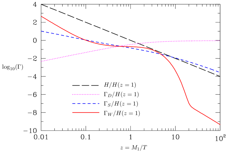
Figure 2: The expansion rate of the universe and the three interaction rates nomalized to the expansion rate at $z=1$ for a typical choice of parameters, $M_{1}=10^{10}\,$GeV, $\widetilde{m}_{1}=10^{-3}\,$eV and $\overline{m}=0.05\,$eV.

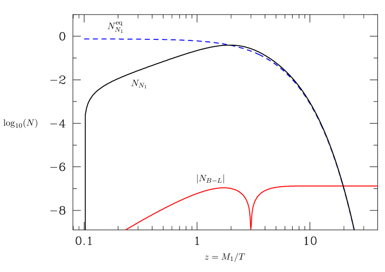
Figure 3: The evolution of the $N_{1}$ abundance and the $B-L$ asymmetry for the same choice of parameters as in Fig. 2 and $\varepsilon_{1}=10^{-6}$.

As an example, the three interaction rates, $(\Gamma_{D},\Gamma_{S},\Gamma_{W})=H\,z\,(D,S,W)$, and the Hubble parameter are shown in Fig. 2 for a typical choice of parameters, $M_{1}=10^{10}\,$GeV, $\widetilde{m}_{1}=10^{-3}\,$eV and $\overline{m}=0.05\,$eV. As can be seen from the figure, the out-of-equilibrium condition $\widetilde{m}_{1}\lesssim 10^{-3}\,$eV is fulfilled at $z=1$, i.e. all interaction rates are smaller than the Hubble parameter.

The corresponding evolution of the $N_{1}$ abundance and the $B-L$ asymmetry is shown in Fig. 3, starting at $z=0.1$ with a vanishing initial $N_{1}$ abundance. Although the neutrino production rates $\Gamma_{D}$ and $\Gamma_{S}$ are not in thermal equilibrium, they are still strong enough to produce a non-vanishing abundance of neutrinos at $z\lesssim 1$ and the equilibrium distribution is reached at $z\sim 2$. The required deviation from thermal equilibrium can clearly be seen as a small over-abundance of neutrinos for $z\gtrsim 2$. However, the decay rate $\Gamma_{D}$ also comes into thermal equilibrium at $z\sim 2$ leading to a rapid decay of the $N_{1}$ abundance and the production of a non-vanishing $B-L$ asymmetry. The change in sign in the asymmetry at $z\sim 3$ is due to the fact that the source term in eq. (15) changes sign once the $N_{1}$ abundance becomes larger than the equilibrium abundance, i.e. neutrino production processes at $z\lesssim 2$ lead to a ‘wrong sign’ asymmetry that partially cancels against the asymmetry produced in the $N_{1}$ decays at $z\gtrsim 2$.

4 CMB constraints on neutrino masses

We are now ready to discuss the implications of thermal leptogenesis for light and heavy neutrino masses. Combining Eqs. (12) and (18) one obtains

$$\eta_{B}=-d\,\,\varepsilon_{1}\,\kappa_{\rm f}(\widetilde{m}_{1},M_{1}\overline{m}^{2})\;,$$ (20)

where $d=3\,a_{\rm sph}/(4\,f)\simeq 10^{-2}$. Hence, determining the amount of baryon asymmetry produced in leptogenesis requires the calculation of both the final efficiency factor $\kappa_{\rm f}$ and the $C\!P$ asymmetry $\varepsilon_{1}$. A comparison with the observed value (cf. Eq. (1)) then allows to place stringent constraints on the involved seesaw parameters and, remarkably, on light and heavy neutrino masses.

4.1 Final efficiency factor

Starting from Eq. (19) and assuming a high initial temperature, $z_{i}=M_{1}/T_{\rm i}\ll 1$, the final efficiency factor can be calculated analytically [16, 20]. For values $M_{1}\,\overline{m}^{2}\ll 10^{14}\,{\rm GeV}\,[\overline{m}/(0.05\,{\rm eV})]^{2}$ the washout term $\Delta W$ can be neglected and the final efficiency factor depends only on the effective neutrino mass $\widetilde{m}_{1}$.

The results for the efficiency factor are summarized in Fig. 4. Two different regimes can clearly be distinguished. In the weak washout regime, $\widetilde{m}_{1}\ll 10^{-3}\,{\rm eV}$, the results strongly depend on the initial conditions and on theoretical assumptions, i.e. in that case predictions are strongly model dependent and affected by large theoretical uncertainties. On the other hand, in the strong washout regime, $\widetilde{m}_{1}\gg 10^{-3}\,{\rm eV}$, the dependence on the initial conditions is practically negligible and the theoretical uncertainties are small such that the final asymmetry can be predicted within $\sim 50\%$.

In both cases very precise analytical approximations for the final efficiency factor can be obtained. It is instructive to start with a simplified picture where the scattering term $S$ is neglected and only decays and inverse decays contribute. The decay parameter,

$$K\equiv{\Gamma_{D}(z=\infty)\over H(z=1)}={\widetilde{m}_{1}\over m_{*}}\,,$$ (21)

controls whether $N_{1}$ decays are in thermal equilibirium or not. Here $\Gamma_{D}(z=\infty)$ is the $N_{1}$ decay width and $m_{*}$ marks the boundary between the weak and strong washout regimes, as discussed in Section 3.1.

In the strong washout regime inverse decays rapidly thermalize the heavy neutrinos $N_{1}$ and the washout due to decays and inverse decays is strong enough to destroy an initial asymmetry that may have been present before the onset of leptogenesis [21], leading to a negligible dependence on initial conditions. Further, the integrand in Eq. (19) is peaked at a value $z_{B}\gg 1$, implying that the final asymmetry is produced around a well defined temperature of baryogenesis $T_{B}=M_{1}/z_{B}\ll M_{1}$, where the heavy neutrinos are fully non-relativistic. This contributes to reducing the theoretical uncertainties in the strong washout regime, since it has been shown that the Boltzmann equations employed here can be derived from a fully consistent quantum mechanical treatment in terms of Kadanoff-Baym equations in the non-relativistic limit [22].

In the strong washout regime the $N_{1}$ abundance closely tracks the equilibrium abundance and a simple expression for the final efficiency factor can be obtained,

$$\kappa_{f}(K)\simeq{2\over K\,z_{B}(K)}\,\left(1-e^{-{1\over 2}\,K\,z_{B}(K)}\right)\;.$$ (22)

Assuming thermal initial $N_{1}$ abundance, i.e. $N_{N_{1}}^{\rm i}=3/4$, this expression also reproduces the correct asymptotical limit in the weak washout regime, $K\ll 1$. In Fig. 4 this analytical result is represented by the short-dashed line which has to be compared to the numerical results, given by the solid lines.

In the weak washout regime the calculation is more involved if one starts from a vanishing initial $N_{1}$ abundance. Indeed, in this case the $N_{1}$ production by inverse decays leads to a negative contribution to the efficiency factor, corresponding to a ‘wrong-sign’ asymmetry, as discussed in Section 3.2. The final efficiency factor is thus the sum of a negative contribution, $\kappa^{-}_{\rm f}(K)$, and a positive one, $\kappa^{+}_{\rm f}(K)$. A very good approximation for these contributions that interpolates between the weak and strong washout regimes is given by

$$\kappa^{-}_{\rm f}(K) = -2\ e^{-{2\over 3}\,N(K)}\left(e^{{2\over 3}\overline{N}(K)}-1\right)\;,$$ (23)

$$\kappa^{+}_{\rm f}(K) = {2\over z_{B}(K)\,K}\left(1-e^{-{2\over 3}z_{B}(K)\,K\overline{N}(K)}\right)\;.$$ (24)

Here $N(K)\simeq(9\pi/16)K$ is the maximal $N_{1}$ number density being produced in the weak washout regime and $\overline{N}(K)$ interpolates between $N(K)$ and the maximal number density $N_{\rm eq}=3/4$ in the strong washout regime. For large $K$ the negative contribution is suppressed, while the positive one asymptotically approaches Eq. (22). On the other hand, in the weak washout regime the positive and negative contributions cancel each other to leading order in $K$, i.e. the total efficiency factor is of order $K^{2}$ [23], as shown in Fig. 4, where the short-dashed line again corresponds to the analytical solution and the solid one to the numerical integration of the Boltzmann equations.

This cancellation of the leading order contributions to the final efficiency factor in the weak washout regime no longer occurs when the scattering term $S$ is taken into account. Indeed, these scattering processes enhance the $N_{1}$ production thereby giving rise to an additional positive contribution to the efficiency factor. On the other hand, these scatterings are $C\!P$-conserving, i.e. they do not contribute to the negative part of the efficiency factor, as long as the contribution of $\Delta L=1$ scatterings to the washout term is negligible which is always the case in the weak washout regime. In this way scatterings can greatly enhance the final efficiency factor in the weak washout regime [24]. The drawback is that the result is very sensitive to different approximations being used in the computation of the scattering rates and different results, ranging from the case where scatterings are negligible to a behaviour $\kappa_{\rm f}\propto K$, have been obtained. Potentially important effects that have recently been discussed but are presently controversial include scattering processes involving gauge bosons [25, 26] and thermal corrections to the decay and scattering rates [27, 26]. The range of different results is represented in Fig. 4 by the hatched region. An additional uncertainty in the weak washout regime comes about due to the dependence of the final results on the initial $N_{1}$ abundance and a possible initial asymmetry created before the onset of leptogenesis.

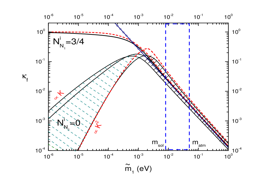
Figure 4: Final efficiency factor when the washout term $\Delta W$ is neglected.

The situation is very different in the strong washout regime. The final efficiency factor is not sensitive to the neutrino production since a thermal neutrino distribution is always reached at high temperatures, $z\ll 1$. However, $\Delta L=1$ scatterings also contribute to the washout term but their effect is small and thus the theoretical uncertainty arising from these scattering processes is not larger than about $50\%$. This uncertainty for values $\widetilde{m}_{1}>m_{*}\simeq 10^{-3}\,{\rm eV}$ is again indicated by the hatched region in Fig. 4. A much more important source of uncertainties are spectator processes [28], which can change the produced asymmetry by a factor of order one.

In the strong washout regime the highest efficiency is reached when scatterings are neglected and only decays and inverse decays are taken into consideration, which approximately corresponds to the results obtained in [26]. In this parameter range the final efficiency factor is given, within theoretical uncertainties, by the simple power law [20]

$$\kappa_{\rm f}=(2\pm 1)\,10^{-2}\,\left({0.01\,{\rm eV}\over\widetilde{m}_{1}}\right)^{1.1\pm 0.1}\;.$$ (25)

The only model independent information we have on $\widetilde{m}_{1}$ is that it has to be larger than the smallest neutrino mass $m_{1}$ [29]. However, a situation where $m_{1}<\widetilde{m}_{1}\ll m_{\rm sol}$ is rather artificial within neutrino mass models and the leptogenesis predictions are then very model dependent in the weak washout regime. In typical neutrino mass models values of $\widetilde{m}_{1}$ are usually in the mass range suggested by neutrino oscillations. It is remarkable that both the scale of solar neutrino oscillations, $m_{\rm sol}\equiv\sqrt{\Delta m^{2}_{\rm sol}}\simeq 8\times 10^{-3}\,{\rm eV}$, and the scale of atmospheric neutrino oscillations, $m_{\rm atm}\equiv\sqrt{\Delta m^{2}_{\rm atm}}\simeq 0.05\,{\rm eV}$, are much larger than the equilibrium neutrino mass $m_{*}$. Hence, the parameter range suggested by neutrino oscillations, $m_{\rm sol}\lesssim\widetilde{m}_{1}\lesssim m_{\rm atm}$, lies entirely in the strong washout regime where theoretical uncertainties are small and the efficiency factor is still large enough to allow for successful leptogenesis.

4.2 CP asymmetry

The $C\!P$ asymmetry $\varepsilon_{1}$ is the second crucial ingredient needed to calculate the baryon asymmetry. To leading order in the Yukawa coupling $h$, the $C\!P$ asymmetry is determined by the interference between tree level and vertex plus self-energy one-loop diagrams [30, 31] and can be consistently extracted from the $l\phi\rightarrow l\phi$ scattering processes [32].

We will be interested in the maximal $C\!P$ asymmetry for given neutrino masses. Assuming a hierarchy of the heavy neutrinos, $M_{2,3}\gg M_{1}$, $\varepsilon_{1}^{\rm max}$ depends on $M_{1}$, $\widetilde{m}_{1}$, $m_{1}$ and $m_{3}$ [21]. It can be expressed as

$$\varepsilon_{1}^{\rm max}(M_{1},\widetilde{m}_{1},m_{1},m_{3})=\varepsilon_{1}^{\rm max}(M_{1})\,\beta(\widetilde{m}_{1},m_{1},m_{3})\;,\quad\beta\leq 1\;.$$ (26)

The maximal asymmetry, i.e. $\beta=1$, is reached for $m_{1}=0$ and, with $m_{3}=\sqrt{m^{2}_{\rm atm}+m_{1}^{2}}$, it is given by [33]

$$\varepsilon_{1}^{\rm max}(M_{1})={3\over 16\pi}\,{M_{1}\,m_{\rm atm}\over v^{2}}\simeq 10^{-6}\,\left({M_{1}\over 10^{10}\,{\rm GeV}}\right)\,\left({m_{\rm atm}\over 0.05\,{\rm eV}}\right)\;.$$ (27)

An improved bound is obtained in the limit $m_{1}/\widetilde{m}_{1}\rightarrow 0$, where one obtains [34],

$$\beta(m_{1})={m_{3}-m_{1}\over m_{\rm atm}}\;.$$ (28)

Also important is the case of quasi-degenerate neutrinos, $m_{3}\simeq m_{1}$. In this region one finds [35, 36],

$$\beta(\widetilde{m}_{1},m_{1})\simeq{m_{3}-m_{1}\over m_{\rm atm}}\,\sqrt{1-{m_{1}^{2}\over\widetilde{m}_{1}^{2}}}\;.$$ (29)

For all neutrino mass models with moderately hierarchical heavy neutrinos, such that Eq. (26) applies, the observed baryon asymmetry yields constraints on the three neutrino parameters $\widetilde{m}_{1},m_{1}$ and $M_{1}$. In the following two sections we follow mostly the discussion in Ref. [20].

4.3 Lower bounds on heavy neutrino masses and reheating temperature

The maximal baryon asymmetry $\eta_{B}^{\rm max}(M_{1},\widetilde{m}_{1},m_{1})$ is the asymmetry corresponding to $\varepsilon_{1}^{\rm max}(M_{1},\widetilde{m}_{1},m_{1})$. The CMB bound then amounts to the requirement

$$\eta_{B}^{\rm max}(M_{1},\widetilde{m}_{1},m_{1})\geq\eta_{B}^{CMB}\;.$$ (30)

This represents an interesting constraint on the space of the three parameters $M_{1}$, $m_{1}$ and $\widetilde{m}_{1}$. We have seen that the absolute maximum of the $C\!P$ asymmetry is obtained for $m_{1}=0$. For $m_{1}\neq 0$ the function $\beta$ suppresses the $C\!P$ asymmetry [34]. Furthermore, the $\Delta L=2$ washout term becomes stronger when the absolute neutrino mass scale increases (cf. (17)). Therefore, the maximal baryon asymmetry $\eta_{B}^{\rm max}(M_{1},\widetilde{m}_{1},m_{1})$ is maximized for $m_{1}=0$, and in this case the allowed region in the space of the parameters $M_{1}$ and $\widetilde{m}_{1}$ is maximal [18].

In this way one finds an important lower bound on the value of $M_{1}$ [34, 18], by inserting the expression (27) into the CMB constraint (30) (cf. (20)),

$$M_{1}\geq M_{1}^{\rm min} = {1\over d}\,{16\,\pi\over 3}\,{v^{2}\over m_{\rm atm}}\,{\eta_{B}^{CMB}\over\kappa_{\rm f}}$$ (31)

$$\simeq 6.4\times 10^{8}\,{\rm GeV}\left(\eta_{B}^{CMB}\over 6\times 10^{-10}\right)\left(0.05\,{\rm eV}\over m_{\rm atm}\right)\,\kappa_{\rm f}^{-1}\;.$$

For thermal initial abundance, and in the limit $\widetilde{m}_{1}/m_{*}\rightarrow 0$, one has by definition $\kappa_{f}=1$, and therefore

$$M_{1}\geq(6.6\pm 0.8)\times 10^{8}\,{\rm GeV}\gtrsim 4\times 10^{8}\,{\rm GeV}\,.$$ (32)

Here the last inequality is the $3\,\sigma$ bound, with the experimental value of Eq. (1) for $\eta_{B}^{CMB}$, and $m_{\rm atm}=(0.051\pm 0.004)\,{\rm eV}$. In the case of a dynamically generated $N_{1}$ abundance the maximal efficiency factor is $\kappa_{\rm f}\simeq 0.18$, which yields the more stringent bound

$$M_{1}\,\geq\,(3.6\pm 0.4)\times 10^{9}\,{\rm GeV}\,\gtrsim\,2\times 10^{9}\,{\rm GeV}\;.$$ (33)

The most interesting case corresponds to the range $m_{\rm sol}\lesssim\widetilde{m}_{1}\lesssim m_{\rm atm}$, for which the power law Eq. (25) for $\kappa_{\rm f}$ can be used. Using the central value of $\kappa_{f}$ and neglecting the theoretical uncertainty, one obtains

$$M_{1}\gtrsim(3.3\pm 0.4)\times 10^{10}\,{\rm GeV}\,\left(\widetilde{m}_{1}\over 10^{-2}\,{\rm eV}\right)^{1.1}\;,$$ (34)

which yields the $3\,\sigma$ bound

$$M_{1}\gtrsim(1.5-10)\times 10^{10}\,{\rm GeV}\;.$$ (35)

The lower bound on $M_{1}$ is particularly interesting since it can be translated into a lower bound on the initial temperature $T_{\rm i}$ which, within inflationary models, corresponds to the reheating temperature.

So far we have assumed that the temperature $T_{\rm i}$ is larger than $M_{1}$. If one relaxes this assumption, the final efficiency factor is in general reduced. For small $\widetilde{m}_{1}$, however, the threshold value for $T_{\rm i}$, below which the reduction is appreciable, is given by $M_{1}$ itself. Below this temperature the $N_{1}$ abundance is either Boltzmann suppressed, for thermal initial abundance, or the $N_{1}$ production is considerably suppressed, for zero initial abundance. Therefore, for values $\widetilde{m}_{1}\lesssim 10^{-3}\,{\rm eV}$, the bounds (32) and (33) apply also to the reheating temperature $T_{\rm i}$.

In the more interesting case of strong washout, about $90\%$ of the final baryon asymmetry is produced in a temperature interval $z_{B}-2\lesssim z\lesssim z_{B}+2$. Hence the reheating temperature can be about $(z_{B}-2)$ times lower than $M_{1}$ without any appreciable change in the predicted final asymmetry [20]. In the interesting range $m_{\rm sol}\lesssim\widetilde{m}_{1}\lesssim m_{\rm atm}$ one has $z_{B}\simeq 6-8$, and therefore the bound Eq. (35) gets relaxed by a factor $4-6$, such that

$$T_{\rm i}\gtrsim(4\times 10^{9}-2\times 10^{10})\,{\rm GeV}\,.$$ (36)

Compared to the small $\widetilde{m}_{1}$ range, $\widetilde{m}_{1}\lesssim 10^{-3}$ eV, the lower bound on the reheating temperature is slightly more restrictive in the favoured range $m_{\rm sol}\lesssim\widetilde{m}_{1}\lesssim m_{\rm atm}$ due to the loss in efficiency.

4.4 Upper bound on light neutrino masses

For large values of the absolute neutrino mass scale the $\Delta W$ washout term cannot be neglected. The final efficiency factor can be calculated using the approximation that $\Delta W$ starts to be effective for $z>z_{B}$, where the asymmetry generation from decays has already terminated. This works very well in the strong washout regime. Since $\widetilde{m}_{1}\geq m_{1}$, this does not introduce any restriction if $m_{1}\gtrsim m_{*}\simeq 10^{-3}\,{\rm eV}$. One then has

$$\kappa_{\rm f}(\widetilde{m}_{1},\,M_{1}\overline{m}^{2})\simeq\kappa_{\rm f}(\widetilde{m}_{1})\,e^{-{\omega\over z_{B}}\,\left({M_{1}\over 10^{10}\,{\rm GeV}}\right)\,\left({\overline{m}\over{\rm eV}}\right)^{2}}\,,$$ (37)

where $\omega\simeq 0.186$ and $\kappa_{f}(\widetilde{m}_{1})$ is the efficiency factor calculated in the regime of small neutrino masses, neglecting the $\Delta W$ term. Because of the assumption of strong washout one can use the simple power law Eq. (25). At certain peak values of $M_{1}$ and $\widetilde{m}_{1}$ the maximal baryon asymmetry $\eta_{B}^{\rm max}$ reaches the absolute maximum

$${\eta_{B}^{\rm peak}(\overline{m})\over\eta_{B}^{CMB}}\propto{\chi\,m_{*}\,\xi\over\overline{m}^{4}}\;,$$ (38)

with $\chi\simeq 1.6\,{\rm eV}^{3}$ and $\xi\propto m_{\rm atm}^{2}$. This finally yields the leptogenesis bound on the neutrino masses, $m_{i}\lesssim 0.1\,$eV [21]. Deviations of the quantity $\xi$ from unity account for a change of the input parameters as well as various corrections, such as a possible enhancement of the $C\!P$ asymmetry or supersymmetry.

A more precise calculation has to take into account the dependence of neutrino masses on the renormalization scale. The running of the atmospheric neutrino mass scale $m_{\rm atm}$ from the Fermi scale $\mu=m_{Z}$ to the high scale $\mu\sim T_{B}$ makes the bound less restrictive. On the other hand the bound on $m_{i}$ obtained at high energies has to be evolved down to low energies. This second effect is dominant and thus taking the scale dependence into account makes the neutrino mass bound more restrictive [37]. The smallest effect is obtained for a Higgs mass $M_{h}\simeq 150\,{\rm GeV}$, which leads to a $\sim 20\%$ more restrictive bound [37]. Taking into account this effect one then obtains the $3\sigma$ bound [20]

$$m_{i}\lesssim 0.12\,{\rm eV}\,\xi^{1/4}\,.$$ (39)

Note, that the bound $m_{i}<0.1\,$eV conservatively accounts for the theoretical uncertainties including spectator processes [28] which make the bound more restrictive by about $0.02\,$eV . The strong suppression of the baryon asymmetry with increasing neutrino mass scale, $\eta_{B}\propto 1/\overline{m}^{4}$, which is reflected in the dependence $\xi^{1/4}$, makes the bound rather stable. This is different from the lower bounds on $M_{1}$ and $T_{i}$ which relax as $1/\xi$ [21].

It is important to keep in mind that the neutrino mass bound can be evaded, with some effort. A measurement of the neutrino mass scale above the leptogenesis bound would require significant modifications of the minimal leptogenesis scenario that we described. The possibilities include quasi-degenerate heavy neutrinos [21, 35], non-thermal leptogenesis scenarios [38, 39, 40] or a non-minimal seesaw mechanism as in theories with Higgs triplets [41, 42, 43].

4.5 Leptogenesis conspiracy

The upper bound on the neutrino masses (39) arises when the information on $m_{\rm atm}$ from neutrino mixing experiments is employed. The value of $m_{\rm atm}$ sets the scale for the transition from a hierarchical, with $m_{1}\ll m_{\rm atm}$, to a quasi-degenerate neutrino mass spectrum with $m_{1}\gtrsim m_{\rm atm}$. The joint action of the $C\!P$ asymmetry suppression for $m_{1}\gtrsim m_{\rm atm}$ and $\widetilde{m}_{1}\approx m_{1}$ (cf. (29)), together with the washout from the $\Delta W$ term, place a limit to the level of degeneracy of the light neutrino masses and, using the measured value of the atmospheric neutrino mass scale, an upper bound on the absolute neutrino mass scale.

We now want to study how this upper bound gets relaxed if the experimental measurement of the atmospheric neutrino mass scale is ignored. Since the maximal asymmetry is obtained for hierarchical neutrinos, i.e. $\beta=1$, we have to use the simple bound (27). This also implies that the upper bound on the absolute neutrino mass scale will coincide with an upper bound on the atmospheric neutrino mass scale itself, since $\overline{m}\simeq m_{\rm atm}\simeq m_{3}$. The maximal baryon asymmetry is then approximately given by

$$\eta_{B}^{\rm max}(M_{1},\widetilde{m}_{1},m_{3})=d\,\varepsilon_{1}^{\rm max}(M_{1})\,\kappa_{\rm f}(\widetilde{m}_{1},M_{1}\,m_{3}^{2})\;.$$ (40)

Using Eq. (37) it is easy to see that the maximum of the asymmetry is realized for

$$M_{1}\simeq 2\,z_{B}\,\,10^{13}\,{\rm GeV}\,\left({0.05\,{\rm eV}\over m_{3}}\right)^{2}\;,$$ (41)

and is then given by

$$\eta_{B}^{\rm max}(\widetilde{m}_{1},m_{3})\simeq 0.7\times 10^{-5}\,z_{B}(\widetilde{m}_{1})\,\kappa_{\rm f}(\widetilde{m}_{1})\,\left({0.05\,{\rm eV}\over m_{3}}\right)\,.$$ (42)

In the case of zero initial $N_{1}$ abundance the maximum is obtained for $\widetilde{m}_{1}\simeq 2\times 10^{-3}\,{\rm eV}$, where $k_{\rm f}\simeq 0.2$ and $z_{B}\simeq 2$ , implying

$$\eta_{B}^{\rm peak}(m_{3})\simeq 3\times 10^{-6}\,\left({0.05\,{\rm eV}\over m_{3}}\right)\,.$$ (43)

Note that the peak lies in the strong washout regime where results do not depend on the initial conditions.

For $m_{3}\simeq m_{\rm atm}\simeq 0.05\,{\rm eV}$, Eq. (43) is in good agreement with the numerical results of Ref. [18]. If we do not make use of the experimental information on $m_{\rm atm}$ and just require that the peak asymmetry is larger than the observed value given by Eq. (1), then we obtain the upper bound

$$m_{3}\lesssim 250\;{\rm eV}\;.$$ (44)

Together with Eq. (41) this implies the lower bound for heavy neutrinos masses,

$$M_{1}\gtrsim 2\times 10^{6}\;{\rm GeV}\;.$$ (45)

This exercise shows that without the experimental knowledge of $m_{\rm atm}$ the bound on light neutrino masses would have been much looser. However, it also demonstrates, even more remarkably, that the neutrino oscillation data, together with the laboratory bounds on light neutrino masses, represents a highly non trivial test of thermal leptogenesis.

As discussed in the previous section, the leptogenesis bound of 0.1 eV appears to have a theoretical uncertainty of about 0.03 eV. For comparison, ten years ago it was believed, based on the same equations, that Majorana masses $m_{3}\sim 10$ keV and $M_{1}\sim 1$ TeV were compatible with thermal leptogenesis [17]. During the past years theory and experiment contributed about equally, on a logarithmic scale, to the progress. On the theoretical side the better understanding of the Boltzmann equations was important whereas the measurement of the atmospheric neutrino mass scale was the crucial experimental ingredient.

Actually, the successful matching of thermal leptogenesis predictions with experimental data is even more intriguing. From Eq. (42) we can derive an upper bound on $\widetilde{m}_{1}$ by using the strong washout behaviour $\kappa_{\rm f}\simeq 2/(z_{B}\,K)$ (cf. (22)) and imposing the CMB bound, which yields, with $m_{\rm atm}=\sqrt{m_{3}^{2}-m_{1}^{2}}$,

$$\widetilde{m}_{1}\lesssim 20\,{\rm eV}\,\left({0.05\,{\rm eV}\over m_{\rm atm}}\right)\;,$$ (46)

again in very good agreement with the numerical results [18]. From this expression one reads off that only for $m_{\rm atm}\lesssim 1\,{\rm eV}$ it is possible to have $\widetilde{m}_{1}\sim m_{\rm atm}$. If the experiments had found $m_{\rm atm}\gg 1\,{\rm eV}$, thermal leptogenesis would have worked only for models with $\widetilde{m}_{1}\ll m_{\rm atm}$, requiring a large amount of fine tuning, as already pointed out. Furthermore, the favoured strong washout regime implies $m_{\rm atm}>m_{*}$. Hence, leptogenesis favours for the atmospheric mass scale the range $10^{-3}\,{\rm eV}-1\,{\rm eV}$, in remarkable agreement with experimental data. Thanks to this ‘conspiracy’ the seesaw mechanism, for the same values of the involved parameters, explains equally well both the neutrino masses and the observed baryon asymmetry, with a remarkable independence on the assumptions about the inflationary stage or, more generally, the cosmological stages that precede leptogenesis.

This conspiracy would become even more impressive if the lightest neutrino mass should turn out to be larger than $m_{*}$. This would imply, in a completely model independent way, $\widetilde{m}_{1}\gtrsim m_{*}$, with thermal leptogenesis in the strong washout regime. Together with the upper bound $m_{1}<0.1\,{\rm eV}$, this selects the optimal leptogenesis window $10^{-3}\,{\rm eV}\lesssim m_{1}\lesssim 0.1\,{\rm eV}$ for the absolute neutrino mass scale.

5 Flavour aspects

Leptogenesis is closely related to other processes involving neutrinos and charged leptons. The upper bound on the light neutrino masses and the lower bound on the heavy neutrino masses have already been discussed in the previous section. Very interesting are also the connection with neutrino mixing and with lepton flavour changing processes in supersymmetric theories. During the past years these subjects have been studied in great detail by many groups (cf. [44, 45, 46, 47, 48]). In the following we shall discuss two important examples, the possible connection between $C\!P$ violation in neutrino oscillations and leptogenesis, i.e. at low and high energies, and the relation between leptogenesis and the heavy neutrino mass spectrum.

In the standard model with right-handed neutrinos the masses and mixings of leptons are described by three complex matrices,

$${\cal L}_{M}=\overline{\nu_{L}}m_{D}\nu_{R}+\overline{e}_{L}m_{l}e_{R}\;+\overline{\nu_{R}^{c}}M\nu_{R}\;+\;h.c.\;.$$ (47)

For the Majorana mass matrix $M$ one expects $M\gg m_{D}$, which leads to three light and three heavy Majorana mass eigenstates, $\nu\simeq\nu_{L}+\nu_{L}^{c}=\nu^{c}$ and $N\simeq\nu_{R}+\nu_{R}^{c}=N^{c}$.

In the following we will work in a basis where $M$ is diagonal and real, with $M_{1}<M_{2}<M_{3}$, which is appropriate for leptogenesis. The light neutrino mass matrix $m_{\nu}$ and the charged lepton mass matrix $m_{l}$ are then diagonalized by the unitary transformations,

$$V^{(\nu)\dagger}m_{\nu}V^{(\nu)*} = -\left(\begin{array}[]{ccc}m_{1}&0&0\\ 0&m_{2}&0\\ 0&0&m_{3}\end{array}\right)\,=\,m_{\nu}^{\rm diag}\;,$$ (51)

$$V^{(e)\dagger}m_{e}\widetilde{V}^{(e)} = \left(\begin{array}[]{ccc}m_{e}&0&0\\ 0&m_{\mu}&0\\ 0&0&m_{\tau}\end{array}\right)\,=\,m_{l}^{\rm diag}\;.$$ (55)

The leptonic (MNS) mixing matrix

$$U=V^{(e)\dagger}V^{(\nu)}\;$$ (56)

describes the couplings of mass eigenstates in the charged current,

$${\cal L}^{(l)}_{EW}=-{g\over\sqrt{2}}\overline{e}_{L}\gamma^{\mu}U\nu_{L}\ W^{-}_{\mu}\ +\ldots\;,$$ (57)

which leads to neutrino oscillations.

It is well known that, in general, $C\!P$ violation in neutrino oscillations and in leptogenesis are unrelated [49]. The reason is that the $C\!P$ asymmetries $\varepsilon_{i}$ in heavy neutrino decays only depend on $m_{D}^{\dagger}m_{D}$. Hence, changing $m_{D}$ to $Km_{D}$, where $K$ is a general unitary matrix, leaves $\varepsilon_{i}$ invariant whereas the leptonic mixing matrix $U=V^{(e)\dagger}V^{(\nu)}$ is changed to $U=V^{(e)\dagger}KV^{(\nu)}$, and therefore arbitrary. Still, the question remains whether in some physically well motivated cases a connection between $C\!P$ violation at low and high energies exists.

$C\!P$ violating observables are most conveniently described by weak basis invariants which are inert under a unitary transformation, $l\rightarrow Kl$, of the lepton doublet $l=(\nu_{L},e_{L})$. For neutrino oscillations the appropriate variable is the commutator between the hermitian matrices $H_{\nu}=m_{\nu}m_{\nu}^{\dagger}$ and $H_{l}=m_{l}m_{l}^{\dagger}$ [50, 51],

$${\rm Tr}[H_{\nu},H_{l}]^{3}\,\propto\,\Delta_{\nu 21}\Delta_{\nu 32}\Delta_{\nu 31}\Delta_{l21}\Delta_{l32}\Delta_{l31}\,J_{l}\;,$$ (58)

$$\qquad\Delta_{\nu 21}=m_{2}^{2}-m_{1}^{2}\,,\ldots,\Delta_{l21}=m_{\mu}^{2}-m_{e}^{2}\,,\ldots\;,$$ (59)

where $J_{l}$ is the leptonic Jarlskog invariant [52],

$$J_{l}\,=\,\rm{Im}[U_{11}U_{22}U_{12}^{*}U_{21}^{*}]\,\propto\,\sin{\delta}\;,$$ (60)

which is proportional to the $C\!P$ violating phase $\delta$ of the mixing matrix $U$. In a basis where the charged lepton matrix $m_{l}$ is diagonal and real one has

$${\rm Tr}[H_{\nu},H_{l}]^{3}\,\propto\,\Delta_{l21}\Delta_{l32}\Delta_{l31}\,{\rm Im}[H_{\nu 12}H_{\nu 23}H_{\nu 31}]\;;$$ (61)

correspondingly, for diagonal and real $m_{\nu}$ one has

$${\rm Tr}[H_{\nu},H_{l}]^{3}\,\propto\,\Delta_{\nu 21}\Delta_{\nu 32}\Delta_{\nu 31}\,{\rm Im}[H_{l12}H_{l23}H_{l31}]\;.$$ (62)

The $C\!P$ asymmetry in $N_{1}$ decays can be conveniently expressed in terms of the weak basis invariant [22]

$$\varepsilon_{1}\propto{\rm Im}[m_{D}^{\dagger}m_{\nu}m_{D}^{*}]_{11}\;.$$ (63)

Comparing Eqs. (62) and (63) the independence of $C\!P$ violation at low and high energies is obvious. In a basis where $m_{\nu}$ is diagonal and real, $C\!P$ violation in neutrino oscillations is entirely determined by the phases $m_{l}$ whereas the lepton asymmetry only depends on the phases of $m_{D}$.

An interesting example is the case of only two heavy Majorana neutrinos, $N_{1}$ and $N_{2}$, which corresponds to the limit where $N_{3}$ decouples [53]. For a given texture of $m_{D}$ one then obtains (cf. (61), (63)),

$$\varepsilon_{1}\propto{\rm Im}[H_{\nu 12}H_{\nu 23}H_{\nu 31}]\propto\sin{\delta}\;.$$ (64)

Hence both, the $C\!P$ violation at low and at high energies, are determined by the Dirac phase $\delta$. A further low energy quantity is the Majorana phase entering neutrinoless double beta decay. In some models with maximal atmospheric neutrino mixing this phase coincides with the leptogenesis phase [54]. All $C\!P$ phases can also be related in models of spontaneous $C\!P$ violation [50, 55].

Another important question is the connection between leptogenesis and the heavy neutrino mass spectrum. In the lepton mass eigenstate basis the neutrino mass matrix can be reconstructed from data, i.e. the leptonic mixing matrix and the neutrino masses,

$$m_{\nu}=-U^{(\nu)}m_{\nu}^{\rm diag}U^{(\nu)T}\;.$$ (65)

The heavy neutrino mass matrix is then determined by $m_{\nu}$ and $m_{D}$,

$$M^{-1}=-m_{D}^{-1}m_{\nu}(m_{D}^{T})^{-1}\;.$$ (66)

Using the SO(10) mass relation $m_{D}=m_{u}$, where $m_{u}$ denotes the up-type quark mass matrix, and assuming that in the lepton mass eigenstate basis $m_{u}$ is also diagonal and real, $m_{u}={\rm diag}(m_{u},m_{c},m_{t})$, one obtains the heavy neutrino masses in terms of $m_{\nu}$, $m_{u}$, $m_{c}$ and $m_{t}$ [56]. Neglecting the hierarchy among the small neutrino masses one estimates that the hierarchy among the heavy neutrinos is very large,

$${M_{1}\over M_{3}}\sim\left({m_{u}\over m_{t}}\right)^{2}\sim 10^{-10}\;.$$ (67)

With $M_{3}\sim m_{t}^{2}/\sqrt{\Delta m^{2}_{\rm atm}}\sim 10^{15}$ GeV, this implies $M_{1}\sim 10^{5}$ GeV. A detailed study yields masses in the range $M_{1}\sim 10^{4}\ldots 10^{6}$ GeV. As we saw in the previous section, such small masses are incompatible with conventional thermal leptogenesis. A possible way out are quasi-degenerate heavy neutrino masses [56]. Alternatively, the most naive SO(10) mass relations are not correct.

Parameters consistent with thermal leptogenesis have recently been obtained in a six-dimensional SO(10) GUT model, compactified on an orbifold [57]. Due to mixings with a heavy lepton doublet and a heavy right-handed down-type quark one finds for the mass matrices in a particular flavour basis the relations,

$$M\propto m_{u}\;,\quad m^{\prime}_{D}\sim m^{\prime}_{d}\sim m^{\prime}_{e}\;.$$ (68)

Here $M$ and $m_{u}$ are diagonal $3\times 3$ matrices, and $m^{\prime}_{D}$, $m^{\prime}_{d}$ and $m^{\prime}_{e}$ are $4\times 4$ matrices, due to the mixing with the heavy states. Integrating them out, the neutrino mass matrix can be expressed approximately in terms of the quark mass matrices,

$$m_{\nu}\propto m_{d}{1\over m_{u}}m_{d}^{T}\;.$$ (69)

For the light neutrino masses this leads to the estimate

$${m_{1}\over m_{3}}\sim\left({m_{d}\over m_{b}}\right)^{2}{m_{t}\over m_{b}}\sim 0.1\;.$$ (70)

A detailed calculation [57] confirms this result. Furthermore, one finds the mixing angle $\Theta_{13}\sim(m_{c}m_{b})/(m_{t}m_{s})\sim 0.1$, and $\varepsilon\sim 10^{-6}$, $\widetilde{m}_{1}\sim 10^{-2}$ eV, $M_{1}\sim(m_{u}/m_{t})M_{3}\sim 10^{10}$ GeV, consistent with thermal leptogenesis.

6 Cosmological aspects

It is well known that the temperature required by thermal leptogenesis, $T_{B}\gtrsim 10^{9}$ GeV, is potentially in conflict with the thermal production of gravitinos in the early universe [58, 59]. Late gravitino decays after nucleosynthesis significantly alter the successful BBN predictions.

The production of gravitinos is dominated by QCD processes, and the gravitino number density increases linearly with the reheating temperature after inflation,

$${n_{3/2}\over n_{\gamma}}\propto{g_{3}^{2}\over M_{\rm p}^{2}}\,T_{R}\;,$$ (71)

where $g_{3}$ is the QCD gauge coupling. Correspondingly, the BBN upper bound on the allowed gravitino energy density, $\rho_{3/2}=m_{3/2}n_{3/2}$, implies an upper bound on the reheating temperature. Detailed studies [60, 61] lead to the stringent bounds $T_{R}<10^{7}-10^{9}$ GeV for gravitino masses in the range $m_{3/2}=0.1-1$ TeV. Hence, unstable gravitinos are in conflict with thermal leptogenesis, unless the gravitino mass is very large, $m_{3/2}\gtrsim 50$ TeV.

Non-thermal leptogenesis models are still compatible with the above bounds on the reheating temperature. For instance, in some supersymmetric models the scalar partner $\widetilde{N}_{1}$ of the heavy neutrino $N_{1}$ might be the inflaton [62] and its decays could then generate the baryon asymmetry. In this case the leptogenesis temperature can be below $10^{7}$ GeV [63, 26], which would be consistent with the above gravitino bounds on $T_{R}$. However, a recent analysis of the BBN constraints [64] with particular attention to the hadronic decay modes of the gravitino yields the much stronger bound $T_{R}\ll 10^{6}$ GeV for gravitino masses $m_{3/2}=0.1-1$ TeV. Hence, unless the gravitino is extremely heavy, also non-thermal leptogenesis appears to be inconsistent with unstable gravitinos.

Already in connection with thermal leptogenesis, it has therefore been suggested that the gravitino may be the lightest superparticle (LSP) and stable [65]. In this case, gravitino production is enhanced [66],

$${n_{3/2}\over n_{\gamma}}\propto{g_{3}^{2}\over M_{\rm p}^{2}}\,\left({m_{\widetilde{g}}\over m_{3/2}}\right)^{2}\,T_{R}\;,$$ (72)

where $m_{\widetilde{g}}$ is the gluino mass. Consistency with BBN and the observed amount of dark matter then yields an upper bound on the gravitino mass and a lower bound on the mass of the next-to-lightest superparticle (NSP). In [65] the case of a higgsino NSP was analyzed, which is now disfavoured due to the improved BBN bounds on hadronic NSP decays [64]. Still viable is the case where a scalar lepton is the NSP [67]. For $T_{B}=3\times 10^{9}$ GeV the upper bound on the gluino mass is $m_{\widetilde{g}}<1.3$ TeV if a scalar tau is the NSP; for a scalar neutrino NSP one finds $m_{\widetilde{g}}<1.8$ TeV [67].

The relic density of gravitinos is determined by thermal production at the reheating temperature $T_{R}$ after inflation and also by NSP decays after their freeze-out temperature. It is an interesting possibility that the latter process dominates. This would be the case for low reheating temperatures, incompatible with leptogenesis. One then obtains a prediction for the amount of gravitino dark matter which is independent of the reheating temperature [68]. If gravitinos are the only component of dark matter, the superparticles have to be rather heavy. For $\widetilde{\tau}_{R}$ as NSP one finds $m_{3/2}=0.2-1$ TeV and $m_{\widetilde{\tau}_{R}}\geq 0.5$ TeV [69].

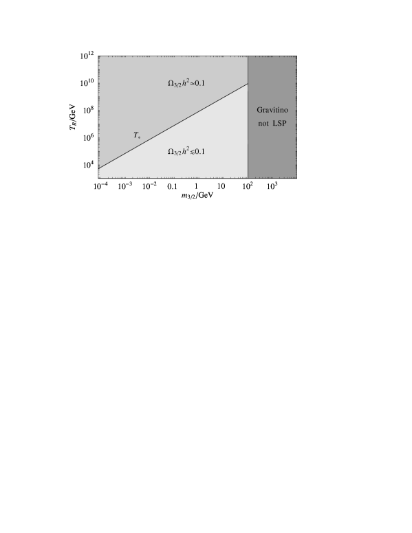
Figure 5: Relic gravitino density for different values of reheating temperature and gravitino mass. $\xi/\eta^{2}=1$. $m_{\widetilde{g}}=1$ TeV, which implies $m_{3/2}<0.1$ TeV for a stable gravitino. For $T_{R}>T_{*}$, $\Omega_{3/2}h^{2}$ is independent of $T_{R}$ and $m_{3/2}$.

Recently, it has been pointed out that the thermal production of gravitinos is significantly changed in theories where the gauge coupling depends on the expectation value of a scalar field $\phi$ [70]. For instance, in the case of gaugino mediation one has,

$${1\over g_{0}^{2}}+{\phi_{T}\over M}={1\over g^{2}(\phi_{T})}\;,$$ (73)

where $g_{0}$ is the zero-temperature gauge coupling, $M$ is a mass scale between the unification scale and the Planck mass, and $\phi_{T}$ is the deviation of the field $\phi$ from its zero-temperature value at temperature $T$. At temperatures above a critical temperature,

$$T_{*}\sim m_{3/2}\left({M_{\rm p}\over m_{\widetilde{g}}}\right)^{1/2}\;,$$ (74)

the gauge couplings decreases, and the gravitino production is frozen. Remarkably, the relic gravitino density is essentially determined just by the gluino mass [70],

$$\Omega_{3/2}h^{2}\simeq(0.05-0.2)\times\left(\frac{m_{\widetilde{g}}}{1~{}{\rm TeV}}\right)^{3/2}\left(\frac{\xi}{\eta^{2}}\right)^{1/4}\;,$$ (75)

where the factor $\xi/\eta^{2}$ depends on the mechanism of supersymmetry breaking. For gaugino and gravity mediation one has $\xi/\eta^{2}={\cal O}(1)$. The observed amount of dark matter is then obtained for a gluino mass $m_{\widetilde{g}}\sim 1$ TeV, which will be tested at the LHC. As Fig. 5 illustrates, the temperature where thermal leptogenesis takes place is likely to be larger than the critical temperature $T_{*}$. For a gluino mass $m_{\widetilde{g}}\sim 1$ TeV one then obtains automatically the observed amount of cold dark matter.

Finally, thermal leptogenesis can also be consistent with gravitino dark matter if the gravitino is very light, $m_{3/2}\simeq 0.1-10$ MeV [71, 72], which is realized in gauge mediation models. Alternatively, the gravitino can also be very heavy, $m_{3/2}\sim 100$ TeV [73, 74], as in anomaly mediation.

In summary, leptogenesis strongly constrains the nature of dark matter. For very heavy unstable gravitinos, $m_{3/2}\sim 100$ TeV, where ordinary WIMPs can be the dark matter, the superparticle mass spectrum is strongly restricted. Alternatively, the gravitino has to be the LSP with a mass below $\sim 0.1$ TeV; the observed value of $\Omega_{CDM}h^{2}$ can then be naturally explained. Hence, the identification of the invisible dark matter, which will hopefully take place at colliders in the coming years, will also shed light on baryogenesis and therefore on the origin of the visible matter.

References

References

- [1] WMAP Collaboration, D. N. Spergel et al., Astrophys. J. Suppl. 148 (2003) 175
- [2] M. Tegmark et al., Phys. Rev. D 69 (2004) 103501
- [3] A. D. Sakharov, JETP Lett. 5 (1967) 24
- [4] T. Yanagida, in Workshop on Unified Theories, KEK report 79-18 (1979) p. 95
- [5] M. Gell-Mann, P. Ramond, R. Slansky, in Supergravity (North Holland, Amsterdam, 1979) eds. P. van Nieuwenhuizen, D. Freedman, p. 315
- [6] M. Fukugita, T. Yanagida, Phys. Lett. B 174 (1986) 45
- [7] G. ’t Hooft, Phys. Rev. Lett. 37 (1976) 8
- [8] N. S. Manton, Phys. Rev. D 28 (1983) 2019
- [9] F. R. Klinkhammer, N. S. Manton, Phys. Rev. D 30 (1984) 2212
- [10] V. A. Rubakov, M. E. Shaposhnikov, Phys. Usp. 39 (1996) 461
- [11] V. A. Kuzmin, V. A. Rubakov, M. E. Shaposhnikov, Phys. Lett. B 155 (1985) 36
- [12] D. Bödeker, M. Laine, K. Rummukainen, Phys. Rev. D 61 (2000) 056003
- [13] S. Yu. Khlebnikov, M. E. Shaposhnikov, Nucl. Phys. B 308 (1988) 885
- [14] J. A. Harvey, M. S. Turner, Phys. Rev. D 42 (1990) 3344
- [15] M. Fukugita, T. Yanagida, Phys. Rev. D 42 (1990) 1285
- [16] E. W. Kolb, M. S. Turner, The Early Universe, (Addison-Wesley, New York, 1990)
- [17] M. A. Luty, Phys. Rev. D 45 (1992) 455
- [18] W. Buchmüller, P. Di Bari, M. Plümacher, Nucl. Phys. B 643 (2002) 367
- [19] R. Barbieri, P. Creminelli, A. Strumia, N. Tetradis, Nucl. Phys. B 575 (2000) 61
- [20] W. Buchmüller, P. Di Bari, M. Plümacher, hep-ph/0401240
- [21] W. Buchmüller, P. Di Bari, M. Plümacher, Nucl. Phys. B 665 (2003) 445
- [22] W. Buchmüller, S. Fredenhagen, Phys. Lett. B 483 (2000) 217
- [23] J. N. Fry, M. S. Turner, Phys. Rev. D 24 (1981) 3341
- [24] M. Plümacher, Z. Phys. C 74 (1997) 549
- [25] A. Pilaftsis and T. E. J. Underwood, hep-ph/0309342
- [26] G. F. Giudice, A. Notari, M. Raidal, A. Riotto and A. Strumia, Nucl. Phys. B 685 (2004) 89
- [27] L. Covi, N. Rius, E. Roulet, F. Vissani, Phys. Rev. D 57 (1998) 93
- [28] W. Buchmüller, M. Plümacher, Phys. Lett. B 511 (2001) 74
- [29] M. Fujii, K. Hamaguchi, T. Yanagida, Phys. Rev. D 65 (2002) 115012
- [30] M. Flanz, E. A. Paschos, U. Sarkar, Phys. Lett. B 345 (1995) 248; ibid. B 384 (1996) 487 (E)
- [31] L. Covi, E. Roulet, F. Vissani, Phys. Lett. B 384 (1996) 169
- [32] W. Buchmüller, M. Plümacher, Phys. Lett. B 431 (1998) 354
- [33] K. Hamaguchi, H. Murayama, T. Yanagida, Phys. Rev. D 65 (2002) 043512
- [34] S. Davidson, A. Ibarra, Phys. Lett. B 535 (2002) 25
- [35] T. Hambye, Y. Lin, A. Notari, M. Papucci, A. Strumia, hep-ph/0312203
- [36] P. Di Bari, Proceedings of the Second International Woorkshop on Neutrino Oscillations in Venice, ed. M. Baldo Ceolin, December 3-5, 2003
- [37] S. Antusch, J. Kersten, M. Lindner, M. Ratz, Nucl. Phys. B 674 (2003) 401
- [38] G. Lazarides, Q. Shafi, Phys. Lett. B 258 (1991) 305
- [39] H. Murayama, T. Yanagida, Phys. Lett. B 322 (1994) 349
- [40] G. F. Giudice, M. Peloso, A. Riotto, I. Tkachev, JHEP 9908 (1999) 014
- [41] T. Hambye and G. Senjanovic, Nucl. Phys. B 582 (2004) 73
- [42] W. Rodejohann, hep-ph/0403236
- [43] S. Antusch, S. F. King, hep-ph/0405093
- [44] I. Masina, hep-ph/0210125
- [45] Z.-Z. Xing, hep-ph/0307359
- [46] S. F. King, hep-ph/0310204
- [47] G. Altarelli, F. Feruglio, hep-ph/0405048
- [48] J. R. Ellis, hep-ph/0403247
- [49] W. Buchmüller, M. Plümacher, Phys. Lett. B 389 (1996) 73
- [50] G. C. Branco, T. Morozumi, B. M. Nobre, M. N. Rebelo, Nucl. Phys. B 617 (2001) 475
- [51] G. C. Branco, hep-ph/0309215
- [52] C. Jarlskog, Phys. Rev. Lett. 55 (1985) 1039
- [53] P. H. Frampton, S. L. Glashow, T. Yanagida, Phys. Lett. B 548 (2002) 119
- [54] W. Grimus, L. Lavoura, hep-ph/0311362
- [55] Y. Achiman, hep-ph/0403309
- [56] E. Kh. Akhmedov, M. Frigerio, A. Yu. Smirnov, JHEP 09 (2003) 021
- [57] T. Asaka, W. Buchmüller, L. Covi, Phys. Lett. B 563 (2003) 209
- [58] M. Yu. Khlopov, A. D. Linde, Phys. Lett. B 138 (1984) 265
- [59] J. Ellis, J. E. Kim, D. V. Nanopoulos, Phys. Lett. B 145 (1984) 181
- [60] M. Kawasaki, K. Kohri, T. Moroi, Phys. Rev. D 63 (2001) 103502
- [61] R. H. Cyburt, J. Ellis, B. D. Fields, K. A. Olive, Phys. Rev. D 67 (2003) 103521
- [62] H. Murayama, H. Suzuki, T. Yanagida, J. Yokoyama, Phys. Rev. Lett. 70 (1993) 1912
- [63] J. R. Ellis, M. Raidal, T. Yanagida, Phys. Lett. B 581 (2004) 9
- [64] M. Kawasaki, K. Kohri, T. Moroi, astro-ph/0402490
- [65] M. Bolz, W. Buchmüller, M. Plümacher, Phys. Lett. B 443 (1998) 209
- [66] T. Moroi, H. Murayama, M. Yamaguchi, Phys. Lett. B 303 (1993) 289
- [67] M. Fujii, M. Ibe, T. Yanagida, Phys. Lett. B 579 (2004) 6
- [68] J. L. Feng, A. Rajaraman, F. Takayama, Phys. Rev. Lett. 91 (2003) 011302-1
- [69] J. L. Feng, S. Su, F. Takayama, hep-ph/0404198
- [70] W. Buchmüller, K. Hamaguchi, M. Ratz, Phys. Lett. B 574 (2003) 156
- [71] M. Fujii, T. Yanagida, Phys. Lett. B 549 (2002) 273
- [72] M. Fujii, M. Ibe, T. Yanagida, Phys. Rev. D 69 (2004) 015006
- [73] M. A. Luty, R. Sundrum, Phys. Rev. D 67 (2003) 045007
- [74] M. Ibe, R. Kitano, H. Murayama, T. Yanagida, hep-ph/0403198