A Numerical Analysis of the Supersymmetric Flavor Problem and Radiative Fermion Masses

Abstract

We study the SUSY flavor problem in the MSSM, we are namely interested in estimating the size of the SUSY flavor problem and its dependence on the MSSM parameters. For that, we made a numerical analysis randomly generating the entries of the sfermion mass matrices and then determinated which percentage of the points are consistent with current bounds on the flavor violating transitions on lepton flavor violating (LFV) decays $l_{i}\rightarrow l_{j}\,\gamma$. We applied two methods, mass-insertion approximation method (MIAM) and full diagonalization method (FDM). Furthermore, we determined which fermion masses could be radiatively generated (through gaugino-sfermion loops) in a natural way, using those random sfermion matrices. In general, the electron mass generation can be done with 30% of points for large $\tan\beta$, in both schemes the muon mass can be generated by 40% of points only when the most precise sfermion splitting (from the FDM) is taken into account.

I Introduction.

Weak-scale supersymmetry (SUSY) review , has notably become one of the leading candidates for physics beyond the standard model, by supporting the mechanism of electroweak symmetry breaking (EWSB). Being a new fundamental space-time symmetry, SUSY necessarily extends the SM particle content by including superpartners for all fermions. Because the mass spectrum of the superpartners needs to be lifted, SUSY must be softly broken, this is needed so in order to maintain its ultraviolet properties. SUSY breaking is parameterized in the Minimal Supersymmetric SM (MSSM) by the soft-breaking lagrangian Chung:2003fi ; as an outcome, the combined effects of the large top quark Yukawa coupling and the soft-breaking masses, make radiatively inducing the breaking of the electroweak symmetry possible. The Higgs sector of the MSSM includes two Higgs doublets, perhaps being the light Higgs boson ($m_{h}\leq 125$ GeV) the strongest prediction of the model.

However, the soft breaking sector of the MSSM is often problematic with low-energy flavor changing neutral currents (FCNC) without making specific assumptions about its free parameters. Minimal choices to satisfy those constraints, such as assuming universality of squark masses, have been widely studied in literature Chung:2003fi . However, non-minimal flavor structures could be generated in a variety of contexts. For instance, within the context of realistic unification models by the evolution of soft-terms, from a high-energy GUT scale to the weak scale. Similarly, models that attempt to address the flavor problem, could induce sfermion soft-terms that reflect the underlying flavor symmetry of the fermion sector nondA ; Mura .

It is not a trivial task to find models of SUSY breaking that can actually generate minimal and safe patterns. This is the so called SUSY flavor problem. The known solutions include the following: degeneracy gabbiani (sfermions of different families have the same mass), proportionality gabbiani (trilinear terms are proportional to the Yukawa terms), decoupling Arkani-Hamed:1997ab (superpartners are too heavy to affect low energy physics) and alignment seiberg (the same physics that explains the pattern of fermion masses and mixing angles, forces the sfermion mass matrices to be aligned with the fermion ones, in a way that the fermion-sfermion-gaugino vertices remain close to diagonal).

Sometimes the SUSY flavor problem is stated by saying that if the sfermion mass matrix entries were randomly generated , most of these points would lead to the exclusion of the MSSM. In this paper, we would like to quantify the formerly statement, namely, we want to estimate the size of the SUSY flavor problem, and to determine its dependence on the parameters of the MSSM. Then, one would like to determine what would be left of the SUSY flavor problem after Tevatron and LHC will deliver bounds on the masses of the superpartners, or luckily a signal of their presence! Rather, we focus on lepton sector, we particularly use the LFV decays $l_{i}\rightarrow l_{j}+\gamma$ to make our point, namely to derive bounds on the parameters of the MSSM and to determine the viability and interplay of the solutions above.

First, we evaluate the LFV decays above using the mass-insertion approximation method (MIAM), both for muon and tau decays. Our procedure will consist first on writing the off-diagonal elements of the slepton mass matrices as the product of $O(1)$ coefficients times an average sfermion mass parameter, then we randomly generate $10^{5}$ points for the $O(1)$ coefficients, and determine which fraction of such points satisfies the current bounds on the LFV transitions. We repeat this procedure for different values of other relevant parameters of the MSSM, such as $\tan\beta$, gaugino masses, $\mu$-parameter and the sfermion mass scale.

Next, to estimate how much we can trust the MIAM, we compare those results with the ones coming from particular models that enable to obtain exact diagonalization for the sfermion mass matrices. Namely, we take into account that the constraints on sfermion mixing coming from low-energy data, mainly suppress the mixing between the first two family sleptons, but still allows large flavor-mixings between the second- and third-family sleptons, i.e. the smuon ($\tilde{\mu}$) and stau ($\tilde{\tau}$), which can be as large as $O(1)$ FCNC . Thus, we consider models where the mixing involving the selectrons could be neglected, as it involves small off-diagonal entries in the slepton mass matrices. But the $\tilde{\mu}-\tilde{\tau}$ mixing will involve large off-diagonal entries in the sfermion mass matrices, which requires at least a partial diagonalization in order to be treated in a consistent manner. Namely, in our models the general $6\times 6$ slepton-mass-matrix will include a $4\times 4$ sub-matrix involving only the $\tilde{\mu}-\tilde{\tau}$ sector, which can be exactly diagonalized , similarly to the squark case first discussed in Ref.oursqmix . Since we follow a bottom-up approach, we simply take an Ansatz for the $A$-terms valid at the TeV-scale; such large off-diagonal entries can be motivated by considering the large mixing detected with atmospheric neutrinos superkam , especially in the framework of GUT models with flavor symmetries. Then, we repeat the above method of random generation for the parameters of the sfermion matrices, which will then be diagonalized. Armed with the exact expressions for the mass and mixing matrices and the interaction lagrangian written in terms of mass eigenstates, we evaluate the fraction of points that satisfy all the LFV constraints coming from the $\tau\rightarrow\mu+\gamma$ decays. The results with exact diagonalization for LFV tau decays will be compared with those obtained using the MIAM .

Another aspect of the Flavor Problem involves the possibility to radiatively induce the fermion masses which are known to be possible within SUSY through sfermion-gaugino loops. Here, we shall determine which fraction of points can generate correctly the fermion masses through sfermion-gaugino loops. Again, we are interested in comparing the results obtained using FDM with those of the MIAM. Implications for LFV in the Higgs sector are discussed in Refs. Diaz-Cruz:2002er ; Diaz-Cruz:1999xe .

The organization of this paper goes as follows: in section II we discuss the SUSY flavor problem in the lepton sector, using the mass-insertion approximation. This section includes the evaluation of the radiative LFV loop transitions ($l_{i}\rightarrow l_{j}+\gamma$) with a random generation of the slepton $A$-terms. Then, in section III we present an Ansatz for soft breaking trilinear terms, the diagonalization of the resulting sfermion mass matrices, and we repeat the calculus of the previous section. The radiative generation of fermion masses is discussed in detail in section IV, within the context of the MSSM. Finally, our conclusions are presented in section V.

II The SUSY flavor problem in the Super CKM basis.

II.1 The slepton mass matrices in the MSSM

First, we discuss the slepton mass matrices and the gaugino-lepton-slepton interactions. The MSSM soft-breaking slepton sector contains the following quadratic mass-terms and trilinear $A$-terms:

$$\begin{array}[]{l}{\cal L}_{soft}=-{\widetilde{L}}_{i}^{\dagger}(M_{{\widetilde{L}}}^{2})_{ij}{\widetilde{E}}_{j}-{\widetilde{E}}_{i}^{\dagger}(M_{{\widetilde{E}}}^{2})_{ij}{\widetilde{E}}_{j}+(A_{l}^{ij}{\widetilde{L}}_{i}H_{d}{\widetilde{E}}_{j}+{\rm h.c.})\,,\end{array}$$ (1)

where ${\widetilde{L}}_{i}$ and ${\tilde{E_{j}}}$ denote the doublet and singlet slepton fields, respectively, with $i,j(=1,2,3)$ being the family indices. For the charged slepton sector, this gives a generic $6\times 6$ mass matrix given by

$${\widetilde{\cal M}}^{2}_{l}=\left\lgroup\begin{array}[]{ll}M_{LL}^{2}&M_{LR}^{2}\\[4.2679pt] M_{LR}^{2\,{\dagger}}&M_{RR}^{2}\end{array}\right\rgroup,$$ (2)

where

$$\begin{array}[]{ll}M_{LL}^{2}&=M_{{\widetilde{L}}}^{2}+M_{l}^{2}+\frac{1}{2}\cos 2\beta\,(2m_{W}^{2}-m_{Z}^{2})\,,\\[5.69054pt] M_{RR}^{2}&=M_{{\widetilde{E}}}^{2}+M_{l}^{2}-\cos 2\beta\sin^{2}\theta_{W}\,m_{Z}^{2}\,,\\[2.84526pt] M_{LR}^{2}&=\displaystyle A_{l}v\,{\cos\beta}/\sqrt{2}-M_{l}\,\mu\,{\tan\beta}\,.\end{array}$$ (3)

Here $m_{W,Z}$ denote the $W^{\pm}$ and $Z^{0}$ masses and $M_{l}$ being the lepton mass matrix (for convenience, we will choose a basis where $M_{l}(=M_{l}^{\rm diag})$ is diagonal).

In our minimal scheme, we consider all large LFV that solely come from the non-diagonal entries of the $A_{l}$-terms in the slepton-sector, such that respects the low-energy constrains and CCB-VS bounds CCBVS . In the Super CKM basis, the gaugino-slepton-lepton interactions are diagonal in flavor space, while flavor-violation associated with the off-diagonal entries of the slepton mass matrices are treated as perturbations, i.e., mass-insertions. We shall write the off-diagonal soft-terms as

$$(M^{2}_{MN})_{off-diag}=z^{l}_{MN}\cdot{\widetilde{m}_{0}}^{2},$$ (4)

where $M,N:\,L,R$, ${\widetilde{m}_{0}}$ denotes an average slepton mass scale and the coefficients $z^{l}_{MN}$ will be taken as random coefficients of $O(1)$.

II.2 Bounds on the soft-breaking parameters from the LFV decay $l_{i}\rightarrow l_{j}\,\gamma$

Here, we are interested in obtaining bounds on the $z^{l}_{MN}$ and ${\widetilde{m}_{0}}$ parameters, applying the MIAM in order to evaluate the LFV transition $\mu\rightarrow e+\gamma$ and $\tau\rightarrow\mu(e)+\gamma$. Within this method, the expression for the branching ratio $BR(l_{i}\rightarrow l_{j}+\gamma)$, including the photino contributions, can be written as follows gabbiani :

$$BR(l_{i}\rightarrow l_{j}\,\gamma) = \frac{\alpha^{3}}{G^{2}_{F}}\frac{12\pi}{m^{4}_{\tilde{l}}}\left\{\left|M_{3}(x_{\tilde{\gamma}})(\delta_{ij}^{l})_{LL}+\frac{m_{\tilde{\gamma}}}{m_{l_{i}}}M_{1}(x_{\tilde{\gamma}})(\delta_{ij}^{l})_{LR}\right|^{2}+(L\leftrightarrow R)\right\}$$ (5)

$$\times BR(l_{i}\rightarrow l_{j}\,\nu_{i}\,\overline{\nu}_{j}),$$

where $M_{1}$ and $M_{3}$ are the loop functions, which are given below; $(\delta_{ij}^{l})_{MN}=\widetilde{M}^{2}_{MN}/{\widetilde{m}_{0}}^{2}$ and $x_{\tilde{\gamma}}\equiv(m_{\tilde{\gamma}}/{\widetilde{m}_{0}})^{2}$.

Assuming that the $(\delta_{ij}^{l})_{LR}$ term exclusively contributes to the branching ratio, and considering

$$\left(\widetilde{M}^{2}_{LR}\right)_{ij}=\frac{v_{1}}{\sqrt{2}}(A^{l}_{LR})_{ij},\qquad i\neq j.$$ (6)

with $v_{1}=v\cos\beta$ and $(A^{l}_{LR})_{ij}=(z^{l}_{LR})_{ij}\cdot{\widetilde{m}_{0}}$, we obtain the following expression for $(\delta_{ij}^{l})_{LR}$

$$(\delta_{ij}^{l})_{LR}=\frac{\left(\widetilde{M}^{2}_{LR}\right)_{ij}}{{\widetilde{m}_{0}}^{2}}=\frac{\cos\beta}{\sqrt{2}}\,\frac{v}{{\widetilde{m}_{0}}}\cdot(z^{l}_{LR})_{ij}.$$ (7)

Finally, replacing the above expression in Eq. (5), we obtain the following expression:

$$BR(l_{i}\rightarrow l_{j}\,\gamma)\approx\frac{\alpha^{3}}{G^{2}_{F}}\frac{6\pi}{m^{4}_{\tilde{l}}}\left(\frac{m_{\tilde{\gamma}}}{m_{l_{i}}}\right)^{2}\left|M_{1}(x_{\tilde{\gamma}})\right|^{2}\,\cos^{2}\beta\,\left(\frac{v}{{\widetilde{m}_{0}}}\right)^{2}\cdot(z^{l}_{LR})^{2}_{ij}\cdot BR(l_{i}\rightarrow l_{j}\,\nu_{i}\,\overline{\nu}_{j}),$$ (8)

where $m_{{\tilde{l}}_{i}}\approx{\widetilde{m}_{0}}$ and

$$M_{1}(x_{\tilde{\gamma}})=\frac{1+4x-5x^{2}+4x\ln(x)+2x^{2}\ln(x)}{2(1-x)^{4}}.$$ (9)

In order to discuss the processes $\mu\rightarrow e\,\gamma$ and $\tau\rightarrow\mu\,\gamma(e\,\gamma)$, we shall make use of the following experimental results: $BR(\mu\rightarrow e\,\nu_{\mu}\,\overline{\nu}_{e})\approx 100\%$; $BR(\tau\rightarrow\mu\,\nu_{\tau}\,\overline{\nu}_{\mu})\approx 17.36\%$; $BR(\tau\rightarrow e\,\nu_{\tau}\,\overline{\nu}_{e})\approx 17.84\%$, respectively partdata .

Then, we calculate the bino contributions to $BR(l_{i}\rightarrow l_{j}\,\gamma)$ following Ref.Paradisi:2005fk and obtain

$$BR(l_{i}\rightarrow l_{j}\,\gamma)\approx\frac{25\pi}{3\cos^{4}\theta_{W}}\frac{\alpha^{3}}{G^{2}_{F}}\frac{\widetilde{m}^{4}}{m^{8}_{L}}\left(\frac{m_{1}}{m_{l_{i}}}\right)^{2}\left\{\left|M_{1}(a_{L})(\delta_{ij}^{l})_{LR}\right|^{2}\right\}\,BR(l_{i}\rightarrow l_{j}\,\nu_{i}\,\overline{\nu}_{j}),$$ (10)

where $a_{L}=m_{1}^{2}/m^{2}_{L}$, $m_{1}(m_{U})=m_{1/2}$ is the gaugino mass (in this case the mass of the ${\tilde{B}}$), and $m^{2}_{L}(m_{U})=m^{2}_{0}$ is a common scalar mass.

If we consider the approximation $m^{2}_{L}=m^{2}_{0}=\widetilde{m}^{2}_{0}$ and $m_{1}=m_{{\tilde{B}}}$, then Eq.(10) reduces to

$$BR(l_{i}\rightarrow l_{j}\,\gamma)\approx\frac{25\pi}{3\cos^{4}\theta_{W}}\frac{\alpha^{3}}{G^{2}_{F}}\frac{1}{\widetilde{m}^{4}_{0}}\left(\frac{m_{{\tilde{B}}}}{m_{l_{i}}}\right)^{2}\left\{\left|M_{1}(x_{{\tilde{B}}})(\delta_{ij}^{l})_{LR}\right|^{2}\right\}\,BR(l_{i}\rightarrow l_{j}\,\nu_{i}\,\overline{\nu}_{j}),$$ (11)

where $x_{{\tilde{B}}}\equiv(m_{{\tilde{B}}}/\widetilde{m}_{0})^{2}$.

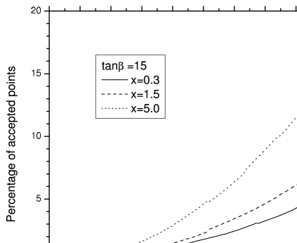
Figure 1: Analysis of the LFV decay $\mu\rightarrow e\,\gamma$ as a function of ${\widetilde{m}_{0}}$, using the MIAM and by randomly generating $10^{5}$ points for $(z^{l}_{LR})_{21}$ coefficient, assuming $\tan\beta=15$ for $x_{{\tilde{B}}}=0.3,\,1.5,\,5$. The different draw-lines show the fraction of such points that satisfies the current experimental bound $BR(\mu\rightarrow e\,\gamma)<1.2\times 10^{-11}$.

Now, our numerical analysis is based on a random generation of the parameters $(z^{l}_{LR})_{ij}$ ($10^{5}$ points are generated) and then studying their effects on the LFV transitions. Our results for $\mu\rightarrow e\,\gamma$ are shown in Fig. 1, assuming $\tan\beta=15$ for $x_{{\tilde{B}}}=0.3,1.5,5$.

Fig. 1 illustrates the severity of the SUSY flavor problem for low sfermion masses. One can see that even for ${\widetilde{m}_{0}}=1$ TeV almost $100\%$ of the randomly generated points are experimentally excluded, while one needs to have ${\widetilde{m}_{0}}\approx 10$ TeV in order to obtain that approximately $10\%$ of the generated points satisfy the current bound on $\mu\rightarrow e\,\gamma$. On other hand, larger gaugino masses help to ameliorate the problem, but not much. For instance, assuming $x_{{\tilde{B}}}=5$ and $\tan\beta=15$, implies that even for ${\widetilde{m}_{0}}=10$ TeV, the percentage of acceptable points only raises up to $18\%$.

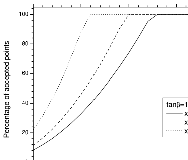
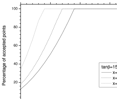
Figure 2: Analysis of the LFV decays $\tau\rightarrow\mu\,\gamma$ and $\tau\rightarrow e\,\gamma$ as a function of ${\widetilde{m}_{0}}$, using MIAM and by randomly generating $10^{5}$ points for (a)$(z^{l}_{LR})_{32}$ and (b) $(z^{l}_{LR})_{31}$ coefficients, assuming $\tan\beta=15$ and $x_{{\tilde{B}}}=0.3,\,1.5,\,5$. The different draw-lines show the fraction of such points that satisfies the current experimental bounds (a) $BR(\tau\rightarrow\mu\,\gamma)<1.1\times 10^{-6}$ and (b) $BR(\tau\rightarrow e\,\gamma)<2.7\times 10^{-6}$.

Current bounds on tau decays do not pose such severe problem, as is shown in Figs. 2. In this case most of the randomly generated points satisfy the bounds on $\tau\rightarrow\mu\,\gamma$ and $\tau\rightarrow e\,\gamma$. For instance, in the case of $\tau\rightarrow\mu\,\gamma$, with $x=0.3$ and $\tan\beta=15$ (see Fig. 2(a)); it is obtained that for $m_{\widetilde{l}}=200$ GeV approximately $10\%$ of the points are accepted by experimental data. However, this percentage increases with the slepton mass, and for $m_{\widetilde{l}}\geq 400$ GeV about $100\%$ of the points are accepted by experimental data. In Fig. 2(b), we notice that a similar behavior is obtained for $\tau\rightarrow e\,\gamma$. We can also notice in Fig. 2(a) (Fig. 2(b)) that for $x=0.5$ and $\tan\beta=15$ in the case $\tau\rightarrow\mu\,\gamma$ ($\tau\rightarrow e\,\gamma$) requires slepton masses, under $m_{\widetilde{l}}\geq 220$ GeV ($m_{\widetilde{l}}\geq 180$ GeV) in order to get $100\%$ of the points as acceptable by experimental data.

III The SUSY flavor problem beyond the mass-insertion approximation.

Now, we shall consider SUSY FCNC schemes where the general $6\times 6$ slepton-mass-matrix reduces down to a $4\times 4$ matrix involving only the $\tilde{\mu}-\tilde{\tau}$ sector, similarly to the quark sector discussed in Ref. oursqmix . In this case, $\tilde{\mu}-\tilde{\tau}$ flavor-mixings can be as large as $O(1)$. Although such large mixing could be related to the large $\nu_{\mu}-\nu_{\tau}$ mixing observed in atmospheric neutrinos superkam , we shall follow a bottom-up approach, where we simply take as an Ansatz the following form of the $A$-terms, taken also to be real and valid at the TeV-scale. Here, we consider two Ansatz kinds for $A$-terms, which are used for the diagonalization of fermion mass matrices.

III.1 Diagonalization of fermion mass matrices

1. Ansatz A

The reduction of the slepton mass matrix proceeds, for instance, by considering at the weak scale the following $A$-term (Ansatz A):

$$A_{l}=\left\lgroup\begin{array}[]{ccc}0&0&0\\ 0&0&z\\ 0&y&1\end{array}\right\rgroup A_{0}\,,$$ (12)

where $y$ and $z$ can be of $O(1)$, representing a naturally large flavor-mixing in the $\tilde{\mu}-\tilde{\tau}$ sector. Actually, the zero entries could be of $O(\epsilon)$, with $\epsilon\ll 1$, and their effect could be treated using the MIAM. Moreover, if we identify the non-diagonal $A_{l}$ as the only source of the observable LFV phenomena, this would implies that the slepton-mass-matrices $M_{{\widetilde{L}},{\widetilde{E}}}^{2}$ in Eqs. (2)-(3) to be nearly diagonal. For simplicity, we define

$$M_{LL}^{2}\,\simeq\,M_{RR}^{2}\,\simeq\,{\widetilde{m}_{0}}^{2}\,{\bf I}_{3\times 3}\,,$$ (13)

with ${\widetilde{m}_{0}}$ being a common scale for scalar-masses.

Within this minimal scheme, we observe that the first slepton family $\tilde{e}_{L,R}$ decouples from the rest in (2) so that, in the slepton basis $(\tilde{\mu}_{L},\,\tilde{\mu}_{R},\,\tilde{\tau}_{L},\,\tilde{\tau}_{R})$, the $6\times 6$ mass-matrix is reduced to the following $4\times 4$ matrix,

$${\widetilde{\cal M}}_{\tilde{l}}^{2}=\left\lgroup\begin{array}[]{cccc}~{}{{\widetilde{m}}}_{0}^{2}{}&0&0&A_{z}\\[2.84526pt] 0&~{}{\widetilde{m}}_{0}^{2}{}&A_{y}{}&0\\[2.84526pt] 0&A_{y}{}&~{}{\widetilde{m}}_{0}^{2}{}&X_{\tau}\\[2.84526pt] A_{z}{}&0&X_{\tau}{}&~{}{\widetilde{m}}_{0}^{2}\end{array}\right\rgroup$$ (14)

where

$$\begin{array}[]{l}A_{y}=y{\widehat{A}}\,,~{}~{}~{}A_{z}=z{\widehat{A}}\,,~{}~{}~{}{\widehat{A}}=Av\,{\cos\beta}/\sqrt{2}\,,~{}~{}~{}X_{\tau}={\widehat{A}}-\mu\,m_{\tau}\,{\tan\beta}\,.\\ \end{array}$$ (15)

The reduced slepton mass matrix (14) allows an exact diagonalization. Therefore, when evaluating loop amplitudes one can use the exact slepton mass-diagonalization and compare the results with those obtained from the popular but crude MIAM.

We now have obtained the mass-eigenvalues of the eigenstates $(\tilde{\mu}_{1},\,\tilde{\mu}_{2},\,\tilde{\tau}_{1},\,\tilde{\tau}_{2})$ for any $(y,\,z)$, given as:

$$\begin{array}[]{ll}M_{\tilde{\mu}_{1,2}}^{2}&={\widetilde{m}_{0}}^{2}\mp\frac{1}{2}|\sqrt{\omega_{+}}-\sqrt{\omega_{-}}|\,,\\[5.69054pt] M_{\tilde{\tau}_{1,2}}^{2}&={\widetilde{m}_{0}}^{2}\mp\frac{1}{2}|\sqrt{\omega_{+}}+\sqrt{\omega_{-}}|\,,\end{array}$$ (16)

where $~{}\omega_{\pm}=X_{\tau}^{2}+(A_{y}\pm A_{z})^{2}\,$. From (16), we can deduce the mass-spectrum of the $\tilde{\mu}-\tilde{\tau}$ sector as $M_{\tilde{\tau}_{1}}<M_{\tilde{\mu}_{1}}<M_{\tilde{\mu}_{2}}<M_{\tilde{\tau}_{2}}$.

The $4\times 4$ rotation matrix of the diagonalization is given by,

$$\begin{array}[]{l}\left\lgroup\begin{array}[]{l}\tilde{\mu}_{L}\\ \tilde{\mu}_{R}\\ \tilde{\tau}_{L}\\ \tilde{\tau}_{R}\end{array}\right\rgroup\!\!=\!\!\left\lgroup\begin{array}[]{rrrr}c_{1}c_{3}&c_{1}s_{3}&s_{1}s_{4}&s_{1}c_{4}\\ -c_{2}s_{3}&c_{2}c_{3}&s_{2}c_{4}&-s_{2}s_{4}\\ -s_{1}c_{3}&-s_{1}s_{3}&c_{1}s_{4}&c_{1}c_{4}\\ s_{2}s_{3}&-s_{2}c_{3}&c_{2}c_{4}&-c_{2}s_{4}\end{array}\right\rgroup\!\!\left\lgroup\begin{array}[]{l}\tilde{\mu}_{1}\\ \tilde{\mu}_{2}\\ \tilde{\tau}_{1}\\ \tilde{\tau}_{2}\end{array}\right\rgroup,\end{array}$$ (17)

with

$$~{}~{}~{}s_{1,2}=\displaystyle\frac{1}{{\sqrt{2}}}\left[1-\frac{X_{\tau}^{2}\mp A_{y}^{2}\pm A_{z}^{2}}{\sqrt{~{}\omega_{+}\omega_{-}}}\right]^{1/2}\!,~{}~{}~{}s_{4}=\frac{1}{{\sqrt{2}}}\,,$$ (18)

and $s_{3}=0\,(1/{\sqrt{2}})$ if $yz=0$($yz\neq 0$).

In Fig.3, we plot the slepton spectra as functions of $z$ for ${\widetilde{m}_{0}}=100,500$ GeV and ${\widetilde{m}_{0}}=1,10$ TeV, taking $\tan\beta=15$. We can observe that both $\tilde{\tau}_{1}$ and $\tilde{\tau}_{2}$ differ significantly from the common scalar mass ${\widetilde{m}_{0}}$; stau $\tilde{\tau}_{1}$ can be as light as about $100-300$ GeV, which have an important effect in the loop calculations. Furthermore, even for $z\simeq 0.5$ the smuon masses can differ from ${\widetilde{m}_{0}}$ for 30-50 GeV. With these mass values the slepton phenomenology would have to be reconsidered, since one is not allowed to sum over all the selectrons and smuons, for instance, when evaluating slepton cross-sections, as it is usually assumed in the constrained MSSM. We can also observe in Fig. 3 that $m_{\tilde{\mu}_{1}}-m_{\tilde{\tau}_{1}}$ and $m_{\tilde{\mu}_{2}}-m_{\tilde{\tau}_{2}}$ almost behave constant as one varies the parameter $z$ in the range $0\leq z\leq 1$. However, the differences $m_{\tilde{\mu}_{2}}-m_{\tilde{\mu}_{1}}$ and $m_{\tilde{\tau}_{2}}-m_{\tilde{\tau}_{1}}$ are sensitive to the non-minimal flavor structure. Besides, such splitting will affect the results for LFV transitions and the radiative fermion mass generation.

2. Ansatz B

Now, we will reduce the slepton mass matrix by considering another $A$-term at the weak scale (Ansatz B):

$$A_{l}=\left\lgroup\begin{array}[]{ccc}0&0&0\\ 0&w&y\\ 0&y&1\end{array}\right\rgroup A_{0}\,,$$ (19)

where $w$ and $y$ can be of $O(1)$, and as Ansatz A, the zero entries could be of $O(\epsilon)$, with $\epsilon\ll 1$. For this case, we take the same considerations of Ansatz A. Again, the first slepton family $\tilde{e}_{L,R}$ decouples from the rest in (2) and we obtain

$${\widetilde{\cal M}}_{\tilde{l}}^{2}=\left\lgroup\begin{array}[]{cccc}~{}{{\widetilde{m}}}_{0}^{2}{}&A_{w}{}&0&A_{y}\\[2.84526pt] A_{w}{}&~{}{\widetilde{m}}_{0}^{2}{}&A_{y}{}&0\\[2.84526pt] 0&A_{y}{}&~{}{\widetilde{m}}_{0}^{2}{}&X_{\tau}\\[2.84526pt] A_{y}{}&0&X_{\tau}{}&~{}{\widetilde{m}}_{0}^{2}\end{array}\right\rgroup$$ (20)

Here, $A_{w}=w{\widehat{A}}$, and $A_{y}$, ${\widehat{A}}$ and $X_{\tau}$ are the same of Eq (15).

For this case, mass-eigenvalues of the eigenstates $(\tilde{\mu}_{1},\,\tilde{\mu}_{2},\,\tilde{\tau}_{1},\,\tilde{\tau}_{2})$ for any $(w,\,y)$ have the following expressions:

$$\begin{array}[]{ll}M_{\tilde{\mu}_{1,2}}^{2}&=\frac{1}{2}(2{\widetilde{m}_{0}}^{2}\pm A_{w}\pm X_{\tau}\mp R),\\ M_{\tilde{\tau}_{1,2}}^{2}&=\frac{1}{2}(2{\widetilde{m}_{0}}^{2}\mp A_{w}\mp X_{\tau}\mp R),\end{array}$$

where $R=\sqrt{4A_{y}^{2}+\left(A_{w}-X_{\tau}\right)^{2}}$. From (III.1) and considering $\mu<0$, the mass-spectrum of the $\tilde{\mu}-\tilde{\tau}$ sector as $M_{\tilde{\tau}_{1}}<M_{\tilde{\mu}_{1}}<M_{\tilde{\mu}_{2}}<M_{\tilde{\tau}_{2}}$.

With this ansatz, the slepton spectra as functions of $y$ for ${\widetilde{m}_{0}}=100,500$ GeV, ${\widetilde{m}_{0}}=1,10$ TeV with $\tan\beta=15$, by considering $w=0.0,\,0.5,\,1.0$ have a similar behavior as in the case of Ansatz A.

By defining

$$\sin\phi=\frac{2A_{y}}{\sqrt{4A_{y}^{2}+(A_{w}-X_{\tau})^{2}}}\,,\mbox{\hskip 28.45274pt}\ \cos\phi=\frac{2A_{w}-X_{\tau}}{\sqrt{4A_{y}^{2}+(A_{w}-X_{\tau})^{2}}}\,,$$ (21)

the $4\times 4$ rotation matrix of the diagonalization is given by,

$$\begin{array}[]{l}\left\lgroup\begin{array}[]{l}\tilde{\mu}_{L}\\ \tilde{\mu}_{R}\\ \tilde{\tau}_{L}\\ \tilde{\tau}_{R}\end{array}\right\rgroup\!\!=\frac{1}{\sqrt{2}}\!\!\left\lgroup\begin{array}[]{rrrr}-s_{\xi}&s_{\xi}&-c_{\xi}&c_{\xi}\\ -s_{\xi}&-s_{\xi}&c_{\xi}&c_{\xi}\\ c_{\xi}&-c_{\xi}&-s_{\xi}&s_{\xi}\\ c_{\xi}&c_{\xi}&s_{\xi}&s_{\xi}\end{array}\right\rgroup\!\!\left\lgroup\begin{array}[]{l}\tilde{\mu}_{1}\\ \tilde{\mu}_{2}\\ \tilde{\tau}_{1}\\ \tilde{\tau}_{2}\end{array}\right\rgroup,\end{array}$$ (22)

where $s_{\xi}\equiv\sin(\phi/2)$ and $c_{\xi}\equiv\cos(\phi/2)$.

III.2 Gaugino-sfermion interactions

The interaction between gauginos and lepton-slepton pairs can be written as follows:

$${\cal{L}}_{int}=\overline{\chi}^{0}_{m}[\eta^{mL}_{\alpha k}P_{L}+\eta^{mR}_{\alpha k}P_{R}]\tilde{l}_{\alpha}l_{k}+h.c.,$$ (23)

where $\chi^{0}_{m}$ ($m=1,...,4$) denotes the neutralinos, while $\tilde{l}_{\alpha}$ correspond to the mass-eigenstate sleptons. The factors $\eta^{mN}_{\alpha k}$ are obtained after substituting the rotation matrices for both neutralinos and sleptons in the interaction lagrangian.

To carry out the forthcoming analysis of LFV transitions, we choose to work with the simplified case $y=z$, which gives: $c_{1}=c_{2}=c_{\tilde{l}}$, $s_{1}=s_{2}=s_{\tilde{l}}$ and $c_{3}=s_{3}=c_{4}=s_{4}=\frac{1}{\sqrt{2}}$. The expressions for $\eta^{mL,R}_{\alpha k}$ simplify further when the neutralino is taken as the bino, which we will assume in the calculation of Higgs LFV decays; the resulting coefficients ($\eta^{L,R}_{\alpha k}$) are shown in Table I.

$({\tilde{l}}_{\alpha},l_{k})$	$(\tilde{\mu}_{1},\mu)$	$(\tilde{\mu}_{1},\tau)$	$(\tilde{\mu}_{2},\mu)$	$(\tilde{\mu}_{2},\tau)$	$(\tilde{\tau}_{1},\mu)$	$(\tilde{\tau}_{1},\tau)$	$(\tilde{\tau}_{2},\mu)$	$(\tilde{\tau}_{2},\tau)$
$\eta^{L}_{\alpha k}$	$-c_{\tilde{l}}\frac{g_{1}}{2}$	$s_{\tilde{l}}\frac{g_{1}}{2}$	$-c_{\tilde{l}}\frac{g_{1}}{2}$	$s_{\tilde{l}}\frac{g_{1}}{2}$	$-s_{\tilde{l}}\frac{g_{1}}{2}$	$-c_{\tilde{l}}\frac{g_{1}}{2}$	$-s_{\tilde{l}}\frac{g_{1}}{2}$	$-c_{\tilde{l}}\frac{g_{1}}{2}$
$\eta^{R}_{\alpha k}$	$-c_{\tilde{l}}g_{1}$	$s_{\tilde{l}}g_{1}$	$-c_{\tilde{l}}g_{1}$	$-s_{\tilde{l}}g_{1}$	$s_{\tilde{l}}g_{1}$	$c_{\tilde{l}}g_{1}$	$-s_{\tilde{l}}g_{1}$	$-c_{\tilde{l}}g_{1}$

Table 1: Slepton-lepton-neutralino couplings ($\eta^{mN}_{\alpha k}$) for the case when $y=z$ and $\chi^{0}_{1}=\tilde{B}$.

III.3 Bounds on the LFV parameters from $\tau\rightarrow\mu+\gamma$

Here, we are interested in determining which fraction of points in parameter space satisfy current bounds on LFV tau decays, when the exact slepton mass-diagonalization is applied; again we generate $10^{5}$ random values of $O(1)$ for the parameter $z$ appearing in the soft-terms, and fix the values of $\widetilde{m}_{0}$, $\widetilde{M}$ and $\tan\beta$. Using interaction lagrangian (21) the one can write the general expressions for the SUSY contributions to the decays $\tau\rightarrow\mu+\gamma$ given in Ref. hisanoetal . The expression for $\Gamma(\tau\rightarrow\mu+\gamma)$, including the $\tilde{\mu}$ and $\tilde{\tau}$ contributions, is written as follows:

$$\Gamma(\tau\rightarrow\mu+\gamma)=\frac{\alpha m^{5}_{\tau}}{4\pi}[\sum_{\alpha}|A_{L\alpha}|^{2}+|A_{R\alpha}|^{2}],$$ (24)

where

$$A_{R\alpha}=\frac{1}{32\pi^{2}m^{2}_{{\tilde{l}}_{\alpha}}}[\eta^{R}_{{\tilde{l}}_{\alpha}\tau}\eta^{R}_{{\tilde{l}}_{\alpha}\mu}f_{1}(x_{\alpha})+\eta^{R}_{{slp}_{\alpha}\tau}\eta^{L}_{{\tilde{l}}_{\alpha}\mu}\frac{m_{\tilde{B}}}{m_{\tau}}f_{2}(x_{\alpha})],$$ (25)

with $x_{\alpha}=m^{2}_{\tilde{B}}/m^{2}_{{\tilde{l}}_{\alpha}}$, and the functions $f_{1,2}(x_{\alpha})$ are given in Ref. hisanoetal . $A_{L\alpha}$ is obtained by making the substitutions $L,R\rightarrow R,L$ in Eq.(23). The expressions for the $\Gamma(\mu\rightarrow e+\gamma)$ and $\Gamma(\tau\rightarrow e+\gamma)$ decays are still given by the MIAM.

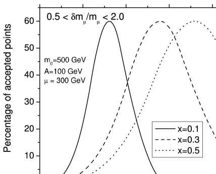
Figure 7: Radiative generation of the $m_{\mu}$ as a function of $\tan\beta$, using the FDM A and by generating $10^{5}$ random values for $y$ and $z$ with $x_{\tilde{\gamma}}=0.1,\,0.3,\,0.5$. The different draw-lines show the fraction of points that produce a correction that falls within the range $0.5<\delta m_{\mu}/m_{\mu}<2.0$.

The decay width depends on the SUSY parameters, and again we shall randomly generate the points and use the current bound $BR(\tau\rightarrow\mu+\gamma)<1.1\times 10^{-6}$ to determine which percentage is excluded/accepted. In Fig. 3, we can see that starting with values of the scalar mass parameter ${\widetilde{m}_{0}}\geq 460$ GeV, about $100\%$ of the generated points are acceptable for $x\geq 0.3$, see Fig. 7 (compare with the result ${\widetilde{m}_{0}}\geq 360$ GeV, obtained using MIAM).

IV Radiative Fermion masses in the MSSM

Understanding the origin of fermion masses and mixing angles is one of the main problems in Particle Physics. Because of the observed hierarchy, it is plausible to suspect that some of the entries in the full (non-diagonal) fermion mass matrices could be originate as a radiative effect. The MSSM loops involving sfermions and gauginos some of those entries could generate . However, most attempts presented so far Ferrandis:2004ng ; Ferrandis:2004ri ; Diaz-Cruz:2005qz ; Diaz-Cruz:2000mn could be seen as being highly dependent on the details of the SUSY breaking particular aspects. In this section we would like to scan the parameter space in order to determine which is the natural size of such corrections, namely to study which of the fermion masses could be generated in a natural manner. We shall concentrate on the charged lepton case, and will use both the MIAM as well as the FDM of a particular Ansatz for the soft-breaking trilinear terms.

IV.1 Mass-insertion approximation method (MIAM)

A Left-Right diagonal mass-insertion $(\delta_{ii})_{LR}=(\delta_{ii})_{RL}$ generates a one-loop mass term for leptons given by gabbiani

$$\delta m_{i}=-\frac{\alpha}{2\pi}\,m_{\tilde{\gamma}}\,Re(\delta_{ii})_{LR}\,I(x_{\tilde{\gamma}}),$$ (26)

where the function $I(x)$ is given by

$$I(x)=\frac{-1+x-x\ln(x)}{(1-x)^{2}}.$$ (27)

In our approximation

$$Re(\delta_{ii})_{LR}=\frac{\cos\beta}{\sqrt{2}}\frac{v}{{\widetilde{m}_{0}}},\,(z^{l}_{LR})_{ii}$$ (28)

hence

$$\delta m_{i}=-\frac{\alpha}{2\pi}\,I(x_{\tilde{\gamma}})\frac{\cos\beta}{\sqrt{2}}\,\sqrt{x_{\tilde{\gamma}}}\,v\,(z^{l}_{LR})_{ii}.$$ (29)

Again, $x_{\tilde{\gamma}}\equiv(m_{\tilde{\gamma}}/{\widetilde{m}_{0}})^{2}$ . Again, we shall generate $10^{5}$ random values of $O(1)$ for the parameter $(z^{l}_{LR})_{ii}$. In addition such points must satisfy the LFV current bounds. One can estimate the natural value of the fermion mass generated from SUSY loops, by taking $x_{\tilde{\gamma}}=0.3$, $\tan\beta=15-50$ and $(z^{l}_{LR})_{ii}\approx 1$, which gives $\delta m_{i}\approx 10-3$ MeV. Thus, in order to generate the $e$-$\mu$ hierarchy, one will need to include it in the $A$-terms, namely:

$$\frac{\delta m_{e}}{\delta m_{\mu}}=\frac{m_{e}}{m_{\mu}}\cong\frac{1}{200},$$

then

$$\frac{(z^{l}_{LR})_{11}}{(z^{l}_{LR})_{22}}\cong\frac{1}{200}.$$

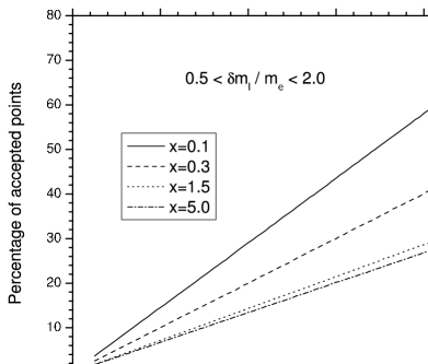
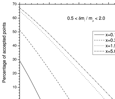
Figure 5: Radiative generation of the $m_{e}$ and $m_{\mu}$ as a function of $\tan\beta$, using MIAM and by generating $10^{5}$ random values for (a) $(z^{l}_{LR})_{11}$ and (b) $(z^{l}_{LR})_{22}$, with $x_{\tilde{\gamma}}=0.1,\,0.3,\,1.5,\,5$. The different draw-lines show the fraction of points that produce a correction that falls within the range $0.5<\delta m_{l}/m_{e},<\delta m_{l}/m_{\mu}<2.0$.

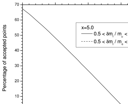
Figure 6: Radiative generation of the $m_{\mu}$ and $m_{e}$ as a function of $\tan\beta$, using MIAM and by generating $10^{5}$ random values for $(z^{l}_{LR})_{22}=(z^{l}_{LR})_{11}$ with $x_{\tilde{\gamma}}=5$. The solid draw-line shows the fraction of points that produce a correction that falls within the range $0.5<\delta m_{l}/m_{\mu}<2.0$, while the dashed one shows the fraction of points that produce a correction that falls within the range $0.5<\delta m_{l}/m_{e}<2.0$.

Such hierarchy can only arise as a result of some flavor symmetry. Thus, one can see that radiative mechanism requires an additional input in order to reproduce the observed fermion masses. The percentage of points that produce a correction that falls within the range $0.5<\delta m_{e}/m_{e}<2.0$ as a function of $\tan\beta$, for $x_{\tilde{\gamma}}=0.1,0.3,1.5,5.0$, is shown in Fig. 5(a); the percentage of points that produce a correction that falls within the range $0.5<\delta m_{\mu}/m_{\mu}<2.0$ as a function of $\tan\beta$, for $x_{\tilde{\gamma}}=0.1$ is plotted in Fig 5(b), $x_{\tilde{\gamma}}=0.3$, $x_{\tilde{\gamma}}=1.5$ and $x_{\tilde{\gamma}}=5$. We numerically observed that it is not possible to generate the tau mass (it can be shown that at least one fermion should have a mass in order to radiatively generate the rest). Numerically, we have found that it is possible to find a set of parameters $x_{\tilde{\gamma}}$ and $\tan\beta$ for which the fraction of points that produce a correction that falls simultaneously within the range $0.5<\delta m_{e}/m_{e}<2.0$ and $0.5<\delta m_{\mu}/m_{\mu}<2.0$ is small, but different from zero, as it is shown in Fig. 6.

It can be noticed that without further theoretical input the values of $(z^{l}_{LR})_{ii}$ do not make distinction between the families. For the electron mass, one needs higher values of $\tan\beta$ in order to get a significant fraction of points (bigger than 10%) where the electron mass is generated. For lower values of $\tan\beta$, what happen that the mass generated exceeds the range ($0.5<\delta m_{e}/m_{e}<2.0$).

IV.2 Exact diagonalization of a particular Ansatz and the one loop correction

1. Ansatz A

When one uses the exact diagonalization, one can identify the dominant finite one loop contribution to the lepton mass correction $\delta m_{l}$. It is given by

$$(\delta m_{l})_{ab}=\frac{\alpha}{2\pi}m_{\tilde{B}}\sum_{c}Z_{ca}^{l}Z_{c(b+3)}^{l*}B_{0}(m_{\tilde{B}},m_{\tilde{l}_{c}})$$ (30)

where $l_{c}$ ($c=4,5,6$)are the lepton left mass eigenstates ($c=1,2,3$) and the lepton right mass eigenstates . The selectrons can be decoupled with no flavor mixing with the $\tilde{\mu}-\tilde{\tau}$ sector, then the sfermion matrix is diagonalized by an unitary matrix, $Z^{l}$, which is given on the basis $(\tilde{e}_{L},\tilde{\mu}_{L},\tilde{\tau}_{L},\tilde{e}_{R},\tilde{\mu}_{R},\tilde{\tau}_{R})$ as follows:

$$\begin{array}[]{l}\left\lgroup\begin{array}[]{l}\tilde{e}_{L}\\ \tilde{\mu}_{L}\\ \tilde{\tau}_{L}\\ \tilde{e}_{R}\\ \tilde{\mu}_{R}\\ \tilde{\tau}_{R}\end{array}\right\rgroup\!\!=\!\!\left\lgroup\begin{array}[]{rrrrrr}1&0&0&0&0&0\\ 0&c_{1}c_{3}&s_{1}s_{4}&0&c_{1}s_{3}&s_{1}c_{4}\\ 0&-s_{1}c_{3}&c_{1}s_{4}&0&-s_{1}s_{3}&c_{1}c_{4}\\ 0&0&0&1&0&0\\ 0&-c_{2}s_{3}&s_{2}c_{4}&0&c_{2}c_{3}&-s_{2}s_{4}\\ 0&s_{2}s_{3}&c_{2}c_{4}&0&-s_{2}c_{3}&-c_{2}s_{4}\end{array}\right\rgroup\!\!\left\lgroup\begin{array}[]{l}\tilde{e}_{1}\\ \tilde{\mu}_{1}\\ \tilde{\tau}_{1}\\ \tilde{e}_{2}\\ \tilde{\mu}_{2}\\ \tilde{\tau}_{2}\end{array}\right\rgroup,\end{array}$$ (31)

with $s_{1,2,3,4}$ defined in Eq. (18).

From the rotation matrix (31), we see that matrix elements $(\delta m_{l})_{a1}=(\delta m_{l})_{1b}=0$, therefore only the muon mass can be entirely generated from loop corrections. The rest of the matrix element are given as follows:

$$\begin{array}[]{rcl}(\delta m_{l})_{22}&=&\frac{\alpha}{4\pi}m_{\tilde{B}}\left\{[c_{1}^{2}B_{0}(m_{\tilde{B}},m_{{\tilde{\mu}}_{1}})-c_{2}^{2}B_{0}(m_{\tilde{B}},m_{{\tilde{\mu}}_{2}})]+[s_{1}^{2}B_{0}(m_{\tilde{B}},m_{{\tilde{\tau}}_{1}})-s_{2}^{2}B_{0}(m_{\tilde{B}},m_{{\tilde{\tau}}_{2}})]\right\},\\ (\delta m_{l})_{23}&=&\frac{\alpha}{4\pi}m_{\tilde{B}}\left\{c_{1}s_{1}[B_{0}(m_{\tilde{B}},m_{{\tilde{\mu}}_{1}})-B_{0}(m_{\tilde{B}},m_{{\tilde{\tau}}_{1}})]+c_{2}s_{2}[B_{0}(m_{\tilde{B}},m_{{\tilde{\mu}}_{2}})-B_{0}(m_{\tilde{B}},m_{{\tilde{\tau}}_{2}})]\right\},\\ (\delta m_{l})_{32}&=&(\delta m_{l})_{23},\\ (\delta m_{l})_{33}&=&\frac{\alpha}{4\pi}m_{\tilde{B}}\left\{[s_{1}^{2}B_{0}(m_{\tilde{B}},m_{{\tilde{\mu}}_{1}})-s_{2}^{2}B_{0}(m_{\tilde{B}},m_{{\tilde{\mu}}_{2}})]+[c_{1}^{2}B_{0}(m_{\tilde{B}},m_{{\tilde{\tau}}_{1}})-c_{2}^{2}B_{0}(m_{\tilde{B}},m_{{\tilde{\tau}}_{2}})]\right\},\end{array}$$ (32)

where

$$B_{0}(m,m_{i})-B_{0}(m,m_{j})=\ln\left(\frac{m_{j}^{2}}{m_{i}^{2}}\right)+\frac{m^{2}}{m_{i}^{2}-m^{2}}\ln\left(\frac{m_{i}^{2}}{m^{2}}\right)-\frac{m^{2}}{m_{j}^{2}-m^{2}}\ln\left(\frac{m_{j}^{2}}{m^{2}}\right)$$

which follows from

$$B_{0}(m_{1},m_{2})=1+\ln\left(\frac{Q^{2}}{m_{2}^{2}}\right)+\frac{m_{1}^{2}}{m_{2}^{2}-m_{1}^{2}}\ln\left(\frac{m_{2}^{2}}{m_{1}^{2}}\right).$$

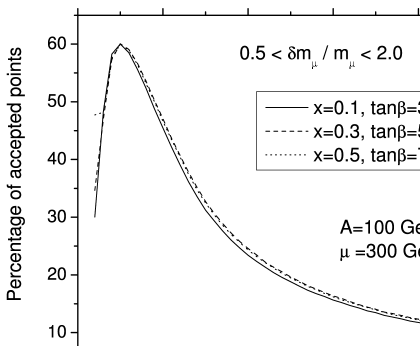
Figure 8: Radiative generation of the muon mass as a function of ${\widetilde{m}_{0}}$, using the FDM A and by generating $10^{5}$ random values for $y$ and $z$, with: a) $x_{\tilde{\gamma}}=0.1$ and $\tan\beta=32$, b) $x_{\tilde{\gamma}}=0.3$ and $\tan\beta=56$, c) $x_{\tilde{\gamma}}=0.5$ and $\tan\beta=72$. The different draw-lines show the fraction of points that produce a correction that falls within the range $0.5<\delta m_{\mu}/m_{\mu}<2.0$.

After generating $10^{5}$ random values of $O(1)$ for the parameters $y$ and $z$, we show our results in Figs. 7 and 8. In Fig. 7 is shown the percentage of points that produce a correction that falls within the range $0.5<\delta m_{\mu}/m_{\mu}<2.0$ as a function of $\tan\beta$, for $x_{\tilde{\gamma}}=0.1$, $x_{\tilde{\gamma}}=0.3$ and $x_{\tilde{\gamma}}=0.5$. We notice that a high $\tan\beta$ range is required to get a correct generation. In Fig. 8 is plotted the percentage of points that produce a correction that falls within the range $0.5<\delta m_{\mu}/m_{\mu}<2.0$ as a function of ${\widetilde{m}_{0}}$, for $x_{\tilde{\gamma}}=0.1$ and $\tan\beta=32$, $x_{\tilde{\gamma}}=0.3$ and $\tan\beta=56$, $x_{\tilde{\gamma}}=0.5$ and $\tan\beta=72$. We find that a slepton mass parameter ${\widetilde{m}_{0}}\lower 3.01385pt\hbox{$\;\stackrel{{\scriptstyle\textstyle<}}{{\sim}}\;$}1$ TeV is required in order to generate the muon mass for about 40-60% of generated points.

Ansatz B

As we have already mentioned in Subsection IV.B, when we use the exact diagonalization, we can identify the dominant finite one loop contribution to the lepton mass correction $\delta m_{l}$, which is given by Eq.(30). Using the Ansatz B (Eq.(19)), the sfermion matrix is diagonalized by an unitary matrix, $Z^{l}_{B}$, which is given, in the basis $(\tilde{e}_{L},\tilde{\mu}_{L},\tilde{\tau}_{L},\tilde{e}_{R},\tilde{\mu}_{R},\tilde{\tau}_{R})$, as:

$$\begin{array}[]{l}\left\lgroup\begin{array}[]{l}\tilde{e}_{L}\\ \tilde{\mu}_{L}\\ \tilde{\tau}_{L}\\ \tilde{e}_{R}\\ \tilde{\mu}_{R}\\ \tilde{\tau}_{R}\end{array}\right\rgroup\!\!=\frac{1}{\sqrt{2}}\!\!\left\lgroup\begin{array}[]{rrrrrr}1&0&0&0&0&0\\ 0&-s_{\xi}&-c_{\xi}&0&s_{\xi}&c_{\xi}\\ 0&c_{\xi}&-s_{\xi}&0&-c_{\xi}&s_{\xi}\\ 0&0&0&1&0&0\\ 0&-s_{\xi}&c_{\xi}&0&-s_{\xi}&c_{\xi}\\ 0&c_{\xi}&s_{\xi}&0&c_{\xi}&s_{\xi}\\ \end{array}\right\rgroup\!\!\left\lgroup\begin{array}[]{l}\tilde{e}_{1}\\ \tilde{\mu}_{1}\\ \tilde{\tau}_{1}\\ \tilde{e}_{2}\\ \tilde{\mu}_{2}\\ \tilde{\tau}_{2}\end{array}\right\rgroup,\end{array}$$ (33)

with $s_{\xi}\equiv\sin(\phi/2)$ and $c_{\xi}\equiv\cos(\phi/2)$ (see Eq.(21)).

From the rotation matrix (33), we see that matrix elements $(\delta m_{l})_{a1}=(\delta m_{l})_{1b}=0$, therefore only the $\mu$ mass can be entirely generated from loop corrections. The rest of the matrix element are given as follows:

$$(\delta m_{l})_{22} = \frac{\alpha}{4\pi}m_{\tilde{B}}\left\{s^{2}_{\xi}[B_{0}(m_{\tilde{B}},m_{{\tilde{\mu}}_{2}})-B_{0}(m_{\tilde{B}},m_{{\tilde{\mu}}_{1}})]+c^{2}_{\xi}[B_{0}(m_{\tilde{B}},m_{{\tilde{\tau}}_{2}})-B_{0}(m_{\tilde{B}},m_{{\tilde{\tau}}_{1}})]\right\}$$

$$(\delta m_{l})_{23} = \frac{\alpha}{4\pi}m_{\tilde{B}}\left\{s_{\xi}c_{\xi}[B_{0}(m_{\tilde{B}},m_{{\tilde{\tau}}_{2}})-B_{0}(m_{\tilde{B}},m_{{\tilde{\mu}}_{2}})]+s_{\xi}c_{\xi}[B_{0}(m_{\tilde{B}},m_{{\tilde{\tau}}_{1}})+B_{0}(m_{\tilde{B}},m_{{\tilde{\mu}}_{1}})]\right\}$$

$$(\delta m_{l})_{32} = (\delta m_{l})_{23}$$ (34)

$$(\delta m_{l})_{33} = \frac{\alpha}{4\pi}m_{\tilde{B}}\left\{c_{\xi}^{2}[B_{0}(m_{\tilde{B}},m_{{\tilde{\mu}}_{2}})-B_{0}(m_{\tilde{B}},m_{{\tilde{\mu}}_{1}})]+s_{\xi}^{2}[B_{0}(m_{\tilde{B}},m_{{\tilde{\tau}}_{2}})-B_{0}(m_{\tilde{B}},m_{{\tilde{\tau}}_{1}})]\right\}\,,$$

where $B_{0}(m,m_{i})-B_{0}(m,m_{j})$ and $B_{0}(m_{1},m_{2})$ are given in the previous Subsection (IV.B).

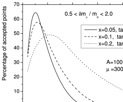
Figure 10: Radiative generation of the muon mass as a function of ${\widetilde{m}_{0}}$, using the FDM B and by generating $10^{5}$ random values for $w$ and $y$, with: a) $x_{\tilde{\gamma}}=0.05$, $\tan\beta=3.2$, b) $x_{\tilde{\gamma}}=0.1$, $\tan\beta=4.2$ and c) $x_{\tilde{\gamma}}=0.2$, $\tan\beta=4.7$. The different draw-lines show the fraction of points that produce a correction that falls within the range $0.5<\delta m_{\mu}/m_{\mu}<2.0$.

After generating $10^{5}$ random values of $O(1)$ for the parameters $w$ and $y$, we show our results in Figs. 9 and 10. In Fig. 9 is shown the percentage of points that produce a correction that falls within the range $0.5<\delta m_{\mu}/m_{\mu}<2.0$ as a function of $\tan\beta$, for $x_{\tilde{\gamma}}=0.05$, $x_{\tilde{\gamma}}=0.1$ and $x_{\tilde{\gamma}}=0.2$. We notice that a $0\lower 3.01385pt\hbox{$\;\stackrel{{\scriptstyle\textstyle<}}{{\sim}}\;$}\tan\beta\lower 3.01385pt\hbox{$\;\stackrel{{\scriptstyle\textstyle<}}{{\sim}}\;$}10$ range is required to get a correct generation. The percentage of points that produce a correction that falls within the range $0.5<\delta m_{\mu}/m_{\mu}<2.0$ as a function of ${\widetilde{m}_{0}}$, for $x_{\tilde{\gamma}}=0.05$ and $\tan\beta=3.2$, $x_{\tilde{\gamma}}=0.1$ and $\tan\beta=4.2$, $x_{\tilde{\gamma}}=0.2$ and $\tan\beta=4.7$, is plotted in Fig. 10. We found that a slepton mass parameter ${\widetilde{m}_{0}}\lower 3.01385pt\hbox{$\;\stackrel{{\scriptstyle\textstyle<}}{{\sim}}\;$}1$ TeV is required in order to generate the muon mass for about 40-65% of the generated points.

V Conclusions

We have discussed the SUSY flavor problem in the lepton sector using the mass-insertion approximation, evaluating the radiative LFV loop transitions ($l_{i}\rightarrow l_{j}\gamma$) with a random generation of the slepton $A$-terms. Our results illustrate the severity of the SUSY flavor problem for low sfermion masses. One can see that even for ${\widetilde{m}_{0}}=1$ TeV almost $100\%$ of the randomly generated points are excluded, while one needs to have ${\widetilde{m}_{0}}\approx 10$ TeV in order to get about $10\%$ of the generated points that satisfy the current bound on $\mu\rightarrow e\,\gamma$, having larger gaugino helps to ameliorate the problem, but not by much. On the other hand, we have shown that current bounds on tau decays pose no such a severe problem. In this case, most of the randomly generated points satisfy the experimental bounds on $\tau\rightarrow\mu\,\gamma$ and $\tau\rightarrow e\,\gamma$. Also, we presented two Ansaetze for soft breaking trilinear terms, the diagonalization of the resulting sfermion mass matrices, and repeat the previous calculation. We showed that for ${\widetilde{m}_{0}}\geq 460$ GeV, $100\%$ of the points are acceptable for $x_{\tilde{\gamma}}\geq 0.3$, with similar behavior in both cases (to be compared with ${\widetilde{m}_{0}}\geq 360$ GeV obtained using the mass-insertion approximation).

The radiative generation of fermion masses within the context of the MSSM with general trilinear soft-breaking terms was discussed in detail. We presented results for slepton spectra for ${\widetilde{m}_{0}}=100,500$ GeV and ${\widetilde{m}_{0}}=1,10$ TeV, with $\tan\beta=15$, showing that both $\tilde{\tau}_{1}$ and $\tilde{\tau}_{2}$ differ significantly from ${\widetilde{m}_{0}}$. Moreover, $\tilde{\tau}_{1}$ can be as light as $100-300$ GeV, which will have an important effect in the loop calculations. Furthermore, $m_{\tilde{\mu}_{i}}$ can differ from ${\widetilde{m}_{0}}$ for 30-50 GeV considering $z\simeq 0.5$; with these mass values the slepton phenomenology would have to be reconsidered. We also observed that $m_{\tilde{\mu}_{1}}-m_{\tilde{\tau}_{1}}$ and $m_{\tilde{\mu}_{2}}-m_{\tilde{\tau}_{2}}$ almost behave constant as one varies the parameter $z$ in the range $0\leq z\leq 1$. This splitting affects LFV transitions and radiative fermion mass generation results.

Also, we have analyzed the radiative generation of the $e$ and $\mu$ masses using the MIAM by generating $10^{5}$ random values of $O(1)$ for the parameters $(z^{l}_{LR})_{ii}$. It was shown that for some parameters a percentage of points may produce a correction that falls within the range $0.5<\delta m_{l}/m_{e}<2$, while another percentage of points can produce a correction that falls within the range $0.5<\delta m_{l}/m_{\mu}<2$. Then, it is possible to find a set of parameters $x$ and $\tan\beta$ for which the fraction of points that produce a correction that falls simultaneously within the range $0.5<\delta m_{e}/m_{e},\delta m_{\mu}/m_{\mu}<2.0$, which is small, but different from zero. Numerically concluding that it is not possible to generate the tau mass. Having noticed that without further theoretical input the values of $(z^{l}_{LR})_{ii}$ do not distinguish among the families. For the electron mass, one needs higher values of $\tan\beta$ in order to get a significant fraction of points (bigger than 10%) where the electron mass is generated. For lower values of $\tan\beta$, what happens is that the mass generated exceeds the range ($0.5<\delta m_{e}/m_{e}<2.0$).

We have pointed out that in order to generate the $e$-$\mu$ hierarchy, one needs to have $(z^{l}_{LR})_{11}/(z^{l}_{LR})_{22}\cong 1/200$. Such hierarchy can only arise as a result of some flavor symmetry. Thus, one can conclude that the radiative mechanism requires an additional input in order to reproduce the observed fermion masses.

On the other hand, we have analyzed the radiative generation of the muon mass using a FDM, by considering at the weak scale two different Ansaetze for $A$-term, by generating $10^{5}$ random values of $O(1)$ for the parameters $y$ and $z$ of the model. It is shown that for some parameters a percentage of points may produce a correction that falls within the range $0.5<\delta m_{\mu}/m_{\mu}<2$, watching a quite different behavior from the resulting fractions of acceptable points when we consider the different Ansaetze as well as with the two full diagonalization models and the mass-insertion approximation. Similarly to the mass-insertion approximation case, it is not numerically possible to radiatively generate the tau mass by using the two full diagonalization models considered.

Acknowledgments

We would like to thank C.P. Yuan and H.J. He for valuable discussions. This work was supported in part by CONACYT and SNI (México).

Figure 3: Mass spectrum for the smuon and stau sleptons as a function of $z$ for ${\tan\beta}=15$ and the SUSY scale (a) ${\widetilde{m}_{0}}=100$ GeV, (b) ${\widetilde{m}_{0}}=500$ GeV, (c) ${\widetilde{m}_{0}}=1$ TeV and (d) ${\widetilde{m}_{0}}=10$ TeV.

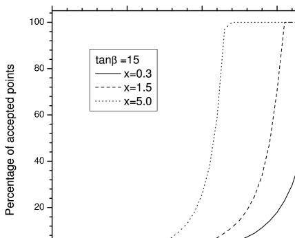
Figure 4: Analysis of the LFV decay $\tau\rightarrow\mu\,\gamma$ as a function of ${\widetilde{m}_{0}}$, using a FDM and by randomly generating $10^{5}$ points for $z$ coefficient, assuming $\tan\beta=15$ and $x_{{\tilde{B}}}=0.3,\,1.5,\,5$. The different draw-lines show the fraction of such points that satisfies the current experimental bound $BR(\tau\rightarrow\mu\,\gamma)<1.1\times 10^{-6}$.

Figure 9: Radiative generation of the muon mass as a function of $\tan\beta$, using the FDM B and by generating $10^{5}$ random values for $w$ and $y$, with $x_{\tilde{\gamma}}=0.05,\,0.1,\,0.2$. The different draw-lines show the fraction of points that produce a correction that falls within the range $0.5<\delta m_{\mu}/m_{\mu}<2.0$.

References

- (1) See, for instance, recent reviews in “Perspectives on Supersymmetry”, ed. G. L. Kane, World Scientific Publishing Co., 1998; H. E. Haber, Nucl. Phys. Proc. Suppl. 101, 217 (2001), [hep-ph/0103095].
- (2) D. J. H. Chung, L. L. Everett, G. L. Kane, S. F. King, J. D. Lykken and L. T. Wang, Phys. Rept. 407, 1 (2005), [hep-ph/0312378].
- (3) E.g., S. Khalil, J. Phys. G27, 1183 (2001), [hep-ph/0011330]; D. F. Carvalho, M. E. Gomez, S. Khalil, [hep-ph/0104292]; and references therein.
- (4) A. Masiero and H. Murayama, Phys. Rev. Lett. 83, 907 (1999), [hep-ph/9903363].
- (5) F. Gabbiani, E. Gabrielli, A. Masiero and L. Silvestrini, Nucl. Phys. B 477, 321 (1996).
- (6) N. Arkani-Hamed and H. Murayama, Phys. Rev. D 56, 6733 (1997), [hep-ph/9703259].
- (7) E.g., Y. Nir and N. Seiberg, Phys. Lett. B 309, 337 (1993), [hep-ph/9304307].
- (8) For review, M. Misiak, S. Pokorski, J. Rosiek, “Supersymmetry and FCNC Effects”, [hep-ph/9703442], in Heavy Flavor II, pp. 795, Eds. A. J. Buras and M. Lindner, Advanced Series on Directions in High Energey Physics, World Scientific Publishing Co., 1998, and references therein.
- (9) J. L. Diaz-Cruz, H. J. He and C. P. Yuan, “Soft SUSY breaking, stop-scharm mixing and Higgs signatures,” Phys. Lett. B 530, 179 (2002), [hep-ph/0103178].
- (10) Super-Kamiokande Collaboration (Y. Fukuda et al.), Phys. Rev. Lett. 81, 1562 (1998), [hep-ex/0009001].
- (11) P. Paradisi, JHEP 0510, 006 (2005), [hep-ph/0505046].
- (12) J. L. Diaz-Cruz, JHEP 0305, 036 (2003), [hep-ph/0207030].
- (13) J. L. Diaz-Cruz and J. J. Toscano, Phys. Rev. D 62, 116005 (2000), [hep-ph/9910233].
- (14) J. A. Casas and S. Dimopolous, Phys. Lett. B 387, 107 (1996), [hep-ph/9606237].
- (15) S. Eidelman et al., (Review of Particle Physics), Phys. Lett. B 592, 1 (2004).
- (16) J. Hisano, T. Moroi, K. Tobe and M. Yamaguchi, “Lepton-Flavor Violation via Right-Handed Neutrino Yukawa Couplings in Supersymmetric Standard Model,” Phys. Rev. D 53, 2442 (1996), [hep-ph/9510309].
- (17) J. Ferrandis, Phys. Rev. D 70, 055002 (2004), [hep-ph/0404068].
- (18) J. Ferrandis and N. Haba, Phys. Rev. D 70, 055003 (2004), [hep-ph/0404077].
- (19) J. L. Diaz-Cruz and J. Ferrandis, Phys. Rev. D 72, 035003 (2005), [hep-ph/0504094].
- (20) J. L. Diaz-Cruz, H. Murayama and A. Pierce, Phys. Rev. D 65, 075011 (2002), [hep-ph/0012275].