hep-ph/0512169

CLNS-05/1941

FERMILAB-PUB-05-536-T

The flavor of a little Higgs with T-parity

Jay Hubisz^a, Seung J. Lee^b, Gil Paz^b

^a Fermi National Accelerator Laboratory,
P.O. Box 500, Batavia, IL 60510

^b Institute for High Energy Phenomenology, Laboratory of Elementary Particle Physics,
Cornell University, Ithaca, NY 14853

hubisz@fnal.gov, sjl18@cornell.edu, gilpaz@lepp.cornell.edu

We analyze flavor constraints in the littlest Higgs model with T-parity. In particular, we focus on neutral meson mixing in the $K$, $B$, and $D$ systems due to one loop contributions from T-parity odd fermions and gauge bosons. We calculate the short distance contributions to mixing for a general choice of T-odd fermion Yukawa couplings. We find that for a generic choice of textures, a TeV scale GIM suppression is necessary to avoid large contributions. If order one mixing angles are allowed in the extended flavor structure, the mass spectrum is severely constrained, and must be degenerate at the $1$-$5$% level. However, there are still regions of parameter space where only a loose degeneracy is necessary to avoid constraints. We also consider the $B_{s}$ system, and identify a scenario in which the mixing can be significantly enhanced beyond the standard model prediction while still satisfying bounds on the other mixing observables. We present both analytical and numerical results as functions of the T-odd fermion mass eigenvalues.

1 Introduction

The mechanism of electroweak symmetry breaking (EWSB) will presumably be revealed in the coming years through a combination of LHC and ILC data. It is expected that embedded in the newly discovered physics will be an explanation of how this mechanism remains stable under quantum corrections. Until this time, it is vital that we study the different known field theoretical mechanisms of EWSB that stabilize the Higgs potential.

The little Higgs mechanism [2, 3] is a revival of composite Higgs models [4, 5] that attempted to solve these issues. In these models, the Higgs is a pseudo-Goldstone boson of approximate global symmetries that are added on to the standard model (SM). In the little Higgs mechanism, the electroweak scale is stabilized against quadratically divergent corrections by the manner in which perturbative couplings break the global symmetries. In the simplest models, the Higgs mass receives no quadratically divergent quantum corrections until two loop order, although models with a larger symmetry structure can postpone these corrections to higher loop order [2].

The most compact implementation of the little Higgs mechanism is known as the littlest Higgs model [6]. In this model, the SM is enlarged to incorporate an approximate $SU(5)$ global symmetry. This symmetry is broken down to $SO(5)$ spontaneously, though the mechanism of this breaking is left unspecified. The Higgs is an approximate Goldstone boson of this breaking.

While the earliest littlest Higgs models have issues with low energy constraints [7], recent studies have shown that this structure is still possible if one adds a discrete $Z_{2}$ symmetry to the model [8]. Known as T-parity, this symmetry forbids the couplings which led to stringent electroweak precision and compositeness bounds in the original littlest Higgs model.

A consistent and phenomenologically viable littlest Higgs model with T-parity requires the introduction of “mirror fermions” [9]. For each new SM doublet, there must be another doublet which has the opposite T-parity eigenvalue. These mirror fermions are required to cut off otherwise large four-fermion operators constrained primarily by LEP, and Drell-Yan processes [10], but they also open up a new flavor structure in the model. From studies of supersymmetry and other models of new physics, it is known that new flavor structure at the TeV scale is quite stringently constrained [11]. This is primarily due to the presence, in the SM, of a GIM mechanism [12]. The lightness of the SM fermions, coupled with the near diagonal texture of the CKM matrix, strongly suppress flavor and CP violating amplitudes, pushing them well below their naive dimension analysis (NDA) estimated values. In the absence of a TeV scale GIM mechanism, new contributions to neutral meson mixing and rare decays are often many orders of magnitude larger than the SM contributions [13, 14].

Neutral meson mixing, CP violation, and rare decays have been tested experimentally through a variety of different observables, and are not substantially different than expectations derived from SM calculations. Therefore we expect there to be very little freedom in the new flavor sector. In this paper, we study the flavor constraints on the extended T-odd fermion sector of the littlest Higgs model with T-parity. Specifically, we consider constraints from neutral meson particle anti-particle mixing, leaving rare decays for future study.

In Section 2, we outline the conventions used to derive the Feynman rules relevant to flavor physics. In Section 3, we discuss how we approach the process of diagonalizing the action to the mass eigenbasis, and identify the new parameters which describe the new sources of flavor mixing and CP violation. In Section 4, we outline the calculations for neutral meson mixing in the SM. In Section 5, the contributions to neutral meson mixing involving the T-odd fields is presented. Section 6 contains a numerical analysis of the bounds on the parameters describing the T-odd fermion sector, and an analysis of $B_{s}$ mixing. We conclude in Section 7. In the Appendix, we give the relevant Feynman rules, as well as the formulas which arise from calculating the one loop contributions to flavor changing operators.

2 The Model

The littlest Higgs model [6] is the most compact way of extending the SM to include a collective symmetry breaking structure that protects the Higgs mass. In the littlest Higgs model, the theory is approximately invariant under $SU(5)$ global symmetry transformations. A scalar VEV of an $SU(5)$ symmetric tensor $\Sigma$ spontaneously breaks this $SU(5)$ down to $SO(5)$ at a scale $f$. This scale is presumed to be $\mathcal{O}(1\ \mathrm{TeV})$. The Higgs boson is one of the Goldstone bosons associated with this breaking. An $\left[SU(2)\times U(1)\right]^{2}$ subgroup embedded in the global $SU(5)$ is gauged, and after $\Sigma$ gets a VEV, this gauge symmetry is reduced to the SM $SU(2)_{L}\times U(1)_{Y}$. Perturbative couplings in the model break the $SU(5)$ global symmetry explicitly, and quantum corrections involving these interactions generate masses and non-derivative couplings for the Goldstone fluctuations, rendering them pseudo-Goldstone bosons.

The Higgs mass is protected from quadratic divergences at the one-loop level due to the way in which perturbative couplings are introduced. Any single coupling preserves at least one of two overlapping $SU(3)$ subgroups of the full $SU(5)$ global symmetry. Under these $SU(3)$ subgroups, the Higgs is still an exact Goldstone boson. The VEV which breaks the $SU(5)$ softly breaks these $SU(3)$ symmetries, and thus generates logarithmically divergent contributions to the Higgs mass at one loop. Amplitudes involving perturbative couplings only generate a quadratically divergent contribution at two loop order. The value for the Higgs mass obtained by NDA arguments is then suppressed relative to the breaking scale $f$ by a loop factor.

The effective action is parametrized by a non-linear sigma model. Only the Goldstone bosons of the $SU(5)$ breaking are included in the low energy effective theory, and the way in which the theory is linearized, or UV completed, is left ambiguous. In terms of these Goldstone fields, the symmetric tensor $\Sigma$ can be expressed as:

$$\Sigma=e^{2i\Pi/f}\Sigma_{0}.$$ (2.1)

The “pion” matrix $\Pi$ contains the Goldstone degrees of freedom, and $\Sigma_{0}$ is the VEV of $\Sigma$:

$$\Sigma_{0}=\left(\begin{array}[]{ccccc}0&0&0&1&0\\ 0&0&0&0&1\\ 0&0&1&0&0\\ 1&0&0&0&0\\ 0&1&0&0&0\end{array}\right).$$

To implement the collective symmetry breaking structure, the gauge generators are embedded in the $SU(5)$ global symmetry such that any given generator commutes with an $SU(3)$ subgroup of the $SU(5)$ global symmetry:

$$Q_{1}^{a}=\left(\begin{array}[]{ccc}\sigma^{a}/2&0&0\\ 0&0&0\\ 0&0&0\end{array}\right),\ \ \ Y_{1}={\rm diag}(3,3,-2,-2,-2)/10$$ (2.5)

$$Q_{2}^{a}=\left(\begin{array}[]{ccc}0&0&0\\ 0&0&0\\ 0&0&-\sigma^{a*}/2\end{array}\right), Y_{2}={\rm diag}(2,2,2,-3,-3)/10~{}.$$ (2.9)

The $Q_{1}$ and $Y_{1}$ generators commute with the $SU(3)_{2}$ subgroup of $SU(5)$ whose generators occupy the lower right hand corner. The $Q_{2}$ and $Y_{2}$ generators similarly commute with the $SU(3)_{1}$ subgroup in the upper left.

The VEV $\Sigma_{0}$ breaks the extended gauge group $\left[SU(2)\times U(1)\right]^{2}$ down to the SM electroweak $SU(2)_{L}\times U(1)_{Y}$, leading to the broken combinations acquiring masses given to lowest order in $v/f$ by

$$M_{W_{H}}=gf,\ M_{Z_{H}}=gf,\ M_{A_{H}}=\frac{g^{\prime}f}{\sqrt{5}}.$$ (2.10)

The pseudo-Goldstone bosons of the $SU(5)$ breaking then decompose into representations of the electroweak gauge group as follows:

$$\mathbf{1_{0}}\oplus\mathbf{3_{0}}\oplus\mathbf{2_{1/2}}\oplus\mathbf{3_{1}}.$$ (2.11)

The $\mathbf{1_{0}}$ and $\mathbf{3_{0}}$ are eaten in the Higgsing of the extended gauge sector down to the SM gauge group.

The pion matrix, with the Higgs doublet and complex triplet $\phi$ identified along with the eaten Goldstone bosons, is given by

$$\Pi\,=\left(\begin{array}[]{ccccc}-\omega_{3}/2-\eta/\sqrt{20}&-\omega^{+}/\sqrt{2}&-i\pi^{+}/\sqrt{2}&-i\phi^{++}&-i\frac{\phi^{+}}{\sqrt{2}}\\ -\omega^{-}/\sqrt{2}&\omega_{3}/2-\eta/\sqrt{20}&\frac{v+h+i\pi^{0}}{2}&-i\frac{\phi^{+}}{\sqrt{2}}&\frac{-i\phi^{0}+\phi_{P}^{0}}{\sqrt{2}}\\ i\pi^{-}/\sqrt{2}&(v+h-i\pi^{0})/2&\sqrt{4/5}\eta&-i\pi^{+}/\sqrt{2}&(v+h+i\pi^{0})/2\\ i\phi^{--}&i\frac{\phi^{-}}{\sqrt{2}}&i\pi^{-}/\sqrt{2}&-\omega_{3}/2-\eta/\sqrt{20}&-\omega^{-}/\sqrt{2}\\ i\frac{\phi^{-}}{\sqrt{2}}&\frac{i\phi^{0}+\phi_{P}^{0}}{\sqrt{2}}&\frac{v+h-i\pi^{0}}{2}&-\omega^{+}/\sqrt{2}&\omega_{3}/2-\eta/\sqrt{20}\end{array}\right).$$ (2.12)

In the model we consider, a T-parity $Z_{2}$ discrete symmetry is enforced to make the model consistent with electroweak precision tests. This $Z_{2}$ is derived from an automorphism of the gauge groups which exchanges the $\left[SU(2)\times U(1)\right]_{1}$ gauge group with $\left[SU(2)\times U(1)\right]_{2}$. If the Lagrangian is made invariant under such a transformation, tree level electroweak precision constraints are avoided [8, 16]. This can be achieved by setting couplings associated with the two gauge groups to be equal, and also imposing that the particle content of the model is symmetric under this transformation. If the symmetry is made exact, the lightest T-parity odd particle is stabilized, and is a dark matter candidate [8, 17]. The heavy gauge bosons are odd under T-parity, and so tree level four-fermion operators involving SM fermions are also forbidden.

Under T-parity, the Goldstone boson matrix transforms as

$$T:\Pi\rightarrow-\Omega\Pi\Omega$$ (2.13)

where $\Omega=\mathrm{diag}(1,1,-1,1,1)$. This transformation law can be derived from the requirement that the kinetic term for $\Sigma$ be invariant under exchange of the two sets of gauge bosons. This transformation law for the Goldstone bosons ensures that the $SU(2)_{L}$ triplet is odd under T-parity, and that there is thus no trilinear coupling of the triplet to the SM Higgs doublet. This forbids a small VEV being generated for the triplet which would otherwise cause phenomenologically constrained violations of the custodial $SU(2)$ symmetry of the SM Higgs potential [7].

2.1 Fermion Content

We will give now in detail the structure of the fermion sector of the model. To avoid compositeness constraints and simultaneously implement T-parity, it is necessary to double the SM fermion doublet spectrum [9]. For each SM $SU(2)_{L}$ doublet, a doublet under $SU(2)_{1}$ and one under $SU(2)_{2}$ are introduced. The T-parity even combination is associated with the SM $SU(2)_{L}$ doublet while the T-odd combination is given a mass of order the breaking scale, $f$. The fermion doublets $\psi_{1},\psi_{2}$ can be embedded into incomplete representations $\Psi_{1},\Psi_{2}$ of $SU(5)$, and the field content can be expressed as follows:

$$\begin{array}[]{ccc}\Psi_{1}=\left(\begin{array}[]{c}\psi_{1}\\ 0\\ 0\end{array}\right),&\Psi_{2}=\left(\begin{array}[]{c}0\\ 0\\ \psi_{2}\end{array}\right),&\tilde{\Psi}=\left(\begin{array}[]{c}\tilde{\psi}_{R}\\ \chi_{R}\\ \psi_{R}\end{array}\right),\end{array}$$ (2.14)

where $\tilde{\Psi}$ is a T-odd $SO(5)$ multiplet which transforms non-linearly under the global $SU(5)$. The transformation laws for $\Psi_{1}$ and $\Psi_{2}$ under $SU(5)$ are as follows:

$$\Psi_{1}\rightarrow V^{*}\Psi_{1}\hskip 14.45377pt\Psi_{2}\rightarrow V\Psi_{2},$$ (2.15)

where $V$ is an $SU(5)$ transformation. The action of T-parity on the multiplets takes $\Psi_{1}\to-\Sigma_{0}\Psi_{2}$ and $\tilde{\Psi}\to-\tilde{\Psi}$. It is possible to extend the gauge and global symmetry structure of the model to include new T-even gauge bosons and scalars, and in some of these extensions, all of the fermions that are introduced can be made to transform linearly [9]. The flavor changing processes that we calculate are in fact present in all of these models. We note however that in these extensions, there may be new flavor changing processes involving the extra T-even fields that give additional contributions. We choose to work with the model that has the simplest gauge and global symmetry structure, and which is likely the least constrained.

The T-parity even combination of $\psi_{1}$ and $\psi_{2}$ are the SM electroweak quark and lepton doublets, while the T-odd combination is given a Dirac mass with the $\psi_{R}$ of the $\tilde{\Psi}$ $SO(5)$ representations through the following Yukawa interaction:

$$\kappa f\left(\bar{\Psi}_{2}\xi\tilde{\Psi}+\bar{\Psi}_{1}\Sigma_{0}\Omega\xi^{\dagger}\Omega\tilde{\Psi}\right)+{\mathrm{h}.c.}$$ (2.16)

The insertion of $\xi=e^{i\Pi/f}$ is necessary to make these terms invariant under $SU(5)$ rotations [8, 15]. The T-odd combination of left-handed doublets gains a mass (before EWSB) equal to $\sqrt{2}\kappa f$. After EWSB, a small mass splitting between the T-odd up and down-type quarks is induced, and the masses are given by

$$m_{d_{-}}=\sqrt{2}\kappa f$$

$$m_{u_{-}}=\sqrt{2}\kappa f\left(1-\frac{1}{8}\left(\frac{v}{f}\right)^{2}+\cdots\right).$$ (2.17)

The remaining degrees of freedom in $\tilde{\Psi}$ are given masses with another non-linearly transforming multiplet. A spinor multiplet of $SO(5)$ could be introduced. This multiplet includes two $SU(2)_{L}$ singlets, and one doublet. These could marry with $\chi_{R}$ and $\tilde{\psi}_{R}$, and then one more singlet would be necessary to lift the entire spectrum.

We note that the $\tilde{\Psi}$ fields do not have any gauge interactions with SM fermions, due to the fact that they are odd T-parity eigenstates. They can thus only have gauge interactions with the T-even SM gauge bosons. Similarly, the interactions with T-odd Goldstone bosons coming from Eq. (2.16) can only involve the left-handed SM fermions.

In our analysis, we assume that the mass of the doublets $\tilde{\psi}_{R}$ are much larger than the breaking scale $f$, and the additional singlets $\chi_{R}$ have masses of $\sim 5f$. They are necessary to cancel two loop quartic divergences to the Higgs mass, but are otherwise allowed to be decoupled from the spectrum [17]. At $5f$, the mass is large enough to have only negligible effects on low energy phenomenology, but low enough to keep the Higgs mass small. The $\tilde{\psi}_{R}$ doublet is necessary only to cancel a divergence proportional to $g^{\prime 2}$, which is relatively small, so it is fine for its mass to be rather large (perhaps $10$ TeV). Increasing its mass also decouples its effects on flavor physics, as the masses are not due to the Yukawa coupling $\kappa$, and are simple Dirac masses. The flavor changing couplings of the $\chi_{R}$ singlets arise only at order $v/f$, and thus the effects are suppressed relative to those we calculate. In summary, including these fermions in the flavor analysis is a higher order effect. We note that if the $\tilde{\psi}_{R}$ doublet is taken to be light, then its flavor effects arise through box diagrams where components of the complex triplet $\phi$ run in the loop.

In order to prevent against large contributions to the Higgs mass from one loop quadratic divergences, the third generation light Yukawa interaction must be modified so that it incorporates the collective symmetry breaking structure. In order to do this, the $\Psi_{1}$ and $\Psi_{2}$ multiplets for the third generation must be completed to representations of the $SU(3)_{1}$ and $SU(3)_{2}$ subgroups of $SU(5)$. These multiplets are

$$\begin{array}[]{ccc}Q_{1}=\left(\begin{array}[]{c}q_{1}\\ t^{\prime}_{1}\\ 0\end{array}\right),&Q_{2}=\left(\begin{array}[]{c}0\\ t^{\prime}_{2}\\ q_{2}\end{array}\right),\end{array}$$ (2.18)

where $Q_{1}$ and $Q_{2}$ obey the same transformation laws under T-parity and the $SU(5)$ symmetry as do $\Psi_{1}$ and $\Psi_{2}$. It should be noted that the quark doublets are embedded such that

$$q_{i}=-i\sigma_{2}\left(\begin{array}[]{c}t_{i}\\ b_{i}\end{array}\right).$$ (2.19)

One must also introduce additional singlets $t^{\prime}_{1R}$ and $t^{\prime}_{2R}$ which transform under T-parity as

$$t^{\prime}_{1R}\rightarrow-t^{\prime}_{2R}$$ (2.20)

so the top sector can be implemented in the following T-parity invariant way [8, 9]

$$\mathcal{L}_{t} = \frac{1}{4}\lambda_{1}f\epsilon_{ijk}\epsilon_{xy}\big{[}(\bar{Q}_{1})_{i}\Sigma_{jx}\Sigma_{ky}-(\bar{Q}_{2}\Sigma_{0})_{i}\tilde{\Sigma}_{jx}\tilde{\Sigma}_{ky}\big{]}u_{3R}$$ (2.21)

$$\hskip 72.26999pt+\lambda_{2}f(\bar{t}^{\prime}_{1}t^{\prime}_{1R}+\bar{t}^{\prime}_{2}t^{\prime}_{2R})+h.c.$$

This Yukawa interaction generates a mass for the top quark given by

$$m_{\mathrm{top}}=\frac{\lambda_{1}\lambda_{2}v}{\sqrt{\lambda_{1}^{2}+\lambda_{2}^{2}}},$$ (2.22)

while the orthogonal T-even combination ($T_{+}$), and the T-odd combination of $t^{\prime}_{1}$ and $t^{\prime}_{2}$, ($T_{-}$) acquire masses given by

$$m_{T_{+}}=\sqrt{\lambda_{1}^{2}+\lambda_{2}^{2}}f,\ \ \mathrm{and}\ \ m_{T_{-}}=\lambda_{2}f.$$ (2.23)

The T-odd combination of the $q_{1}$ and $q_{2}$ doublets get their mass from the same Yukawa coupling as the other T-odd doublets discussed earlier. The other two generations of SM up-type quarks acquire their mass through similar terms, though with the $t^{\prime}$ quarks missing from the $Q_{1}$ and $Q_{2}$ multiplets since the Yukawa couplings are small and these quadratic divergences are suppressed. The $T_{-}$ quark only has sizeable “flavor changing” interactions with the SM top quark mass eigenstate and the $A_{H}$ [17], and so it does not contribute to any of the processes we study.

3 T-odd Flavor Mixing

Before beginning a discussion of the T-odd fermion mass sector, we briefly review the process as it works in the SM [18]. The Yukawa sector generates mass matrices for the three up-type quarks given by $M_{uj}^{i}$ after EWSB which is diagonalized by two unitary matrices, $U$ and $V$:

$$(M_{u})^{i}_{j}=(V_{u})^{i}_{k}(M_{u}^{D})^{k}_{l}(U_{u}^{\dagger})^{l}_{j}$$ (3.24)

The gauge eigenstates are then expressed in terms of (the primed) mass eigenstates by

$$u_{L}^{i}=(V_{u})^{i}_{j}u^{\prime j}_{L}\ \ \ u_{R}^{i}=(U_{u})^{i}_{j}u^{\prime j}_{R}.$$ (3.25)

A similar procedure applies to the down-type quark mass matrix. Much of the information contained in the diagonalization of the mass matrices is redundant when one looks at SM amplitudes for cross sections. The cross-over to the mass eigenbasis leaves most of the gauge interaction portion of the Lagrangian invariant. It is only the weak interactions which couple the $T_{3}=1/2$ and $T_{3}=-1/2$ sectors that are affected:

$$\frac{g}{\sqrt{2}}\left[\bar{u}^{i}\displaystyle{\not}W^{+}P_{L}d^{i}+\bar{d}^{i}\displaystyle{\not}W^{-}P_{L}u^{i}\right]=\frac{g}{\sqrt{2}}\left[\bar{u^{\prime}}_{i}(V_{u}^{\dagger})^{i}_{j}\displaystyle{\not}W^{+}P_{L}(V_{d})^{j}_{k}d^{\prime k}+\bar{d}_{i}(V_{d}^{\dagger})^{i}_{j}\displaystyle{\not}W^{-}P_{L}(V_{u})^{j}_{k}u^{\prime k}\right]$$ (3.26)

In the SM, the only observable rotation is the combination

$$(V_{u}^{\dagger})^{i}_{k}(V_{d})^{k}_{j}\equiv(V_{\mathrm{C}KM})^{i}_{j}.$$ (3.27)

This is no longer necessarily the case when one introduces additional fermions which couple to the SM.

The mass eigenbasis in the T-odd fermion sector is not necessarily aligned with the SM fermion sector. These additional mixings are a source of flavor changing processes that are the focus of this paper. The interaction that gives the T-odd doublets their mass, Eq. (2.16), can be extended to include generational mixing:

$$\kappa^{i}_{j}f\left(\bar{\Psi}_{2i}\xi\tilde{\Psi}^{j}+\bar{\Psi}_{1i}\Sigma_{0}\Omega\xi^{\dagger}\Omega\tilde{\Psi}^{j}\right)+{\mathrm{h}.c.}$$ (3.28)

In analogy with the CKM transformations, the resulting mass matrix $\sqrt{2}f\kappa^{i}_{j}$ is diagonalized by two $U(3)$ matrices:

$$\kappa^{i}_{j}=(V_{H})^{i}_{k}(\kappa_{D})^{k}_{l}(U_{H}^{\dagger})^{l}_{j}.$$ (3.29)

$V_{H}$ acts on the left handed fields while $U_{H}$ acts on the right handed $\tilde{\Psi}$ fields. We note that these matrices are identical for the up and down-type T-odd fermions, since the resulting Dirac mass terms are $SU(2)_{L}$ symmetric.

The gauge interaction portion of the kinetic terms in the T-parity eigenbasis are given qualitatively by

$$g\bar{Q}_{-i}\displaystyle{\not}A_{-}Q_{+}^{i}+g\bar{Q}_{+i}\displaystyle{\not}A_{-}Q_{-}^{i},$$ (3.30)

where the $A_{-}$ and $Q_{-}$ are the T-odd gauge bosons and fermions with mass $\sim f$. The $Q_{+}$ are the T-even eigenstates. One can further rotate this T-parity eigenbasis into the mass eigenbasis, where flavor mixings in both the T-odd and T-even sectors are taken into account. Identifying the mass eigenstates with a $H$ and $L$ index for heavy and light, respectively, these interactions can be re-expressed as

$$g\bar{Q}_{Hi}V_{Hj}^{\dagger i}\displaystyle{\not}A_{H}\left(\begin{array}[]{c}(V_{u})^{j}_{k}u_{L}^{k}\\ (V_{d})^{j}_{k}d_{L}^{k}\end{array}\right)+g\left(\begin{array}[]{c}\bar{u}_{Lk}(V_{u}^{\dagger})^{k}_{i}\\ \bar{d}_{Lk}(V_{d}^{\dagger})^{k}_{i}\end{array}\right)\displaystyle{\not}A_{H}V_{Hj}^{i}Q_{H}^{j},$$ (3.31)

where

$$Q_{H}^{i}=\left(\begin{array}[]{c}u_{H}^{i}\\ d_{H}^{i}\end{array}\right).$$

The rotation matrix $V_{H}$ is in $U(3)$, and operates on the flavor indices of the left handed T-odd fermions. In analogy with the CKM matrix then, the rotations relevant to flavor physics are

$$(V^{\dagger}_{H})^{i}_{k}(V_{u})^{k}_{j}\equiv(V_{Hu})^{i}_{j},\ \ (V^{\dagger}_{H})^{i}_{k}(V_{d})^{k}_{j}\equiv(V_{Hd})^{i}_{j}.$$ (3.32)

Note that the two matrices are related through the SM CKM matrix:

$$V_{Hu}^{\dagger}V_{Hd}=V_{\mathrm{CKM}}.$$ (3.33)

This is an important result, as it implies that one cannot completely turn off the new mixing effects except with a universally degenerate mass spectrum for the T-odd doublets. For example, if $V_{Hd}$ is set to be the identity, then $V_{Hu}^{\dagger}=V_{{\rm CKM}}$.

There is a subtlety here involving the T-even partner of the top quark which is responsible for canceling the top quark’s quadratically divergent contribution to the Higgs mass. As it is only inserted in the top quark sector, it explicitly breaks flavor symmetries in a way such that the symmetry cannot be restored through a spurion analysis. If we were to assume that the up-type Yukawa couplings are flavor diagonal, then the top quark divergence is canceled as in the littlest Higgs model. From this starting point, where $V_{u}={\bf 1}$, $V_{Hu}=V_{H}^{\dagger}$, and $V_{Hd}=V_{H}^{\dagger}V_{d}$, and $V_{d}=V_{{\rm CKM}}$. Because there is no symmetry in place which forbids such off-diagonal top-Yukawa elements, this perhaps seems a bit unnatural.

We note that the flavor symmetry could easily be restored by completing all three generations of the $SU(2)_{1}$ and $SU(2)_{2}$ doublet quarks to be $SU(3)_{1}$ and $SU(3)_{2}$ triplets. Doing so leads to a somewhat more natural picture of how the top quark divergence is canceled, but at the expense of introducing $4$ additional particles (a T-even and T-odd partner for each of the two remaining up-type quarks). The effects of these new quarks on flavor physics and EWP would be vanishingly small, since, as found in [16, 19], these effects are approximately proportional to $m^{f\ 4}_{SM}/m^{4}_{T_{+}}$, where $m_{SM}^{f}$ is the mass of either the up or charm quark. The new $T_{-}$ flavor contributions would scale in the same way. Since the masses for the first two generations are quite small, this effect is extremely suppressed. Depending on the mass of these new particles, however, the collider phenomenology [17, 20, 21, 22, 23] could be quite different. For the remainder of this analysis, we assume that the flavor symmetry is only explicitly violated by mass terms, and that the fermions come in $SU(3)_{i}$ multiplets, and that therefore, $V_{u}$ is free to take on any value. The earlier model can easily be obtained from this one by picking specific mass textures, and decoupling the partners of the lighter up-type quarks.

Beyond the SM, there are three new rotation angles, and one new CP violating phase, as we explain here. There are two unitary matrices which show up in observables, $V_{Hu}$, and $V_{Hd}$. These have 3 rotations each, and 6 phases each. There are 6 quark fields which transform under $SU(2)_{1}$, and 6 under $SU(2)_{2}$. Each set of 6 quark fields can absorb 5 phases (an overall phase in each sector is unobservable). What remains are 6 total rotations, and 2 CP violating phases. One combination of $V_{Hu}$ and $V_{Hd}$ gives the SM CKM matrix, which has 3 rotations and 1 phase. We then parametrize $V_{Hd}$ the same way as we do the CKM matrix, but with new angles $\theta_{12}^{d}$, $\theta_{23}^{d}$, $\theta_{13}^{d}$, and phase $\delta_{13}^{d}$:

$$V_{Hd}=\left(\begin{array}[]{ccc}c^{d}_{12}c^{d}_{13}&s^{d}_{12}c^{d}_{13}&s^{d}_{13}e^{-i\delta^{d}_{13}}\\ -s^{d}_{12}c^{d}_{23}-c^{d}_{12}s^{d}_{23}s^{d}_{13}e^{i\delta^{d}_{13}}&c^{d}_{12}c^{d}_{23}-s^{d}_{12}s^{d}_{23}s^{d}_{13}e^{i\delta^{d}_{13}}&s^{d}_{23}c^{d}_{13}\\ s^{d}_{12}s^{d}_{23}-c^{d}_{12}c^{d}_{23}s^{d}_{13}e^{i\delta^{d}_{13}}&-c^{d}_{12}s^{d}_{23}-s^{d}_{12}c^{d}_{23}s^{d}_{13}e^{i\delta^{d}_{13}}&c^{d}_{23}c^{d}_{13}\end{array}\right).$$ (3.34)

The matrix $V_{Hu}$ can then be extracted from the relation $V_{Hu}=V_{Hd}V^{\dagger}_{{\rm CKM}}$. With this parametrization, we can analyze all of the physical degrees of freedom in the model. Throughout our analysis, we use for the SM CKM matrix the PDG best fit angles [24]

$$s_{12}=0.2243\pm 0.0016,\ s_{23}=0.0413\pm 0.0015,\ s_{13}=0.0037\pm 0.0005,\ \delta_{13}=1.05\pm 0.25.$$ (3.35)

There are also interaction terms containing a T-odd Goldstone boson, a T-odd fermion, and a SM fermion. These arise from expanding the T-odd Yukawa interactions in Eq. (3.28) in the mass eigenbasis. Similarly, these only involve the rotations $V_{Hu}$ and $V_{Hd}$. In Table 1, in the Appendix, we give the Feynman rules relevant to flavor physics.

4 Mixing in the Standard Model and Beyond

The state of the art theory predictions for mixing in the $K$ and $B_{d}$ systems agree with experimental results up to theoretical errors in long distance effects and QCD corrections. In $D$ mixing, there is only an upper bound. In this section, we give a very brief summary of the SM predictions for neutral meson mixing. For more detailed discussions see [25, 26, 27, 28, 29]. We also comment on the relevance of each system to our study of the littlest Higgs model with T-parity.

4.1 Standard model effective Hamiltonian

The lowest order SM contribution to the effective Hamiltonian that governs neutral $K$ meson mixing is given by [30]

$$\mathcal{H}^{\mathrm{SM}}_{\mathrm{eff}}=\frac{G_{F}^{2}}{16\pi^{2}}M_{W_{L}}^{2}\sum_{ij}\lambda_{i}\lambda_{j}F(x_{i},x_{j}\,;M_{W_{L}})(\bar{s}d)_{(V-A)}(\bar{s}d)_{(V-A)},$$ (4.36)

where $x_{i}=m_{i}^{2}/M_{W_{L}}^{2}$, $m_{i}$ and $m_{j}$ are the masses of the quarks in the loop, and the $\lambda_{i}$ are defined as functions of CKM matrix elements: $\lambda_{i}=V_{\rm CKM}^{\,is}V_{\rm CKM}^{\,*id}$. The function $F(x_{i},x_{j};M_{W_{L}})$ is given in the ’t Hooft-Feynman gauge in the Appendix. This function is finite in the ’t Hooft-Feynman gauge, but divergent in unitary gauge. When summing over the different flavors, the gauge dependence cancels after imposing unitarity of the CKM matrix through the relation $\lambda_{u}=-\lambda_{c}-\lambda_{t}$. The final form of the effective Hamiltonian after this substitution is given by

$$\mathcal{H}^{\mathrm{SM}}_{\mathrm{eff}} = \frac{G_{F}^{2}}{16\pi^{2}}M_{W_{L}}^{2}\left[\lambda^{2}_{c}\,\eta_{1}\,\widetilde{S}_{0}(x_{u},x_{c})+2\,\lambda_{c}\lambda_{t}\eta_{3}\,\widetilde{S}_{0}(x_{u},x_{c},x_{t})+\lambda^{2}_{t}\,\eta_{2}\,\tilde{S}_{0}(x_{u},x_{t})\right]$$ (4.37)

$$\hskip 216.81pt\times(\bar{s}d)_{(V-A)}(\bar{s}d)_{(V-A)},$$

where

$$\widetilde{S}_{0}(x_{i},x_{j})=F(x_{i},x_{i}\,;M_{W_{L}})-2F(x_{i},x_{j}\,;M_{W_{L}})+F(x_{j},x_{j}\,;M_{W_{L}})$$

$$\widetilde{S}_{0}(x_{i},x_{j},x_{k})=F(x_{i},x_{i}\,;M_{W_{L}})-F(x_{i},x_{j}\,;M_{W_{L}})-F(x_{i},x_{k}\,;M_{W_{L}})+F(x_{j},x_{k}\,;M_{W_{L}}),$$

(4.38)

and the $\eta_{i}$ are QCD corrections. We will see a similar structure for the contributions to the effective Hamiltonian from the T-odd fermions. In practice, for the SM particles the masses of the lighter particles are taken to be zero in the formula above, leading to simplified expressions. For example, in $K$ and $B$ mixing, taking $m_{u}=0$ gives the standard functions:

$$S_{0}(x_{c},x_{t})=\widetilde{S}_{0}(0,x_{c},x_{t}),\quad S_{0}(x_{t})=\widetilde{S}_{0}(0,x_{t}).$$ (4.39)

The effective Hamiltonians for mixing in the other neutral meson systems can easily be obtained from Eq. (4.37) by altering the $\lambda_{i}$, the four-quark operator, and the $\eta_{i}$. For example, to get the result for $B_{d}$ mixing, each occurrence of $s$ should be replaced by $b$, and the $\eta$’s that correspond to the $B$ system should be inserted.

4.2 Physical Observables

We show here how to obtain the physical observables from the effective Hamiltonians. We restrict our analysis to neutral meson mass splittings and $\epsilon_{K}$. We comment on the relevance of these observables to our analysis of T-parity flavor physics.

4.2.1 $K^{0}-\bar{K}^{0}$ Mixing

We will use two observables from $K^{0}-\bar{K}^{0}$ Mixing: the mass difference $\Delta M_{K}$, and the parameter $\epsilon_{K}$, related to the real and the imaginary part of $\langle K^{0}|\mathcal{H}_{\mathrm{eff}}|\bar{K}^{0}\rangle$, respectively. More specifically we have for $\Delta M_{K}$:

$$\Delta M_{K}=\frac{1}{m_{K}}\mathrm{Re}\,\langle K^{0}|\mathcal{H}_{\mathrm{eff}}|\bar{K}^{0}\rangle.$$ (4.40)

The SM prediction is

$$\Delta M_{K}=\mathrm{Re}\left\{\frac{G_{\rm F}^{2}}{6\pi^{2}}F_{K}^{2}\hat{B}_{K}m_{K}M_{W_{L}}^{2}\left[{\lambda_{c}^{*}}^{2}\eta_{1}S_{0}(x_{c})+{\lambda_{t}^{*}}^{2}\eta_{2}S_{0}(x_{t})+2{\lambda_{c}^{*}}{\lambda_{t}^{*}}\eta_{3}S_{0}(x_{c},x_{t})\right]\right\},$$ (4.41)

where $F_{K}$ and $m_{K}$ are the $K$-meson decay constant and mass, respectively. $\hat{B}_{K}$ is an order one non-perturbative “bag” parameter.

The theoretical prediction for $\epsilon_{K}$ is given by

$$\epsilon_{K}\approx\frac{\exp(i\pi/4)}{2\sqrt{2}\,\Delta M_{K}\,m_{K}}\,\mathrm{Im}\,\langle K^{0}|\mathcal{H}_{\mathrm{eff}}|\bar{K}^{0}\rangle,$$ (4.42)

and the SM prediction is then

$$\epsilon_{k}=\frac{G_{\rm F}^{2}F_{K}^{2}m_{K}M_{W_{L}}^{2}}{6\sqrt{2}\pi^{2}\,\Delta M_{K}}\hat{B}_{K}\mathrm{Im}\,\lambda_{t}\left\{\mathrm{Re}\,\lambda_{c}\left[\eta_{1}S_{0}(x_{c})-\eta_{3}S_{0}(x_{c},x_{t})\right]-\mathrm{Re}\,\lambda_{t}\eta_{2}S_{0}(x_{t})\right\}\exp(i\pi/4)\,.$$ (4.43)

$K$ mixing imposes some of the tightest bounds on the T-odd fermion spectrum. Bounds on the mass splitting of the neutral mass eigenstates (or, equivalently, the mixing frequency of the CP eigenstates) impose constraints on the first two generations of T-odd fermions, as we will show in Section 6. In addition, if there is a CP violating phase in $V_{Hd}$, then there are new physics contributions to the $\epsilon_{K}$ observable, the measure of indirect CP violation in $K$ decays. As we show in Section 6, this observable is often the most sensitive to little Higgs physics. This is in analogy with the “$\epsilon_{K}$ problem” in supersymmetry (see for example [14]). In addition, it would be interesting to study the $\epsilon^{\prime}$ observable, which is the measure of direct CP violation in $K$ decays. We leave this for future work.

4.2.2 $B_{q}^{0}-\bar{B}_{q}^{0}$ Mixing

In our analysis we will also discuss the mass differences in the $B^{0}_{d}-\bar{B}^{0}_{d}$ and $B^{0}_{s}-\bar{B}^{0}_{s}$ systems. In terms of low energy matrix elements, these mass splittings are given by

$$\Delta M_{B_{q}}=\frac{1}{m_{B_{q}}}\mathrm{Re}\,\langle B_{q}^{0}|\mathcal{H}_{\mathrm{eff}}|\bar{B}_{q}^{0}\rangle.$$ (4.44)

For neutral B mesons the functional form is identical to the effective Hamiltonian for $K$ mixing, although with new $\lambda_{i}$, $\eta_{i}$, and bag parameters. The hierarchy of the CKM matrix elements, however, allows for simplification of the effective Hamiltonian, so that to an excellent approximation, it depends only on $S_{0}(x_{t})$. The SM prediction is therefore

$$\Delta M_{q}=\frac{G_{\rm F}^{2}}{6\pi^{2}}\eta_{B}m_{B_{q}}(\hat{B}_{B_{q}}F_{B_{q}}^{2})M_{W_{L}}^{2}S_{0}(x_{t})\mathrm{Re}(\lambda^{*2}_{t}).$$ (4.45)

Neutral $B$ mixing is particularly interesting due to the large amount of progress currently being made both on experimentally constraining $b$-quark physics, and on pinning down the theoretical SM predictions for $B$ meson observables. A particularly exciting system to study from the perspective of current developments is the $B_{s}$ system. The mass splitting is so far undetermined by experiment.

In our analysis, the $B_{d}$ neutral meson mass splitting provides constraints that are complementary to those from the $K$ system. Because the $B_{d}$ system is more sensitive to physics in the third generation, it generally imposes stronger bounds on the third generation T-odd fermion doublet than the $K$ system alone.

4.2.3 $D^{0}-\bar{D}^{0}$ Mixing

For $D$ meson mixing no mass splitting has yet been observed. The SM short distance contribution to the $D$ mixing effective Hamiltonian is extremely suppressed, due to GIM and CKM factors. There are potentially larger long distance contributions, but these are not well understood due to sensitivity to low energy strong dynamics. The current experimental bound is given by [24]

$$|m_{D_{1}^{0}}-m_{D_{2}^{0}}|<4.6\cdot 10^{-14}\ {\rm GeV},\ \ {\rm CL}=95\%.$$ (4.46)

In our analysis, we assume that the new physics contribution dwarfs any SM contributions.

In our analysis, the $D$ system provides an important counterweight in constraining the extended fermion sector. Unlike the $K$ and $B$ systems, the T-odd fermion contributions to mixing come from the up-type diagonalization matrix, $V_{Hu}$. Without the current experimental upper bound on the $D$ meson mass splitting, the constraints on the T-odd fermion sector would be vanishing for $V_{Hd}={\bf 1}$. However, the relation $V_{Hu}^{\dagger}V_{Hd}=V_{\rm CKM}$ requires that if $V_{Hd}={\bf 1}$, then $V^{\dagger}_{Hu}=V_{\rm CKM}$. If down-type mixing is suppressed by very small off-diagonal elements, then up-type mixing is unavoidable.

5 Little Higgs contributions to neutral meson mixing

We now calculate the corrections to the relevant effective Hamiltonians in the littlest Higgs model with T-parity. The dominant contributions arise from box diagrams which have T-odd fermions running within the loop, along with T-odd gauge bosons. There are also sub-dominant effects coming from the extended top sector of the model, which we briefly discuss as well.

5.1 T-odd sector contribution

From the T-odd sector we get several new contributions to neutral meson mixing. These contributions come from box diagrams that contain heavy gauge bosons and T-odd fermions, and in general are suppressed by a factor of $v^{2}/f^{2}$. However, this suppression is vastly overcome in most regions of parameter space due to the absence of a TeV scale GIM mechanism. The diagrams can be classified according to the gauge boson running in the loop: $W_{H}$, $Z_{H}$, and “mixed” $Z_{H}$ and $A_{H}$. These are shown in Figure 1. We have calculated these diagrams both in the ’t Hooft-Feynman and the unitary gauge, and we now review the results.

Figure 1: Box diagrams involving T-odd gauge bosons and scalars that contribute to particle anti-particle mixing in the littlest Higgs model with T-parity. There are other diagrams, such as those with two neutral scalars running in the loop. These, however, sum to zero. We show only the classes of diagrams which contribute to the functions given in the Appendix.

The diagrams with internal $W_{H}^{\pm}$ and charged Goldstone bosons give a contribution to the effective Hamiltonian which has the same functional form as the SM calculation, with some simple replacements. For the heavy neutral gauge bosons, $Z_{H}$ and $A_{H}$, we have apart from the $W_{H}$-like diagrams, also “crossed” diagrams where the gauge bosons attach to opposite vertices on one side of the box. After summing over the two types we find that each class of diagrams, namely the “ZZ”, “AA”, and “ZA” diagrams, are independently gauge invariant. We carried out the full calculation in both ’t Hooft-Feynman gauge and unitary gauge, but gauge independence can be shown to hold in any $R_{\xi}$ gauge. A similar phenomenon occurs in the SM for boxes that contain $Z_{L}$ and $\gamma$ [31] (these diagrams do not contribute to neutral meson mixing, of course). Furthermore, the contribution of the diagrams containing neutral scalars vanishes after summing over the regular and crossed diagrams. This effect can be traced back to the fact that the coupling of the eaten T-odd Goldstone bosons to the heavy and light fermions is purely left handed, and that the momentum assignment on one of the fermion lines is in the opposite direction of fermion number flow in the crossed diagrams.

The total contribution from the T-odd sector to neutral $K$ mixing (neglecting QCD corrections) is given by

$$\mathcal{H}^{\mathrm{odd}}_{\mathrm{eff}} = \frac{G_{F}^{2}}{64\pi^{2}}M_{W}^{2}\frac{v^{2}}{f^{2}}\sum_{ij}\lambda^{\prime}_{i}\lambda^{\prime}_{j}\left[F(y_{i},y_{j};W_{H})+G(z_{i},z_{j};Z_{H})\right.$$ (5.47)

$$\left.\hskip 97.56493pt+A_{1}(z_{i},z_{j};Z_{H})+A_{2}(z_{i},z_{j};Z_{H})\right](\bar{s}d)_{(V-A)}(\bar{s}d)_{(V-A)}.$$

The functions $F$, $G$, $A_{1}$, and $A_{2}$ correspond to the contributions of the “WW”, “ZZ”, “AA”, and “ZA” diagrams, respectively. Their explicit form in ’t Hooft-Feynman gauge is given in the Appendix. In the above formula $y_{i}=m_{i}^{2}/M_{W_{H}}^{2}$ and $z_{i}=m_{i}^{2}/M_{Z_{H}}^{2}$, which are identical at lowest order in $v/f$. Ignoring the higher order effects of the $W_{H}-Z_{H}$ mass splitting, we replace $y_{i}$ with $z_{i}$ in the rest of the text. $m_{i}$ and $m_{j}$ are the masses of the T-odd quarks in the loop, and the $\lambda^{\prime}_{i}$ are functions of $V_{Hd}$ matrix elements: $\lambda^{\prime}_{i}=V_{Hd}^{\,is}V_{Hd}^{\,*id}$.

As in the SM calculation, we can present the result in a more compact way. Imposing unitarity of $V_{Hd}$, we can re-write the effective Hamiltonian as:

$$\mathcal{H}^{\rm odd}_{\mathrm{eff}}=\frac{G_{F}^{2}}{64\pi^{2}}\eta M_{W}^{2}\frac{v^{2}}{f^{2}}\left[\lambda^{\prime 2}_{3}R_{2}(z_{1},z_{3})+2\lambda^{\prime}_{2}\,\lambda^{\prime}_{3}R_{3}(z_{1},z_{2},z_{3})+\lambda^{\prime 2}_{2}R_{2}(z_{1},z_{2})\right](\bar{s}d)_{(V-A)}(\bar{s}d)_{(V-A)},$$ (5.48)

where

$$R_{2}(z_{i},z_{j})=\sum_{M\in\{F,G,A_{1},A_{2}\}}\left[M(z_{i},z_{i})-2M(z_{i},z_{j})+M(z_{j},z_{j})\right]$$

$$R_{3}(z_{i},z_{j},z_{k})=\sum_{M\in\{F,G,A_{1},A_{2}\}}\left[M(z_{i},z_{i})-M(z_{i},z_{j})-M(z_{i},z_{k})+M(z_{j},z_{k})\right],$$

(5.49)

and $\eta$ parametrizes the effects of QCD corrections that will be discussed in more detail below.

The effective Hamiltonians relevant to $B$ and $D$ mixing can easily by obtained from Eq. (5.49) by simply interchanging indices in the mixing parameters, $\lambda^{\prime}_{i}$, and relabeling the quarks in the four-fermion operator.

Interpreting these new contributions as shifts in physical observables is quite easy through application of the same techniques used in the SM calculations. The only subtleties that arise are involved with the QCD corrections.

Before moving on to examine the T-even contributions, it is instructive to look at an approximate formula for the T-odd contributions to the effective Hamiltonian. In particular, if we go to the limit where the T-odd doublet spectrum is nearly degenerate, and assume that the T-odd fermion masses are significantly larger than the T-odd gauge bosons ($\kappa\gg g$), we find that Eq. (5.47) reduces to the following form:

$$\mathcal{H}_{\mathrm{eff}}^{\rm odd}\approx\frac{1}{192\pi^{2}f^{2}}\left[(\delta\kappa_{12}+\delta\kappa_{23})V^{1d}_{Hd}V^{*1s}_{Hd}+\delta\kappa_{23}V^{2d}_{Hd}V^{*2s}_{Hd}\right]^{2}(\bar{s}d)_{(V-A)}(\bar{s}d)_{(V-A)},$$ (5.50)

where $\delta\kappa_{12}=\kappa^{22}_{D}-\kappa^{11}_{D}$, and $\delta\kappa_{23}=\kappa^{33}_{D}-\kappa^{22}_{D}$. In this expression, it is easy to see the GIM mechanism at work. The lowest order terms in the mass splitting expansion are at $\delta\kappa_{ij}^{2}$.

5.2 Contributions from the T-even sector

There are also contributions to flavor changing diagrams coming from diagrams which involve the T-even partner of the top quark, $T_{+}$. These have been calculated in [19, 32, 33] for the littlest Higgs model without T-parity, and the results from these calculations are much the same as in the littlest Higgs model with T-parity, although some of the diagrams in that model no longer exist due to certain couplings being forbidden by T-parity. For example, in diagrams with T-even fermions running in the loop, there are no contributions which involve the heavy T-odd gauge bosons.

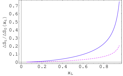
Figure 2: $\Delta S_{t}/S_{0}(x_{t})$ versus $x_{L}$ for different values of f, $f=1$ TeV (solid) and $f=2$ TeV (dashed). $\mathcal{O}(v^{4}/f^{4})$ corrections are included to show the large $x_{L}$ behavior.

The leading order $\mathcal{O}(v^{2}/f^{2})$ contribution to the effective Hamiltonian that governs $K$ meson mixing from the T-even sector is given by

$$\mathcal{H}_{\mathrm{eff}}^{\rm even}=\frac{G_{F}^{2}}{16\pi^{2}}M_{W}^{2}\left[\lambda_{c}^{2}\eta_{1}\Delta S_{c}+\lambda_{t}^{2}\eta_{2}\Delta S_{t}+2\lambda_{c}\lambda_{t}\eta_{3}\Delta S_{tc}\right](\bar{s}d)_{V_{A}}(\bar{s}d)_{V-A},$$ (5.51)

where

$$\Delta S_{c}=0$$

$$\Delta S_{t}=-2\frac{v^{2}}{f^{2}}x_{L}^{2}\Big{(}S_{0}(x_{t})-S_{0}(x_{t},x_{T})\Big{)}$$

$$\Delta S_{ct}=-\frac{v^{2}}{f^{2}}x_{L}^{2}\Big{(}S_{0}(x_{c},x_{t})-S_{0}(x_{c},x_{T})\Big{)},$$ (5.52)

and $x_{T}=m_{T_{+}}^{2}/m_{W_{L}}^{2}$. The parameter $x_{L}$ is a function of the couplings in Eq. (2.21):

$$x_{L}=\frac{\lambda_{1}^{2}}{\lambda_{1}^{2}+\lambda_{2}^{2}}.$$ (5.53)

These corrections arise from two effects. First, there are explicit new flavor changing diagrams which involve the partner of the top quark, $T_{+}$. In addition, the CKM matrix is modified at order $v^{2}/f^{2}$ in the $V_{\rm CKM}^{ti}$ elements.

To obtain these relations, we have simply taken the limit of equal gauge couplings required by T-parity in the equations in [19], and removed also the contributions from diagrams that violate T-parity. Note that, because of those new conditions, imposing T-parity makes the T-even contributions somewhat smaller than those in the littlest Higgs model without T-parity.

For regions of $x_{L}\geq 0.8$, where $\lambda_{1}>\lambda_{2}$, we have to also consider formally order $v^{4}/f^{4}$ contributions, which increase linearly with $x_{T}$. These contributions come from box diagrams that contain two T-even partners of the top quark. The leading behavior of these contributions is the same as that of the littlest Higgs model without T-parity, given by [19]

$$(\Delta S_{t})_{TT}\approx\frac{x_{T}}{4}\frac{v^{4}}{f^{4}}\,x_{L}^{4}=\frac{x_{t}}{4}\frac{v^{2}}{f^{2}}\frac{x_{L}^{3}}{1-x_{L}}.$$ (5.54)

In Figure 2, we show the ratio $\Delta S_{t}/S_{0}(x_{t})$ as a function of $x_{L}$ at order $\mathcal{O}(v^{4}/f^{4})$, where $S_{0}$ is the SM contribution. In our analysis, we take $x_{L}=0.5$, which corresponds to the point at which the $T_{+}$ mass is at its minimum. This is also the point where the contributions to the Higgs mass are minimized. For this ‘natural’ value of $x_{L}$, these T-even contributions are small (less than $6$% of the SM contribution for $f=1$ TeV), and can be neglected.

Although T-even contributions could be very large in more fine-tuned regions of $x_{L}$, we note that $x_{L}$ cannot be arbitrarily close to 1, in order not to violate direct search bounds on the T-odd top partner mass, $m_{T_{-}}=\lambda_{2}f$ (as $\lambda_{1}$ is increased, in order to hold the top quark mass fixed, $\lambda_{2}$ must decrease, lowering the $T_{-}$ mass). In addition, we want to keep $\lambda_{1}$ from entering the strong coupling regime. We leave a study which includes the effects of large $x_{L}$ for future work.

5.3 QCD corrections

So far the expressions we have presented did not include QCD corrections. For the SM contributions these corrections usually suppress the short distance predictions. For example, the numerical values for the QCD corrections to the SM contributions are given by

$$\eta_{B}=0.55\pm 0.01,\ \eta_{1}=1.32\pm 0.32,\ \eta_{2}=0.57\pm 0.01,\ \eta_{3}=0.47\pm 0.05$$ (5.55)

at NLO [29, 35, 36, 37, 38]. A full NLO analysis for the new physics contributions would clearly be beyond the scope of this work, but as we will show below, we can account for the bulk of these corrections at leading order (LO).

For the little Higgs model with T-parity we always match onto the same $(V-A)\otimes(V-A)$ operator. While the NLO value of the Wilson coefficient at the high scale $\mu_{H}$ cannot be determined without a full one loop calculation, the anomalous dimension will be the same as in the SM, as it depends only on the properties of the local operator. This implies that we can immediately obtain $\eta=\alpha_{s}(\mu_{H})^{\frac{\gamma_{0}}{2\beta_{0}}}$, valid at LO.

We also need to address the issue of the choice of what to take for the high scale $\mu_{H}$. One might assume that $\mu_{H}\sim f$ is the best choice, but as we will explain below, we choose for our study $\mu_{H}\sim M_{W}$.

• While the masses of $W_{H}$ and $Z_{H}$ are $gf$, the mass of $A_{H}$ is $4$ times smaller: $g\,^{\prime}f/\sqrt{5}$, which for $f\sim$ 1000 GeV is close to the top quark mass. Therefore for diagrams that involve $A_{H}$ we should use a scale lower than $f$.

• The masses of the T-odd fermions are free parameters, so it is unclear which scale to use when integrating them out. Furthermore, since they couple to the gluons, their presence will lead to threshold effects which are functions of these masses and which greatly complicate the calculation.

• Most importantly, the bulk of the QCD corrections result from running from the weak scale to the hadronic scale. Since the variation of $\alpha_{s}$ between the scales $v$ and $f$ is rather small, neglecting these running and threshold effects is justified, considering the other uncertainties. For example, in running up to $f=1000$ GeV from $M_{W}$, the effect would only reduce $\eta$ by about $8\%$.

Considering these facts, and that there are uncertainties which would dominate these small effects, the common value for the QCD corrections that we adopt is then:

$$\eta=(\alpha_{s}(m_{W_{L}}))^{\frac{\gamma_{0}}{2\beta_{0}}}=(\alpha_{s}(m_{W_{L}}))^{6/23}\sim 0.58\ .$$ (5.56)

In order to calculate the matrix element of the resulting effective Hamiltonian, we need to parametrize the matrix element of the four quark operator. This calculation is precisely the same as in the SM as it only relies on physics at the low scale, and so the bag parameters are identical.

6 Results and Constraints

In this section, we show our numerical bounds on the T-odd fermion spectrum for some representative selection of textures for $V_{Hd}$. We first consider cases where $V_{Hu}$ and $V_{Hd}$ are diagonal up to corrections that are of order the off-diagonal elements of $V_{{\rm CKM}}$. We then analyze simple cases where the off-diagonal elements are allowed to be large. We find in the former cases that some small GIM suppression is necessary to satisfy experimental constraints. In the large mixing scenarios, a strong GIM suppression is necessary to avoid large contributions, and the T-odd fermion spectrum must be nearly degenerate.

6.1 Near the diagonal

The littlest Higgs model is an effective field theory valid at most to the scale $4\pi f$. As such, there is no reason to suspect that one particular texture is favored over another. However, if we begin from a basis where the T-odd Dirac masses are diagonal, this leads to the relations $V_{Hu}=V_{u}$, and $V_{Hd}=V_{d}$. From this relation, it is clear that, in this basis, all of the flavor and CP violating amplitudes arise as a result of the Yukawa couplings which give mass to the SM fermions.

Now the CKM matrix is given by $V_{{\rm CKM}}=V_{u}^{\dagger}V_{d}$. From this relation, it is clear that $V_{u}$ and $V_{d}$ cannot simultaneously be set to the identity. In this section, we assume that both $V_{u}$ and $V_{d}$ are nearly equal to the identity matrix. This is equivalent to assuming that there is an alignment mechanism between the T-odd masses and the SM Yukawa structure. This assumption provides us with a set of minimal mixing scenarios. We take as examples two simple cases:

• Case I     $V_{Hu}={\mathbf{1}}$, $V_{Hd}=V_{{\rm CKM}}$

• Case II   $V_{Hd}={\mathbf{1}}$, $V_{Hu}=V_{{\rm CKM}}^{\dagger}$

In each of these scenarios, the only parameters relevant to neutral meson mixing are the mass eigenvalues of the T-odd fermions. In the first setup, the $D$ system is unaffected, and all constraints arise from neutral $K$ and $B$ mixing. In the second, there is no mixing in the down type gauge and Goldstone boson interactions, and thus there are no contributions at one loop order in the $K$ and $B$ systems. Instead, the $D$ system gives the only constraints.

The one feature that these scenarios both share is a relative suppression mechanism that is borrowed from the SM CKM texture. The smallness of $V^{ub}_{{\rm CKM}}$ and $V^{td}_{{\rm CKM}}$ ensure that the neutral meson mixing amplitudes will be nearly independent of the mass of the third generation T-odd fermions. The constraints will primarily be on the masses of the first two generations of T-odd fermions, because of the relatively larger values of $V^{us}_{{\rm CKM}}$ and $V^{cd}_{{\rm CKM}}$.

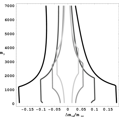
Figure 3: Case I $f=1000$ GeV: In these plots, $V_{Hd}=V_{{\rm CKM}}$. In order of the darkest contours to lightest, the average mass of the first two generations varies through $m_{12}=500,1000,2000,3000\ {\rm GeV}$. The $D$ system imposes no constraints in this scenario.

In finding the bounds on the mass eigenvalues of the T-odd fermion sector for a particular texture, we require that, for $B_{d}$ and $K$ mixing, the contribution from the T-odd fermions not exceed $30\%$ of the SM contribution to the mass splittings and $\epsilon_{K}$. This is roughly when the new physics contributions begin to exceed the long distance uncertainties associated with the SM predictions for these observables. We note that this process eliminates the dependance on the bag parameters, which have rather large theoretical uncertainties. In the $D$ system, there is only an experimental upper bound on the mass splitting, and the SM short distance contribution is very small compared with this bound. Thus, for the $D$ system we only require that the T-odd fermion contributions not exceed this experimental upper bound. For every scenario, we hold the symmetry breaking scale $f$ fixed at $f=1000$ GeV. The contributions from new physics simply scale as $1/f^{2}$, so these results can easily be extended to other values of the breaking scale. In each plot, the horizontal axis is the ratio $\Delta m_{12}/m_{12}=2(m_{2}-m_{1})/(m_{1}+m_{2})$, where $m_{12}$ is the average mass of the first two generations, and $\Delta m_{12}$ is the splitting $m_{2}-m_{1}$. On the vertical axes we plot the dependence on the mass of the third generation T-odd quark doublet.

In Figure 3, we show the constraints on the mass splitting of the first two generations of T-odd fermions as a function of the mass of the third generation T-odd doublet. The regions of parameter space where the new physics contributions are smaller than the approximate long distance uncertainties in the SM contributions lie inside the shown contours. In this scenario the up-type CKM, $V_{Hu}$, is diagonal, and thus $D^{0}-\bar{D}^{0}$ mixing has no contributions from new physics. The features in the plot that cause the narrowing of the internal regions as $m_{3}$ varies away from $m_{12}$ are due to the influence of the $\epsilon_{K}$ observable. If the CP violating phase $\delta_{13}^{d}$ is set to zero, the contours are nearly vertical.

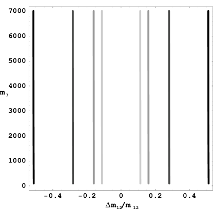
Figure 4: Case II $f=1000$ GeV: In this plot, we show the results for the case where $V_{Hd}={\mathbf{1}}$. Again, from darkest to lightest, the average mass of the first two generations increases as $m_{12}=500,1000,2000,3000\ {\rm GeV}$. In this scenario, only the $D$ system is affected, and so the contours correspond to the points at which the T-odd fermion contributions exceed the experimental upper bounds.

In Figure 4, we set instead the down-type Yukawa interactions to be diagonal. As mentioned, the constraints in this region come only from the $D$ system mass splitting. There are essentially no constraints on the mass of the third generation T-odd doublet. The degeneracy required in the first two generations is quite relaxed, now varying between $50$ and $10$% as the average mass $m_{12}$ is increased. We note, however, that this would change as the experimental bounds on the $D$ meson mass splitting are improved. For example, if the bound on the mass splitting comes down by a factor of ten, the required degeneracy between the first two generations of T-odd fermions then varies between about $16$ and $4$% as $m_{12}$ varies between $500$ and $3000$ GeV.

6.2 Going away from the diagonal

As mentioned, another possibility for the textures is to have large off diagonal elements in $V_{Hd}$. There is no reason to assume that there is an alignment between the T-odd mass textures and the SM Yukawa couplings. We note that this requires that there are also, simultaneously, large off diagonal elements in $V_{Hu}$ which must cancel in the relation $V_{Hu}^{\dagger}V_{Hd}=V_{u}^{\dagger}V_{H}V_{H}^{\dagger}V_{d}=V_{{\rm CKM}}$. This is easy to realize in a natural way if most of this mixing comes in through the T-odd Yukawa textures.

In this section, we study the corrections that arise when the angles $s_{ij}^{d}$ in Eq. (3.34) are taken to be large. In these cases, we find that not only is a degeneracy required between the first two generations, but the entire flavor spectrum of the T-odd vector-like quarks must often be degenerate. We consider four scenarios:

• Case IIIa $s_{13}^{d}=0.5$, $\delta_{13}^{d}=\delta_{13}^{SM}$, $s_{ij}^{d}=s_{ij}^{SM}$ otherwise.

• Case IIIb $s_{13}^{d}=0.5$, $\delta_{13}^{d}=0$, $s_{ij}^{d}=s_{ij}^{SM}$ otherwise

• Case IVa $s_{13}^{d}=0.5$, $s_{12}^{d}=0.7$, $s_{23}^{d}=0.4$, $\delta_{13}^{d}=\delta_{13}^{SM}$

• Case IVb $s_{13}^{d}=0.5$, $s_{12}^{d}=0.7$, $s_{23}^{d}=0.4$, $\delta_{13}^{d}=0$

In cases IIIa and IIIb, we allow one of the angles to be large. We pick specifically $s_{13}^{d}$ to be large, as it is this angle to which the third generation mass dependence is sensitive. As $\epsilon_{K}$ is a strong factor in the analysis, we look at the case where it receives no contributions by setting $\delta_{13}^{d}$ to zero, relegating all new CP violation to the up-type quark interactions. In cases Va and Vb, we chose some order one values for the three mixing angles, and again look at cases where the new CP violating phase is either all in the down-type, or all in the up-type quark interactions.

 

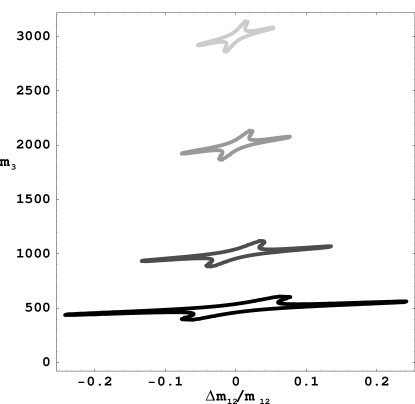
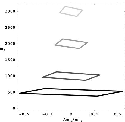
Figure 5: Case III $f=1000$ GeV: In this plot, the angle $s_{13}^{d}=0.5$, while the other angles are equal to the SM CKM angles. The contributions from new physics are generally much larger, and thus a stronger GIM suppression is necessary. The contours, from darkest to lightest, are for $m_{12}=500,1000,2000,3000$ GeV. In the plot on the left, $\delta_{13}^{d}=\delta_{13}^{SM}=1.05$, while on the right this phase is set to zero.

In Figure 5, we show the constraints on the masses in this case where $s_{13}^{d}$ is large. A large $s_{13}^{d}$ implies order one contributions to $V_{Hd}^{3d}$ and $V_{Hd}^{1b}$. It is clear from this figure that a degeneracy is now required in all three generations of T-odd fermions. For a generic choice of order one mixing angles, it is expected that such a universally degenerate spectrum is required. We show the results when the CP violating phase is set both to the SM value, $\delta_{13}^{d}=1.05$, and to $\delta_{13}^{d}=0$. The dramatic difference between these two types of scenarios indicates the severe sensitivity of the $\epsilon_{K}$ observable to new flavor physics.

In Figure 6, we take all of the mixing angles to be somewhat large. We find that this scenario is far more constrained then all the others if the phase $\delta_{13}^{d}=\delta_{13}^{SM}$. There are some narrow windows where degeneracies of up to $10$% are allowed, but the majority of the parameter space where corrections are small is in the $1$% range. However, when the angle $\delta_{13}^{d}$ is taken to be small, it happens that there is a cancellation in $V_{Hd}^{3d}$, such that the third generation mass $m_{3}$ is relatively unconstrained.

 

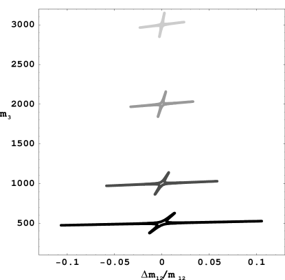
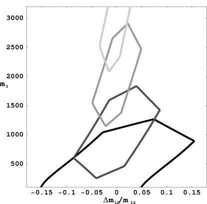
Figure 6: Case IV $f=1000$ GeV: In this plot, all of the angles are taken to be somewhat large: $s_{12}^{d}=0.5,\ s_{13}^{d}=0.7,\ s_{23}^{d}=0.4$. The contours, from darkest to lightest, are for $m_{12}=500,1000,2000,3000$ GeV. In the plot on the left, $\delta_{13}^{d}=\delta_{13}^{SM}=1.05$, while on the right this phase is set to zero. In the plot on the right, the required degeneracy in the third generation is relaxed.

6.3 $B_{s}$ mixing

Of all the scenarios that we have considered so far, $B_{s}$ mixing is not strongly affected if the T-odd fermion spectrum is constrained such that the new physics contributions to $K$, $B_{d}$, and $D$ mixing do not exceed the bounds that we impose. However, there may be some special choices of textures that we have not considered that only strongly modify the $B_{s}$ system. It is well known that this can occur in supersymmetry [13]. With this in mind, we have identified a texture that does not significantly affect $K$ and $B_{d}$ mixing, but which is able to enhance $B_{s}$ mixing. A simple set of angles that achieves this is

• Case V $s_{23}^{d}=1/\sqrt{2}$, $s_{12}^{d}=0$, $s_{13}^{d}=0$, $\delta_{13}^{d}=0$.

The constraints from the other neutral meson systems are very weak here. It is primarily the $D$ system which restricts the allowed parameter space. In this scenario, by varying the T-odd fermion masses within the allowed contours, the mass splitting in the $B_{s}$ system can be enhanced by as much as a factor of $12$. The constraints, along with a plot where we show the enhancement of the $B_{s}$ mass splitting for fixed $m_{12}=3000$ GeV are shown in Figure 7. It is interesting to note that the degeneracy required in the first two generations of T-odd fermions is more or less completely relaxed. We emphasize that we have not performed an exhaustive search, and it is possible that there are other textures where the allowed enhancement of $B_{s}$ mixing is even larger.

 

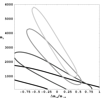
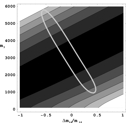
Figure 7: Case V $f=1000$ GeV: In these plots, the angle $s_{23}^{d}=1/\sqrt{2}$, while the other angles are set to zero. In the plot on the left, the contours, from darkest to lightest, are for $m_{12}=500,1000,2000,3000$ GeV, and show the constraints from the $K$, $B_{d}$, and $D$ systems. In the plot on the right, we overlap the constraint contour for $m_{12}=3000$ GeV with a plot of the enhancement in the $B_{s}$ mass splitting relative to the SM contribution. From darkest to lightest, this enhancement is a factor of $2,4,6,8,10,$ and $12$, respectively.

7 Conclusions

Little Higgs models with T-parity necessarily introduce new mirror fermions in order to cut off UV sensitive contributions to four-fermion contact operators that are constrained primarily by studies at LEP. These fermions introduce a new flavor structure to the model, and lead to new tree level flavor changing currents involving SM fermions and mirror fermions. We have done a first exploratory study of this flavor structure, and found constraints on the mirror fermion mass spectrum from a one loop analysis of neutral meson mixing. We have noted that it is not possible to adjust all of the new flavor structure to be completely diagonal, due to relations with the CKM mixing already present in the SM.

For order one mixing parameters, we find that the mirror fermion mass spectrum must be degenerate to within a few percent or less. If the new mixing parameters are taken to be small, then this is significantly relaxed. In particular, if all mixing is relegated to the up-type quark interactions, only $D$ mixing is affected, and a degeneracy of only $50$% or so is required between the first two generations of T-odd fermions. We note that improved experimental constraints on the $D$ meson mass splitting could significantly restrict such scenarios. We have found that the $\epsilon_{K}$ observable plays a significant role in the fits if there is a CP violating phase in $V_{Hd}$.

We have also studied the $B_{s}$ system, identifying a scenario in which $B^{0}_{s}-\bar{B}^{0}_{s}$ mixing can differ substantially from the SM prediction while still satisfying constraints on the other neutral meson mixing observables. In the setup we have considered, the enhancement of the mass splitting can be as large as a factor of $12$. Such scenarios are of particular interest for experimental studies of the $B_{s}$ system. Also, in this scenario, the constraints on the first two generations are much more relaxed than in the others considered.

We wish to make clear that little Higgs models with T-parity are not ruled out in any way by this study. This analysis should instead serve as a guide to what properties any UV completion of this structure should have. This is in close analogy with studies of the supersymmetric flavor problem, which have been an essential tool in constructing mechanisms of supersymmetry breaking which are consistent with low energy phenomenology.

We note that this is only an introduction to the flavor physics of this model. There are many other observables which are sensitive to this flavor structure, such as rare decays and lepton flavor violating processes. Including rare decay processes in an analysis would possibly require a closer degeneracy in the mass spectrum, although this needs to be checked. In addition, we have assumed that the SM CKM fit is unchanged, when in fact additional contributions to observables (especially $\epsilon_{K}$) can change the best fit values of the CKM elements. A full global analysis would remedy this situation, however many more observables must be computed and included to render such a fit meaningful.

Appendix

The gauge and Yukawa interactions of the littlest Higgs model with T-parity lead to tree level flavor changing currents which can, at one loop, affect SM observables such as neutral meson mixing. After identifying the mass eigenstates, the Lagrangian can be expanded, leading to the relevant Feynman rules. These rules are given in Table 1. While the conjugate interactions are not shown explicitly, they are easily derived. One should note that the Yukawa type interactions with the eaten Goldstone bosons do not have an $i$ prefactor. Because of this, the associated conjugate Feynman rules have an additional minus sign.

Particles	Vertices	Particles	Vertices
$\bar{u}_{Hi}W_{H}^{+\mu}d^{j}$	$i\frac{g}{\sqrt{2}}(V_{Hd})^{i}_{j}\gamma^{\mu}P_{L}$	$\bar{d}_{Hi}W_{H}^{-\mu}u^{j}$	$i\frac{g}{\sqrt{2}}(V_{Hu})^{i}_{j}\gamma^{\mu}P_{L}$
$\bar{u}_{Hi}Z_{H}^{\mu}u^{j}$	$i\frac{g}{2}(V_{Hu})^{i}_{j}\gamma^{\mu}P_{L}$	$\bar{d}_{Hi}Z_{H}^{\mu}d^{j}$	$-i\frac{g}{2}(V_{Hd})^{i}_{j}\gamma^{\mu}P_{L}$
$\bar{u}_{Hi}A_{H}^{\mu}u^{j}$	$-i\frac{g^{\prime}}{10}(V_{Hu})^{i}_{j}\gamma^{\mu}P_{L}$	$\bar{d}_{Hi}A_{H}^{\mu}d^{j}$	$-i\frac{g^{\prime}}{10}(V_{Hd})^{i}_{j}\gamma^{\mu}P_{L}$
$\bar{u}_{Hi}d^{j}\omega^{+}$	$-\frac{1}{\sqrt{2}f}M_{u_{H}^{i}}(V_{Hd})^{i}_{j}P_{L}$	$\bar{d}_{Hi}u^{j}\omega^{-}$	$-\frac{1}{\sqrt{2}f}M_{d_{H}^{i}}(V_{Hu})^{i}_{j}P_{L}$
$\bar{u}_{Hi}u^{j}w_{3}$	$-\frac{1}{2f}M_{u_{H}^{i}}(V_{Hu})^{i}_{j}P_{L}$	$\bar{d}_{Hi}\omega_{3}d^{j}$	$\frac{1}{2f}M_{d_{H}^{i}}(V_{Hd})^{i}_{j}P_{L}$
$\bar{u}_{Hi}u^{j}\eta$	$\frac{1}{\sqrt{20}f}M_{u_{H}^{i}}(V_{Hu})^{i}_{j}P_{L}$	$\bar{d}_{Hi}d^{j}\eta$	$\frac{1}{\sqrt{20}f}M_{d_{H}^{i}}(V_{Hd})^{i}_{j}P_{L}$
$\bar{\nu}_{Hi}W_{H}^{+\mu}e^{j}$	$i\frac{g}{\sqrt{2}}(V_{He})^{i}_{j}\gamma^{\mu}P_{L}$	$\bar{e}_{Hi}W_{H}^{-\mu}\nu^{j}$	$i\frac{g}{\sqrt{2}}(V_{H\nu})^{i}_{j}\gamma^{\mu}P_{L}$
$\bar{\nu}_{Hi}Z_{H}^{\mu}\nu^{j}$	$i\frac{g}{2}(V_{H\nu})^{i}_{j}\gamma^{\mu}P_{L}$	$\bar{e}_{Hi}Z_{H}^{\mu}e^{j}$	$-i\frac{g}{2}(V_{He})^{i}_{j}\gamma^{\mu}P_{L}$
$\bar{\nu}_{Hi}A_{H}^{\mu}\nu^{j}$	$i\frac{g^{\prime}}{10}(V_{H\nu})^{i}_{j}\gamma^{\mu}P_{L}$	$\bar{e}_{Hi}A_{H}^{\mu}e^{j}$	$i\frac{g^{\prime}}{10}(V_{He})^{i}_{j}\gamma^{\mu}P_{L}$
$\bar{\nu}_{Hi}e^{j}\omega^{+}$	$-\frac{1}{\sqrt{2}f}M_{\nu_{H}^{i}}(V_{He})^{i}_{j}P_{L}$	$\bar{e}_{Hi}\nu^{j}\omega^{-}$	$-\frac{1}{\sqrt{2}f}M_{e_{H}^{i}}(V_{H\nu})^{i}_{j}P_{L}$
$\bar{\nu}_{Hi}\nu^{j}w_{3}$	$-\frac{1}{2f}M_{\nu_{H}^{i}}(V_{H\nu})^{i}_{j}P_{L}$	$\bar{e}_{Hi}\omega_{3}e^{j}$	$\frac{1}{2f}M_{e_{H}^{i}}(V_{He})^{i}_{j}P_{L}$
$\bar{\nu}_{Hi}\nu^{j}\eta$	$\frac{1}{\sqrt{20}f}M_{\nu_{H}^{i}}(V_{H\nu})^{i}_{j}P_{L}$	$\bar{e}_{Hi}e^{j}\eta$	$\frac{1}{\sqrt{20}f}M_{e_{H}^{i}}(V_{He})^{i}_{j}P_{L}$

Table 1: This table contains the Feynman rules relevant to flavor changing physics. The conjugate interactions are not included, but can easily be derived from the listed expressions.

The functions resulting from evaluation of the box diagrams are given by

$$F(y_{i},y_{j};W_{H})=\frac{1}{(1-y_{i})(1-y_{j})}\left(1-\frac{7}{4}y_{i}y_{j}\right)+\frac{y_{i}^{2}\log y_{i}}{(y_{i}-y_{j})(1-y_{i})^{2}}\left(1-2y_{j}+\frac{y_{i}y_{j}}{4}\right)$$

$$\hskip 242.10493pt-\frac{y_{j}^{2}\log y_{j}}{(y_{i}-y_{j})(1-y_{j})^{2}}\left(1-2y_{i}+\frac{y_{i}y_{j}}{4}\right)$$

$$G(z_{i},z_{j};Z_{H})=-\frac{3}{4}\left[\frac{1}{(1-z_{i})(1-z_{j})}+\frac{z_{i}^{2}\log z_{i}}{(z_{i}-z_{j})(1-z_{i})^{2}}-\frac{z_{j}^{2}\log z_{j}}{(z_{i}-z_{j})(1-z_{j})^{2}}\right]$$

$$A_{1}(z_{i},z_{j};Z_{H})=-\frac{3}{100a}\left[\frac{1}{(1-z^{\prime}_{i})(1-z^{\prime}_{j})}+\frac{z^{\prime}_{i}z_{i}\log z^{\prime}_{i}}{(z_{i}-z_{j})(1-z^{\prime}_{i})^{2}}-\frac{z^{\prime}_{j}z_{j}\log z^{\prime}_{j}}{(z_{i}-z_{j})(1-z^{\prime}_{j})^{2}}\right]$$

$$A_{2}(z_{i},z_{j};Z_{H})=-\frac{3}{10}\left[\frac{\log a}{(a-1)(1-z^{\prime}_{i})(1-z^{\prime}_{j})}+\frac{z_{i}^{2}\log z_{i}}{(z_{i}-z_{j})(1-z_{i})(1-z^{\prime}_{i})}\right.$$

$$\hskip 234.87749pt\left.-\frac{z_{j}^{2}\log z_{j}}{(z_{i}-z_{j})(1-z_{j})(1-z^{\prime}_{j})}\right],$$

(7.57)

where $a=M_{Z_{H}}^{2}/M_{A_{H}}^{2}\approx 5/\tan^{2}\theta_{w}$, and $z^{\prime}_{i}=az_{i}$. The function $F$ contains the contributions from the charged T-odd scalars and gauge bosons, while $G$ contains the contributions involving two $Z_{H}$ propagators. $A_{1}$ contains the contributions from diagrams with two $A_{H}$ propagators, while $A_{2}$ contains the contributions from diagrams with both a $Z_{H}$ and an $A_{H}$ propagator running in the loop.

We note that in unitary gauge the expression for the $F$ function is not the same, and in fact contains divergent terms. These cancel when the sum over flavors running in the box diagrams is performed, and unitarity of the mixing matrices is imposed. It is only after this summation that the calculations in the two different gauges can be compared. In contrast, the $G$, $A_{1}$, and $A_{2}$ functions which correspond to neutral current contributions are already gauge invariant.

References

- [1]
- [2] N. Arkani-Hamed, A. G. Cohen and H. Georgi, Phys. Rev. Lett. 86, 4757 (2001) [arXiv:hep-th/0104005]. N. Arkani-Hamed, A. G. Cohen and H. Georgi, Phys. Lett. B 513, 232 (2001) [hep-ph/0105239].
- [3] For a recent review and a comprehensive collection of references, see M. Schmaltz and D. Tucker-Smith, arXiv:hep-ph/0502182.
- [4] H. Georgi and A. Pais, Phys. Rev. D 10, 539 (1974); Phys. Rev. D 12, 508 (1975).
- [5] D. B. Kaplan and H. Georgi, Phys. Lett. B 136, 183 (1984); Phys. Lett. B 145, 216 (1984); D. B. Kaplan, H. Georgi and S. Dimopoulos, Phys. Lett. B 136, 187 (1984); H. Georgi, D. B. Kaplan and P. Galison, Phys. Lett. B 143, 152 (1984); M. J. Dugan, H. Georgi and D. B. Kaplan, Nucl. Phys. B 254, 299 (1985).
- [6] N. Arkani-Hamed, A. G. Cohen, E. Katz and A. E. Nelson, JHEP 0207, 034 (2002) [arXiv:hep-ph/0206021].
- [7] C. Csaki, J. Hubisz, G. D. Kribs, P. Meade and J. Terning, Phys. Rev. D 67, 115002 (2003) [arXiv:hep-ph/0211124]; J. L. Hewett, F. J. Petriello and T. G. Rizzo, JHEP 0310, 062 (2003) [arXiv:hep-ph/0211218]. C. Csaki, J. Hubisz, G. D. Kribs, P. Meade and J. Terning, Phys. Rev. D 68, 035009 (2003) [arXiv:hep-ph/0303236]. M. C. Chen and S. Dawson, Phys. Rev. D 70, 015003 (2004) [arXiv:hep-ph/0311032].
- [8] H. C. Cheng and I. Low, JHEP 0309, 051 (2003) [arXiv:hep-ph/0308199]; JHEP 0408, 061 (2004) [arXiv:hep-ph/0405243].
- [9] I. Low, JHEP 0410, 067 (2004) [arXiv:hep-ph/0409025].
- [10] K. m. Cheung, Phys. Lett. B 517, 167 (2001) [arXiv:hep-ph/0106251].
- [11] F. Gabbiani, E. Gabrielli, A. Masiero and L. Silvestrini, Nucl. Phys. B 477, 321 (1996) [arXiv:hep-ph/9604387].
- [12] S. L. Glashow, J. Iliopoulos and L. Maiani, Phys. Rev. D 2, 1285 (1970).
- [13] Y. Grossman, M. Neubert and A. L. Kagan, JHEP 9910, 029 (1999) [arXiv:hep-ph/9909297].
- [14] Y. Nir, arXiv:hep-ph/0510413.
- [15] S. R. Coleman, J. Wess and B. Zumino, “Structure Of Phenomenological Lagrangians. 1,” Phys. Rev. 177, 2239 (1969). C. G. . Callan, S. R. Coleman, J. Wess and B. Zumino, “Structure Of Phenomenological Lagrangians. 2,” Phys. Rev. 177, 2247 (1969).
- [16] J. Hubisz, P. Meade, A. Noble and M. Perelstein, arXiv:hep-ph/0506042.
- [17] J. Hubisz and P. Meade, Phys. Rev. D 71, 035016 (2005) [arXiv:hep-ph/0411264].
- [18] N. Cabibbo, Phys. Rev. Lett. 10, 531 (1963). M. Kobayashi and T. Maskawa, Prog. Theor. Phys. 49, 652 (1973).
- [19] A. J. Buras, A. Poschenrieder and S. Uhlig, Nucl. Phys. B 716, 173 (2005) [arXiv:hep-ph/0410309]; arXiv:hep-ph/0501230.
- [20] G. Burdman, M. Perelstein and A. Pierce, “Collider tests of the little Higgs model,” Phys. Rev. Lett. 90, 241802 (2003) [Erratum-ibid. 92, 049903 (2004)] [arXiv:hep-ph/0212228].
- [21] T. Han, H. E. Logan, B. McElrath and L. T. Wang, Phys. Rev. D 67, 095004 (2003) [arXiv:hep-ph/0301040].
- [22] M. Perelstein, M. E. Peskin and A. Pierce, “Top quarks and electroweak symmetry breaking in little Higgs models,” Phys. Rev. D 69, 075002 (2004) [arXiv:hep-ph/0310039].
- [23] G. Azuelos et al., Eur. Phys. J. C 39S2, 13 (2005) [arXiv:hep-ph/0402037].
- [24] S. Eidelman et al. [Particle Data Group], Phys. Lett. B 592, 1 (2004).
- [25] G. Buchalla, A. J. Buras and M. E. Lautenbacher, Rev. Mod. Phys. 68, 1125 (1996) [arXiv:hep-ph/9512380].
- [26] A. J. Buras, arXiv:hep-ph/0101336.
- [27] M. Battaglia et al., arXiv:hep-ph/0304132.
- [28] A. J. Buras, Lect. Notes Phys. 629, 85 (2004) [arXiv:hep-ph/0307203].
- [29] A. J. Buras, arXiv:hep-ph/0505175.
- [30] T. Inami and C. S. Lim, Prog. Theor. Phys. 65, 297 (1981) [Erratum-ibid. 65, 1772 (1981)].
- [31] D. Y. Bardin and G. Passarino, The standard model in the making: Precision study of the electroweak interactions, (Oxford University Press, USA, 1999)
- [32] S. R. Choudhury, N. Gaur, A. Goyal and N. Mahajan, Phys. Lett. B 601, 164 (2004) [arXiv:hep-ph/0407050].
- [33] J. Y. Lee, JHEP 0412, 065 (2004) [arXiv:hep-ph/0408362].
- [34] H. C. Cheng, I. Low and L. T. Wang, arXiv:hep-ph/0510225.
- [35] A. J. Buras, M. Jamin and P. H. Weisz, Nucl. Phys. B 347, 491 (1990).
- [36] S. Herrlich and U. Nierste, Nucl. Phys. B 419, 292 (1994) [arXiv:hep-ph/9310311].
- [37] S. Herrlich and U. Nierste, Nucl. Phys. B 476, 27 (1996) [arXiv:hep-ph/9604330].
- [38] S. Herrlich and U. Nierste, Phys. Rev. D 52, 6505 (1995) [arXiv:hep-ph/9507262].
- [39]