Discovery Limits for Techni-Omega Production in $e\gamma$ Collisions

Abstract

In a strongly-interacting electroweak sector with an isosinglet vector state, such as the techni-omega, $\omega_{T}$, the direct $\omega_{T}Z\gamma$ coupling implies that an $\omega_{T}$ can be produced by $Z\gamma$ fusion in $e\gamma$ collisions. This is a unique feature for high energy $e^{+}e^{-}$ or $e^{-}e^{-}$ colliders operating in an $e\gamma$ mode. We consider the processes $e^{-}\gamma\to e^{-}Z\gamma$ and $e^{-}\gamma\to e^{-}W^{+}W^{-}Z$, both of which proceed via an intermediate $\omega_{T}$. We find that at a 1.5 TeV $e^{+}e^{-}$ linear collider operating in an $e\gamma$ mode with an integrated luminosity of 200 fb^-1, an $\omega_{T}$ can be discovered for a broad range of masses and widths.

I Introduction

The mechanism for electroweak symmetry breaking remains the most prominent mystery in elementary particle physics. In the Standard Model (SM), a neutral scalar fundamental Higgs boson is expected with a mass ($m_{H}$) less than about 800 GeV. In the weakly coupled supersymmetric extension of the SM, the lightest Higgs boson is expected to be lighter than about 140 GeV. Searching for the Higgs bosons is a primary goal of current and future collider experiments [1]. However, if no light fundamental Higgs boson is found for $m_{H}<800$ GeV, one would anticipate that the interactions among the longitudinal vector bosons become strong [2]. This is the case when strongly interacting dynamics is responsible for electroweak symmetry breaking, such as in Technicolor models [3].

Without knowing the underlying dynamics of the strongly-interacting electroweak sector (SEWS), it is instructive to parametrize the physics with an effective theory for the possible low-lying resonant states. This typically includes an isosinglet scalar meson $(H)$ and an isotriplet vector meson $(\rho_{T})$ [4]. However, in many dynamical electroweak symmetry breaking models there exist other resonant states such as an isosinglet vector ($\omega_{T}$), and isotriplet vector ($a_{1_{T}}$) [5, 6]. In fact it has been argued that to preserve good high energy behavior for strong scattering amplitudes in a SEWS, it is necessary for all the above resonant states to coexist [7]. It is therefore wise to keep an open mind and to consider other characteristic resonant states when studying the physics of a SEWS at high energy colliders.

Among those heavy resonant states, the isosinglet vector state $\omega_{T}$ has rather unique features. Due to its isosinglet nature, it does not have strong coupling to two gauge bosons. It couples strongly to three longitudinal gauge bosons $W^{+}_{L}W^{-}_{L}Z_{L}$ (or equivalently, electroweak Goldstone bosons $w^{+}w^{-}z$) and electroweakly to $Z\gamma$, $ZZ$, and $W^{+}W^{-}$. It may mix with the $U(1)$ gauge boson $B$, depending on its hypercharge assignment in the model. The signal for $\omega_{T}$ production was studied for $pp$ collisions at 40 TeV and 17 TeV [5, 6]. It appears to be difficult to observe the $\omega_{T}$ signal at the LHC, largely due to the SM backgrounds. On the other hand, the direct $\omega_{T}Z_{L}\gamma$ coupling implies that an $\omega_{T}$ can be effectively produced by $Z_{L}\gamma$ fusion in $e\gamma$ collisions. This is a unique feature for high energy $e^{+}e^{-}$ or $e^{-}e^{-}$ colliders operating in an $e\gamma$ mode. In this paper we concentrate on $\omega_{T}$ production at $e\gamma$ linear colliders. We first describe a SEWS scenario in Sec. II in terms of an effective Lagrangian involving $\omega_{T}$ interactions. We then present our results in Sec. III for the production and decay of an $\omega_{T}$ in $e\gamma$ colliders. We show that a high energy $e\gamma$ linear collider will have great potential for the discovery of an $\omega_{T}$ with a mass of order 1 TeV. We conclude in Sec. IV.

II $\omega_{T}$ Interactions

For an isosinglet vector, a Techniomega-like state $\omega_{T}$, the leading strong interaction can be parameterized by

$${\cal L}_{\rm strong}=\frac{g_{\omega}}{v\Lambda^{2}}\ \varepsilon_{\mu\nu\rho\sigma}\ \omega_{T}^{\mu}\ \partial^{\nu}{w^{+}}\partial^{\rho}{w^{-}}\partial^{\sigma}z,$$ (1)

where $v=246$ GeV is the scale of electroweak symmetry breaking and $\Lambda$ is the new physics scale at which the strong dynamics sets in. The effective coupling $g_{\omega}$ is of strong coupling strength, and is model-dependent. It governs the partial decay width $\Gamma(\omega_{T}\to w^{+}w^{-}z)\equiv\Gamma_{WWZ}$. To study the $\omega_{T}$ signal in a model-independent way, we will use this physical partial width as the input parameter to extract the factor $(g_{\omega}/v\Lambda^{2})$. With the interaction Eq. (1), the spin-averaged amplitude squared for the decay $\omega_{T}\to W^{+}W^{-}Z$ is calcuated to be

$$\overline{\Sigma}|{\cal M}(\omega_{T}\to WWZ)|^{2} = \frac{1}{3}\frac{g^{2}_{\omega}}{v^{2}\Lambda^{4}}\{M^{4}_{W}M^{2}_{Z}+2q_{1}\cdot q_{2}\,q_{2}\cdot q_{3}\,q_{3}\cdot q_{1}$$ (3)

$$-M^{2}_{Z}(q_{1}\cdot q_{2})^{2}-M^{2}_{W}((q_{2}\cdot q_{3})^{2}+(q_{1}\cdot q_{3})^{2})\}.$$

The four-momenta in this expression correspond to the labelling of Fig. 1a. As the full expression for $\Gamma_{WWZ}$ is rather complicated, we evaluated the phase space integral numerically to relate $(g_{\omega}/v\Lambda^{2})$ to $\Gamma_{WWZ}$.

The effective Lagrangian describing the electroweak interactions of the $\omega_{T}$ with the electroweak gauge bosons can be written as [5]:

$${\cal L}_{\rm e.w.}=\chi\varepsilon_{\mu\nu\rho\sigma}[-g\hbox{Tr}(\frac{\vec{\sigma}}{2}\cdot\vec{W}^{\rho\sigma}\left\{{\Sigma D^{\nu}\Sigma^{{\dagger}},\omega_{T}^{\mu}}\right\})+g^{\prime}\hbox{Tr}(\frac{\sigma^{3}}{2}{B}^{\rho\sigma}\{\Sigma^{{\dagger}}D^{\nu}\Sigma,\omega_{T}^{\mu}\})],$$ (4)

where the covariant derivative is defined by

$$D^{\mu}\Sigma=\partial^{\mu}\Sigma-ig\ \vec{W}^{\mu}\cdot\frac{\vec{\sigma}}{2}\Sigma+ig^{\prime}\ \Sigma B^{\mu}\frac{\sigma_{3}}{2},$$ (5)

$g$ and $g^{\prime}$ are the $SU(2)_{L}$ and $U(1)_{Y}$ coupling constants, $\Sigma$ is the non-linearly realized representation of the Goldstone boson fields and transforms like $\Sigma\to L\Sigma R^{{\dagger}}$. In the Unitary gauge $\Sigma\to 1$. With these substitutions ${\cal L}_{e.w.}$ leads to

$${\cal L}_{\rm e.w.} \sim 2ie^{2}\chi\varepsilon_{\mu\nu\rho\sigma}\ \omega^{\mu}_{T}\left[\frac{1}{\sin^{2}\theta_{w}}(\partial^{\rho}W^{+\sigma}W^{-\nu}+\partial^{\rho}W^{-\sigma}W^{+\nu})\right.$$ (7)

$$\left.{+\left({\frac{\cos^{2}\theta_{w}}{\sin^{2}\theta_{w}}-\frac{\sin^{2}\theta_{w}}{\cos^{2}\theta_{w}}}\right)\partial^{\rho}Z^{\sigma}Z^{\nu}+\frac{2}{\sin\theta_{w}\cos\theta_{w}}\partial^{\rho}\gamma^{\sigma}Z^{\nu}}\right]+\cdots$$

where $\theta_{w}$ is the electroweak mixing angle. The last term gives the $\omega_{T}Z\gamma$ vertex, of importance for production of the $\omega_{T}$ in $e\gamma$ colliders. It involves the unknown coupling parameter $\chi$, where $e\chi^{1/2}$ is expected to be of electroweak strength. Similarly, the $\omega_{T}W^{+}W^{-}$ and $\omega_{T}ZZ$ vertices, corresponding to the first and second terms, respectively, of Eq. (7) above, are proportional to $\chi$. The Feynman rules for the effective interactions of the $\omega_{T}$, represented in Fig. 1, are given in Table I. We take the partial width of the $\omega_{T}$ into these two body states,

$$\Gamma_{2-body}=\Gamma(\omega_{T}\to Z\gamma)+\Gamma(\omega_{T}\to W^{+}W^{-})+\Gamma(\omega_{T}\to ZZ)$$

as input to determine this coupling $\chi$. The two body partial widths are:

$$\Gamma(\omega_{T}\to Z\gamma)=\frac{8\pi\alpha^{2}\chi^{2}}{3\cos^{2}\theta_{w}\sin^{2}\theta_{w}}\frac{M^{3}_{\omega_{T}}}{M^{2}_{Z}}\ \left(1-\frac{M^{2}_{Z}}{M^{2}_{\omega_{T}}}\right)^{3}\left(1+\frac{M^{2}_{Z}}{M^{2}_{\omega_{T}}}\right),$$ (8)

$$\Gamma(\omega_{T}\to W^{+}W^{-})=\frac{4\pi\alpha^{2}\chi^{2}}{3\sin^{4}\theta_{w}}\frac{M^{3}_{\omega_{T}}}{M^{2}_{W}}\ \sqrt{1-4\frac{M^{2}_{W}}{M^{2}_{\omega_{T}}}}\left(1-4\frac{M^{2}_{W}}{M^{2}_{\omega_{T}}}\right)^{2},$$ (9)

$$\Gamma(\omega_{T}\to ZZ) = \frac{8\pi\alpha^{2}\chi^{2}}{3}(\cot^{2}\theta_{w}-\tan^{2}\theta_{w})^{2}\frac{M_{\omega_{T}}^{3}}{M^{2}_{Z}}\ \sqrt{1-4\frac{M^{2}_{Z}}{M_{\omega_{T}}^{2}}}$$ (11)

$$\times\left[6\frac{M^{4}_{Z}}{M_{\omega_{T}}^{4}}+\frac{1}{2}\left(1+\frac{M^{2}_{Z}}{M_{\omega_{T}}^{2}}\right)\left(1-4\frac{M^{2}_{Z}}{M_{\omega_{T}}^{2}}\right)\right].$$

TABLE I.: Feynman rules for the effective interactions of $\omega_{T}$

Vertex	Feynman rule
$\omega_{T}w^{+}w^{-}z$	$ig_{\omega_{T}}/({v\Lambda^{2}})\ \epsilon_{\mu\nu\rho\sigma}\epsilon^{\mu}(\omega)q^{\nu}_{1}q^{\rho}_{2}q^{\sigma}_{3}$
$\omega_{T}Z\gamma$	$i4e^{2}\chi/({\sin\theta_{w}\cos\theta_{w}})\ \epsilon_{\mu\nu\rho\sigma}\epsilon^{\mu}(\omega)\epsilon^{\nu}(Z)p^{\rho}_{\gamma}\epsilon^{\sigma}(\gamma)$
$\omega_{T}ZZ$	$i4e^{2}\chi(\cot^{2}\theta_{w}-\tan^{2}\theta_{w})\ \epsilon_{\mu\nu\rho\sigma}\epsilon^{\mu}(\omega)\epsilon^{\nu}_{1}p^{\rho}_{2}\epsilon^{\sigma}_{2}$
$\omega_{T}W^{+}W^{-}$	$i2e^{2}\chi/\sin^{2}\theta_{w}\ \epsilon_{\mu\nu\rho\sigma}\epsilon^{\mu}(\omega)\epsilon^{\nu}_{-}(p^{\rho}_{+}-p^{\rho}_{-})\epsilon^{\sigma}_{+}$

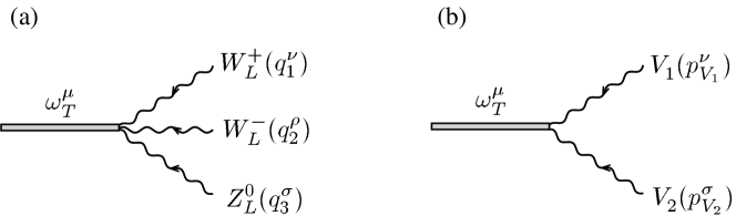
FIG. 1.: Effective interactions of $\omega_{T}$ with (a) $w^{+}w^{-}z$ and (b) two vector bosons.

III Calculation and Results

We consider the two signal processes which proceed via an intermediate $\omega_{T}$:

$$e^{-}\gamma \to e^{-}\omega_{T}\to e^{-}Z\gamma,$$ (12)

$$e^{-}\gamma \to e^{-}\omega_{T}\to e^{-}W^{+}W^{-}Z.$$ (13)

Depending upon the $\omega_{T}Z\gamma$ coupling, the signal cross section can be fairly large. The cross section expressions are lengthy and we do not present them here. We choose to look at these $Z\gamma$ and $WWZ$ final states based on the distinctive signature of the first process and the potential enhancement of the second arising from its dependence on the strong coupling $g_{\omega}$.

The SM background to the process $e\gamma\to eZ\gamma$ is the bremsstrahlung of photons and $Z$’s from the electron. The background process to the $e^{-}W^{+}W^{-}Z$ final state has a complicated structure, with 90 diagrams. The main contribution comes from the subprocesses $e^{+}e^{-}\to W^{+}W^{-},\gamma\gamma\to W^{+}W^{-}$ with a radiated $Z$. We use the MADGRAPH package [8] to evaluate the full SM amplitudes for the background processes.

In calculating the total cross sections for the $eZ\gamma$ signal and the backgrounds, we impose the following “basic cuts” to roughly simulate the detector coverage:

$$170^{\circ}>\theta_{e}>10^{\circ},\quad 165^{\circ}>\theta_{\gamma}>15^{\circ},\quad\theta_{e\gamma}>30^{\circ},\quad E_{\gamma}>50\ {\rm GeV},$$ (14)

where $\theta_{e}$ is the polar angle with respect to the $e^{-}$ beam direction in the lab ($e^{+}e^{-}$ c. m.) frame and $\theta_{e\gamma}$ is the angle between the outgoing $e^{-}$ and $\gamma$. Only the cut on $\theta_{e}$ is relevant to the $e^{-}W^{+}W^{-}Z$ process. The cuts on photons also regularize the infrared and collinear divergences in the tree-level background calculations.

We have also implemented the back-scattered laser spectrum for the photon beam [9]. For simplicity, we have ignored the possible polarization for the electron and photon beams, although an appropriate choice of photon beam polarization may enhance the signal and suppress the backgrounds.

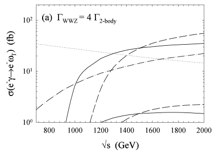
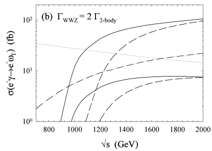
FIG. 2.: Cross sections versus the $e^{+}e^{-}$ c. m. energy for the signal $e^{-}\gamma\to e^{-}\omega_{T}$ with $\omega_{T}\to W^{+}W^{-}Z$ and $Z\gamma$ and the SM backgrounds. The solid lines are for $M_{\omega_{T}}=0.8$ TeV and the long-dashed lines for $M_{\omega_{T}}=1.0$ TeV. In each case the curve with the larger cross section is for the $W^{+}W^{-}Z$ final state and the lower for the $Z\gamma$ final state. The dash-dot line is for the $e^{-}W^{+}W^{-}Z$ SM background and the dotted line is for the $e^{-}Z\gamma$ SM background. In (a), $\Gamma_{WWZ}=4\Gamma_{2-body}$ and in (b), $\Gamma_{WWZ}=2\Gamma_{2-body}$. The chosen values of the partial widths are given in the text.

We present the total cross section for the signal and background versus the $e^{+}e^{-}$ c. m. energy $\sqrt{s_{e^{+}e^{-}}}$ in Fig. 2 with various choices of $\omega_{T}$ mass and partial widths. We have taken representative values for $M_{\omega_{T}}$ of 0.8 (1.0) TeV. In Fig. 2(a), we use partial widths $\Gamma_{2-body}=5$ (20) GeV and $\Gamma_{WWZ}=20$ (80) GeV, setting $\Gamma_{WWZ}=4\Gamma_{2-body}$. In Fig. 2(b), we take $\Gamma_{2-body}=15$ (40) GeV and $\Gamma_{WWZ}=30$ (80) GeV, such that $\Gamma_{WWZ}=2\Gamma_{2-body}$. As noted above, the values for the couplings $\chi$ and $g_{\omega}$ are obtained using these partial widths as input. In Fig. 2(b), the 2-body decay modes represent a larger fraction of the total width and, hence, the cross sections for the signal processes, which go via $Z\gamma$ fusion, are enhanced due to the larger value of $\chi$. We see that, for the parameters considered, the signal cross sections for the $e^{-}W^{+}W^{-}Z$ channel are about $10-100$ fb once above the $\omega_{T}$ mass threshold and overtake the background rates by as much as an order of magnitude. Such high production rates imply that the linear collider would have great potential to discover and study the $\omega_{T}$. The cross sections for the $Z\gamma$ final state are lower, as expected, and lie below the background when only the cuts of Eq. (14) are imposed.

The reason that the cross section for $M_{\omega_{T}}=1.0$ TeV becomes larger than that for 0.8 TeV in Fig. 2(a) is because we have chosen relatively larger couplings for the 1.0 TeV $\omega_{T}$, based on the larger input partial widths.

In Fig. 3, we show the total signal cross sections versus $M_{\omega_{T}}$ for $\sqrt{s_{e^{+}e^{-}}}$=1.5 TeV. The couplings are the values obtained by taking $\Gamma_{2-body}=1\%M_{\omega_{T}}$ and $\Gamma_{WWZ}=4\Gamma_{2-body}$. As expected, below the mass threshold $\sqrt{s_{e\gamma}}<M_{\omega_{T}}$, the signal cross section drops sharply. However, depending on the broadness of the resonance, there is still non-zero signal cross section.

FIG. 3.: Cross sections versus the $M_{\omega_{T}}$ for the signal $e^{-}\gamma\to e^{-}\omega_{T}$ for $\sqrt{s_{e^{+}e^{-}}}=1.5$ TeV with $\omega_{T}\to W^{+}W^{-}Z$ (dashed line) and $Z\gamma$ (solid line).

We have chosen partial decay widths of $\omega_{T}$ as input parameters to characterize its coupling strength. It is informative to explore how the cross section changes with the widths. Fig. 4 demonstrates this point, for $\sqrt{s_{e^{+}e^{-}}}$=1.5 TeV and $M_{\omega_{T}}$=1 TeV. We vary $\Gamma_{2-body}$ and take $\Gamma_{WWZ}=4\Gamma_{2-body}$. Measurement of the signal cross section rates and relative branching fractions for the two channels would reveal important information on the underlying SEWS dynamics.

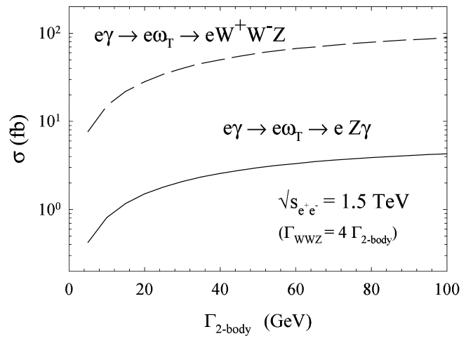
FIG. 4.: Cross sections versus the partial width $\Gamma_{2-body}$ for the signal $e^{-}\gamma\to e^{-}\omega_{T}$ for $\sqrt{s_{e^{+}e^{-}}}=1.5$ TeV and $M_{\omega_{T}}=1$ TeV with $\omega_{T}\to W^{+}W^{-}Z$ (dashed line) and $Z\gamma$ (solid line).

Although the SM backgrounds seem to be larger or, at best comparable, to the signal rate for the $Z\gamma$ channel, the final state kinematics is very different between them. Because the final state vector bosons in the signal are from the decay of a very massive particle, they are generally very energetic and fairly central. We thus impose further cuts to reduce the backgrounds at little cost to the signal:

$$15^{\circ}<\theta_{\gamma,Z,W}<165^{\circ},\quad E_{\gamma,Z,W}>150\ {\rm GeV}.$$ (15)

The most distinctive feature for the signal is the resonance in the invariant mass spectrum for $W^{+}W^{-}Z$ and $Z\gamma$ final states. We demonstrate this in Fig. 5 for both the $W^{+}W^{-}Z$ and $Z\gamma$ modes. Results for $M_{\omega_{T}}$ of 0.8 TeV (dotted lines) and 1.0 TeV (dashed lines) are shown for $\sqrt{s_{e^{+}e^{-}}}=1.5$ TeV. We take $\Gamma_{WWZ}=2\Gamma_{2-body}$. The cuts in both Eqs. (14) and (15) are imposed. We see that a resonant structure at $M_{\omega_{T}}$ is evident and the SM backgrounds (solid lines) after cuts (15) are essentially negligible for the particular choice of parameters shown.

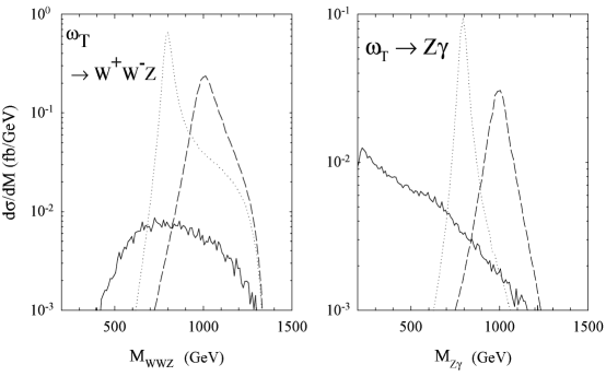
FIG. 5.: Differential cross sections for $\sqrt{s_{e^{+}e^{-}}}=1.5$ TeV as a function of the invariant mass of the $\omega_{T}$ decay products $M(WWZ)$ and $M(Z\gamma)$ for the signal $e^{-}\gamma\to e^{-}\omega_{T}$ with $\omega_{T}\to W^{+}W^{-}Z$ and $Z\gamma$. The dotted lines are for ${M_{\omega_{T}}}=0.8$ TeV and the dashed lines for ${M_{\omega_{T}}}=1.0$ TeV, with $\Gamma_{WWZ}=2\Gamma_{2-body}$ in each case. The SM background relevant to each case are given by the solid lines.

To further assess the discovery potential, we explore the parameter space for $M_{\omega_{T}}$ and $\Gamma_{\omega_{T}}$ at a 1.5 TeV linear collider. The signal for the $WWZ$ mode consists of both $W$’s decaying hadronically and the $Z$ decaying hadronically or into electrons or muons. The same $Z$ decay modes provide the signal for the $Z\gamma$ channel, along with the detected photon. We assume an 80% detection efficiency for each of the $W$, $Z$, and $\gamma$ and an integrated luminosity of 200 fb^-1. In Fig. 6, we give contours representing 3$\sigma$ and 5$\sigma$ discovery limits for the two cases of $\Gamma_{WWZ}=2\Gamma_{2-body}$ (solid lines) and $\Gamma_{WWZ}=4\Gamma_{2-body}$ (dashed lines). For these results, both cuts (14) and (15) are imposed. In addition, a cut about the invariant masses $M_{WWZ},M_{Z\gamma}\pm\Gamma_{\omega_{T}}$ is made for the signals and backgrounds. The two channels are combined by convolution of the product of their respective Gaussian probability functions. We present the results for the techniomega mass and width range at the limit of its resonance production at a 1.5 TeV collider. As an example, from Fig. 6, we see that for $\Gamma_{\omega_{T}}$ of 100 GeV, an $\omega_{T}$ can be detected at the 3$\sigma$ level up to $M_{\omega_{T}}$ of about 1340 GeV for $\Gamma_{WWZ}=4\Gamma_{2-body}$ and up to 1355 GeV for $\Gamma_{WWZ}=2\Gamma_{2-body}$.

FIG. 6.: Contours representing 3$\sigma$ and 5$\sigma$ $\omega_{T}$ discovery limits in the parameter space for $M_{\omega_{T}}$ and $\Gamma_{\omega_{T}}$ with $\sqrt{s_{e^{+}e^{-}}}=1.5$ TeV and an integrated luminosity of 200 fb^-1. Two choices of the ratio of $\Gamma_{WWZ}$ to $\Gamma_{2-body}$ are shown.

IV Conclusions

A high energy $e\gamma$ collider is unique in producing an isosinglet vector state such as $\omega_{T}$. We calculated the signal cross sections for processes (12) and (13) in an effective Lagrangian framework. We found that signal rates can be fairly large once above the $M_{\omega_{T}}$ threshold, although the determining factor is the effective electroweak coupling of the $\omega_{T}$, parametrized by $\chi$. The signal characteristics are very different from the SM backgrounds, making the discovery and further study of $\omega_{T}$ physics very promising at the linear collider. With an integrated luminosity of 200 fb^-1 at $\sqrt{s_{e^{+}e^{-}}}=1.5$ TeV, one may discover an $\omega_{T}$ for a broad range of masses and widths, as indicated in Fig. 6.

REFERENCES

[1] For recent reviews on weakly coupled electroweak
sector, see e.g., H. E. Haber, T. Han, F. Merritt and J. Womersley,
hep-ph/9703391, 1996 DPF/DPB Summer Study on
New Directions for High-Energy Physics
Snowmass, CO, 25 Jun - 12 Jul 1996;
Perspectives on Higgs Physics II,
Gordon L. Kane ed., World Scientific, Singapore (1997).
[2] For recent reviews on strongly coupled electroweak
sector, see e.g.,
R.S. Chivukula, M.J. Dugan, M. Golden, E.H. Simmons,
Ann. Rev. Nucl. Part. Sci. 45 255 (1995);
T. Barklow et al., hep-ph/9704217,
1996 DPF/DPB Summer Study on New Directions for High-Energy Physics
Snowmass, CO, 25 Jun - 12 Jul 1996;
T. Han, hep-ph/9704215,
in Tegernsee 1996, The Higgs puzzle, p.197,
Ringberg, Germany, 8-13 Dec 1996.
[3] For a modern review on technicolor theories,
see i.e. K. Lane, hep-ph/9610463,
published in ICHEP 96: p.367.
[4]
See for example, M. Golden, T. Han, and G. Valencia,
Electroweak Symmetry Breaking and New Physics at the TeV Scale,
ed. T.L. Barklow, S. Dawson, H.E. Haber, and J.L. Siegrist, (World
Scientific, Singapore, 1996) p. 292 [hep-ph/9511206] and references
therein; J. Bagger, V. Barger, K. Cheung, J. Gunion, T. Han, G. Ladinsky,
R. Rosenfeld and C.P. Yuan, Phys. Rev. D49, 1246 (1994);
Phys. Rev. D52, 3878 (1995).
[5]
R.S. Chivukula and M. Golden, Phys. Rev. D41, 2795 (1990).
[6]
J. Rosner and R. Rosenfeld, Phys. Rev. D38, 1530 (1988);
R. Rosenfeld, Phys. Rev. D39, 971 (1989).
[7]
T. Han, Z. Huang and P.Q. Hung, Mod. Phys. Lett. A11, 1131 (1996).
[8] T. Stelzer and W. Long,
Comput. Phys. Commun. 81, 357 (1994).
[9]
I.F. Ginzburg et al., Nucl. Instrum. Methods, 205, 47
(1983); 219, 5 (1984).
C. Akerlof, Ann Arbor report UM HE 81-59 (1981; unpublished).