TTP98-38

October 1998

Photon Fragmentation at LEP

A. Gehrmann–De Ridder Institut für Theoretische Teilchenphysik, Universität Karlsruhe,
D-76128 Karlsruhe, Germany

The production of final state photons in hadronic $Z$-boson decays can be used to study the quark-to-photon fragmentation function $D_{q\to\gamma}(z,\mu_{F})$. Currently, two different observables are used at LEP to probe this function: the ‘photon’ + 1 jet rate and the inclusive photon energy distribution. We outline the results of a calculation of the ‘photon’ + 1 jet rate at fixed ${\cal O}(\alpha\alpha_{s})$, which yield a next-to-leading order determination of the quark-to-photon fragmentation function $D_{q\to\gamma}(z,\mu_{F})$. The resulting predictions for the isolated photon rate and the inclusive photon spectrum at the same, fixed order, are found to be in good agreement with experimental data. Furthermore, we outline the main features of conventional approaches using parameterizations of the resummed solutions of the evolution equation and point out deficiencies of these currently available parameterizations in the large $z$-region. We finally demonstrate that the ALEPH data on the ‘photon’ + 1 jet rate are able to discriminate between different parameterizations of the quark-to-photon fragmentation function, which are equally allowed by the OPAL photon energy distribution data.

1 Introduction

The production of final state photons at large transverse momenta is one of the key observables studied in hadronic collisions. Data on high-$p_{T}$ photon production yield valuable information on the gluon distribution in the proton, while the presence of photons in the final state represents an important background source in many searches for new physics. A good understanding of direct photon production within the context of the Standard model is therefore essential.

Photons produced in hadronic collisions arise essentially from two different sources: the direct production of a photon off a primary parton or through the fragmentation of a hadronic jet into a single photon carrying a large fraction of the jet energy. The former gives rise to perturbatively calculable short-distance contributions whereas the latter is primarily a long distance process which cannot be calculated within perturbative QCD. It is described by the process-independent parton-to-photon fragmentation function [1] which must be determined from experimental data. Its evolution with the factorization scale $\mu_{F}$ can however be determined by perturbative methods.

Directly emitted photons are usually well separated from all hadron jets produced in a particular event, while photons originating from fragmentation processes are primarily to be found inside hadronic jets. Consequently, by imposing some isolation criterion on the photon, one is in principle able to suppress (but not to eliminate) the fragmentation contribution to final state photon cross sections, and thus to define isolated photons. However, recent analyses of the production of isolated photons in electron-positron and proton-antiproton collisions have shown that the application of a geometrical isolation cone surrounding the photon does not lead to a reasonable agreement between theoretical prediction and experimental data.

An alternative approach to study final state photons produced in a hadronic environment is obtained by applying the so-called democratic clustering procedure [2]. In this approach, the photon is treated like any other hadron and is clustered simultaneously with the other hadrons into jets. Consequently, one of the jets in the final state contains a photon and is labelled ‘photon jet’ if the fraction of electromagnetic energy within the jet is sufficiently large,

$$z=\frac{E_{EM}}{E_{EM}+E_{HAD}}>z_{\rm cut},$$ (1)

with $z_{\rm cut}$ determined by the experimental conditions. This photon is called isolated if it carries more than a certain fraction, typically 95%, of the jet energy and said to be non-isolated otherwise. Note that this separation is made by studying the experimental $z$ distribution and is usually such that hadronisation effects, which tend to reduce $z$, are minimized.

This democratic procedure has been applied by the ALEPH collaboration at CERN in an analysis of two jet events in electron-positron annihilation in which one of the jets contains a highly energetic photon [3]. In this analysis, ALEPH made a leading order determination of the quark-to-photon fragmentation function by comparing the photon + 1 jet rate calculated up to ${\cal O}(\alpha)$ [2] with the data. The theoretical basis on which the measurement of the ‘photon’ + 1 jet rate relies, is an explicit counting of powers of the strong coupling $\alpha_{s}$ in both the direct and the fragmentation contributions, no resummation of $\ln\mu_{F}^{2}$ is performed. We shall refer to this theoretical framework as the fixed order approach. In Section 2, we will describe the main features of the leading and next-to-leading order calculation of the photon + 1 jet rate following this fixed order approach and see how the obtained predictions compare with the available data.

More recently, the OPAL collaboration has measured the inclusive photon distribution for final state photons with energies as small as 10 GeV [4]. This corresponds to the photon carrying a fraction of the beam momentum, $x_{\gamma}$, to be as low as 0.2. They have compared their results with the two model-dependent predictions of GRV [5] and BFG [6] and found a reasonable agreement in both cases when choosing the factorization scale $\mu_{F}=M_{Z}$. In Section 2 we shall compare the predictions obtained for the inclusive rate within our fixed order approach with the OPAL data too.

The model predictions [5, 6] mentioned above are based on a resummation of the logarithms of the factorization scale $\mu_{F}$ and naturally associate an inverse power of $\alpha_{s}$ with all fragmentation contributions. We shall refer to this resummation procedure as the conventional approach. In Section 3 we shall present the main features of this approach, outline the results obtained for the photon + 1 jet rate in this approach while using either the GRV or BFG parameterizations for the photon fragmentation function and show how these compare with the ALEPH data. Finally Section 4 contains our conclusions.

2 The photon + 1 jet rate in the fixed order framework

2.1 The photon + 1 jet rate at ${\cal O}(\alpha)$

In the fixed order framework, the cross section for the production of isolated photons receives sizeable contributions from both direct photon and fragmentation processes. More precisely, the distribution of electromagnetic energy within the photon jet of photon + 1 jet events, for a single quark of charge $e_{q}$, at ${\cal O}(\alpha)$ in the $\overline{{\rm MS}}$-scheme, can be written as [2],

$$\frac{1}{\sigma_{0}}\frac{{\rm d}\sigma^{(LO)}}{dz} = 2D_{q\to\gamma}(z,\mu_{F})+\frac{\alpha e_{q}^{2}}{\pi}P_{q\gamma}^{(0)}(z)\log\left(\frac{s_{\rm cut}}{\mu_{F}^{2}}\right)\,+\,R_{\Delta}\delta(1-z)+\ldots,$$ (2)

$$= 2D_{q\to\gamma}(z,\mu_{F})+C_{\gamma}^{(0)}(z,\mu_{F}).$$

The $\ldots$ represent terms which are well behaved as $z\to 1$. $C^{(0)}_{\gamma}$ is the coefficient function corresponding to the lowest order process $e^{+}e^{-}\to q\bar{q}\gamma$. It is defined after the leading quark-photon singularity has been subtracted and factorized in the bare quark-to-photon fragmentation function in the $\overline{{\rm MS}}$ scheme. The non-perturbative fragmentation function is an exact solution at ${\cal O}(\alpha)$ of the evolution equation in the factorization scale $\mu_{F}$,

$$D_{q\to\gamma}(z,\mu_{F})=\frac{\alpha e_{q}^{2}}{2\pi}P_{q\gamma}^{(0)}(z)\log\left(\frac{\mu_{F}^{2}}{\mu_{0}^{2}}\right)+D_{q\to\gamma}(z,\mu_{0}).$$ (3)

In this equation, all unknown long-distance effects are related to the behaviour of $D_{q\to\gamma}(z,\mu_{0})$, the initial value of this fragmentation function which has been fitted to the data at some initial scale $\mu_{0}$ in [3]. As $D_{q\to\gamma}(z,\mu_{F})$ is exact, this solution does not take the commonly implemented [5, 6] resummations of $\log(\mu_{F}^{2})$ into account and when used to evaluate the photon + 1 jet rate at ${\cal O}(\alpha)$ yields a factorization scale independent prediction for the cross section.

In the Durham jet algorithm, $s_{\rm cut}\sim sz(1-z)^{2}/(1+z)\sim p_{T}^{2}$ [7] where $p_{T}$ is the transverse momentum of the photon with respect to the cluster. For $z<1$, we find that $\mu_{F}^{2}\sim s_{\rm cut}$ and $\mu_{F}^{2}\gg\mu_{0}^{2}$ . The ‘direct’ contribution in eq. (2) is therefore suppressed relative to the fragmentation contribution. The conventional assignment of a power of $1/\alpha_{s}$ to the fragmentation function can in this case be motivated, this contribution is indeed more significant. However, as $z\to 1$, we see that the transverse size of the photon jet cluster decreases such that $s_{\rm cut}\to 0$. The hierarchy $s_{\rm cut}\sim\mu_{F}^{2}$ and $\mu_{F}^{2}\gg\mu_{0}^{2}$ is no longer preserved and both contributions in eq. (2) are important. Large logarithms of $(1-z)$ become the most dominant contributions. Being primarily interested in the high $z$ region, in [2] it was chosen not to impose the conventional prejudice and resum the logarithms of $\mu_{F}$ a priori but to work within a fixed order framework, to isolate the relevant large logarithms.

We have performed the calculation of the ${\cal O}(\alpha_{s})$ corrections to the ‘photon’ + 1 jet rate using the same democratic procedure to define the photon as in [2, 3]. The details of this fixed order calculation have been presented in  [8]. In the following, we shall limit ourselves to outline the main characteristics of this calculation, to summarize the results and to show how these compare with the available experimental data from ALEPH.

2.2 The ‘photon’ + 1 jet rate at ${\cal O}(\alpha\alpha_{s})$

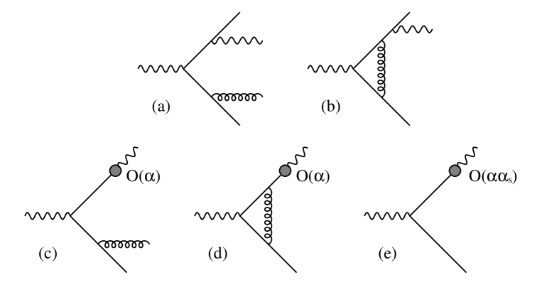
Figure 1: Parton level subprocesses contributing to the photon + 1 jet rate at ${\cal O}(\alpha\alpha_{s})$.

The ‘photon’ + 1 jet rate in $e^{+}e^{-}$ annihilation at ${\cal O}(\alpha\alpha_{s})$ receives contributions from five parton-level subprocesses displayed in Fig. 1. Although the ‘photon’ + 1 jet cross section is finite at ${\cal O}(\alpha\alpha_{s})$, all these contributions contain divergences (when the photon and/or the gluon are collinear with one of the quarks, when the gluon is soft or since the bare quark-to-photon fragmentation function contains infinite counter terms). All these divergences have to be isolated and cancelled analytically before the ‘photon’ + 1 jet cross section can be evaluated numerically.

The various configurations where the tree level process $\gamma^{*}\to q\bar{q}g\gamma$ contributes to the photon + 1 jet rate are illustrated in Fig. 2.

Figure 2: Different final state ‘photon’ + 1 jet topologies arising from the tree level $\gamma^{*}\to q\bar{q}\gamma g$ process. The ‘photon’ jet is moving to the left while the recoiling hadronic jet moves to the right. Square brackets denote theoretically unresolved particles, round brackets experimental clusters.

The associated real contributions can be separated into three categories: either theoretically resolved, single unresolved or double unresolved. Within each singular region which is defined using a theoretical criterion $s_{\rm min}$, the matrix elements are approximated and the unresolved variables analytically integrated. The evaluation of the singular contributions associated with the process $\gamma^{*}\to q\bar{q}g\gamma$ is of particular interest as it contains various ingredients which could directly be applied to the calculation of jet observables at next-to-next-to-leading order. Indeed, besides the contributions arising when one final state gluon is collinear or soft (single unresolved contributions, see fig.2(b)), there are also contributions where two of the final state partons are theoretically unresolved, see fig.2(c) . The three different double unresolved contributions which occur in this calculation are: the triple collinear contributions, arising when the photon and the gluon are simultaneously collinear to one of the quarks, the soft/collinear contributions arising when the photon is collinear to one of the quarks while the gluon is soft and the double single collinear contributions, resulting when the photon is collinear to one of the quarks while the gluon is collinear to the other. A detailed derivation of each of these singular real contributions and of the singular contributions arising in the processes depicted in Fig. 1(b)-(d) has been presented in [8].

Combining all unresolved contributions present in the processes shown in Fig. 1(a)-(d) yields a result that still contains single and double poles in $\epsilon$. These pole terms are however proportional to the universal next-to-leading order splitting function $P_{q\gamma}^{(1)}$  [9] and a convolution of two lowest order splitting functions, $(P_{qq}^{(0)}\otimes P_{q\gamma}^{(0)})$. Hence, they can be factorized into the next-to-leading order counterterm of the bare quark-to photon fragmentation function [10] present in the contribution depicted in Fig. 1(e), yielding a finite and factorization scale ($\mu_{F}$) dependent result [8].

We have then chosen to evaluate the remaining finite contributions numerically using the hybrid subtraction method, a generalization of the phase space slicing procedure [11, 12]. The latter procedure turns out to be inappropriate when more than one particle is potentially unresolved. Indeed, in our calculation we found areas in the four parton phase space which belong simultaneously to two different single collinear regions. Those areas cannot be treated correctly within the phase space slicing procedure. Within the hybrid subtraction method developed in [13], a parton resolution criterion $s_{\rm min}$ is used to separate the phase space into different resolved and unresolved regions. Phase space slicing and hybrid subtraction methods vary only in the numerical treatment of the unresolved regions. While the matrix elements are set to zero in the former method, one considers the difference between the full matrix element and its approximation in all unresolved regions in the latter. The non-singular contributions are calculated using Monte Carlo methods like in the phase space slicing scheme.

The numerical program finally evaluating the ‘photon’ + 1 jet rate at ${\cal O}(\alpha\alpha_{s})$ contains four separate contributions.

Figure 3: ${\cal O}(\alpha\alpha_{s})$ individual contributions (left) and sum of all ${\cal O}(\alpha\alpha_{s})$ contributions (right) to the photon + 1 jet rate for a single quark of charge $e_{q}$ such that $\alpha e_{q}^{2}=2\pi$, $\alpha_{s}(N^{2}-1)/2N=2\pi$ using the Durham jet algorithm with $y_{{\rm cut}}=0.1$, and integrated for $z>0.7$.

Each of them depends logarithmically (in fact as $\log^{3}(y_{{\rm min}})$) on the theoretical resolution parameter $y_{{\rm min}}=s_{{\rm min}}/Q^{2}$. The physical ‘photon’ + 1 jet cross section, which is the sum of all four contributions, must of course be independent of the choice of $y_{{\rm min}}$, the latter being just an artefact of the theoretical calculation. In Fig. 3, we see that the cross section approaches (within numerical errors) a constant value provided that $y_{{\rm min}}$ is chosen small enough, indicating that a complete cancellation of all powers of $\log(y_{{\rm min}})$ takes place. This provides a strong check on the correctness of our results and on the consistency of our approach.

Finally, after factorization of the quark-photon singularities, the ${\cal O}(\alpha\alpha_{s})$ cross section takes the following form,

$$\frac{1}{\sigma_{0}}\frac{{\rm d}\sigma^{(NLO)}}{{\rm d}z}=\frac{1}{\sigma_{0}}\frac{{\rm d}\sigma^{(LO)}}{{\rm d}z}+\left(\frac{\alpha_{s}}{2\pi}\right)\left(\frac{\alpha e_{q}^{2}}{2\pi}\right)C^{(1)}_{\gamma}(z,\mu_{F})+C_{q}^{(0)}\otimes D_{q\to\gamma}(z,\mu_{F}).$$ (4)

The lowest order cross section has been given in eq.(2) while the hard scattering coefficient functions $C_{i}^{(n)}$ appearing explicitly in this equation are defined as follows. The (finite) next-to-leading order coefficient function $C^{(1)}_{\gamma}$ is obtained numerically after the next-to-leading quark-photon singularity has been subtracted. More precisely, $C^{(1)}_{\gamma}$ is obtained after summing all contributions which are independent of $D_{q\to\gamma}(z,\mu_{F})$ arising from the Feynman diagrams depicted in Fig. 1 together. A detailed description of the evaluation of $C^{(1)}_{\gamma}$ has been given in [8]. The coefficient function $C_{q}^{(0)}$ is the finite part associated with the sum of real and virtual gluon contributions to the process $e^{+}e^{-}\to q\bar{q}$. It is straightforward to evaluate, and can be found for example in [14].

2.3 Comparison with Experimental Data

A comparison between the measured ‘photon’ + 1 jet rate [3] and our calculation yielded a first determination of the quark-to-photon fragmentation function accurate up to ${\cal O}(\alpha\alpha_{s})$ [15]. This function, which parameterizes the perturbatively incalculable long-distance effects, has to satisfy a perturbative evolution equation in the factorization scale $\mu_{F}$. At next-to-leading order (${\cal O}(\alpha\alpha_{s})$) this equation reads,

$$\frac{\partial D_{q\to\gamma}(z,\mu_{F})}{\partial\log(\mu_{F}^{2})}=\left(\frac{\alpha e_{q}^{2}}{2\pi}\right)P^{(0)}_{q\to\gamma}(z)\,+\,\left(\frac{\alpha e_{q}^{2}}{2\pi}\right)\left(\frac{\alpha_{s}}{2\pi}\right)P^{(1)}_{q\to\gamma}(z)+\left(\frac{\alpha_{s}}{2\pi}\right)P^{(0)}_{q\to q}\otimes D_{q\to\gamma}(z,\mu_{F}).$$ (5)

$P^{(0)}_{q\to q}$ and $P^{(1)}_{q\to\gamma}$ are respectively the lowest order quark-to-quark and the next-to-leading order quark-to-photon universal splitting functions [9, 16, 17]. The next-to-leading order fragmentation function can be expressed as an exact solution of this evolution equation up to ${\cal O}(\alpha\alpha_{s})$ [8],

$$D_{q\to\gamma}(z,\mu_{F}) = \frac{\alpha e_{q}^{2}}{2\pi}P^{(0)}_{q\gamma}(z)\log\left(\frac{\mu^{2}_{F}}{\mu_{0}^{2}}\right)+\frac{\alpha e_{q}^{2}}{2\pi}\frac{\alpha_{s}}{2\pi}\left(\frac{N^{2}-1}{2N}\right)P_{q\gamma}^{(1)}(z)\log\left(\frac{\mu^{2}_{F}}{\mu_{0}^{2}}\right)$$ (6)

$$+\frac{\alpha_{s}}{2\pi}\left(\frac{N^{2}-1}{2N}\right)\log\left(\frac{\mu^{2}_{F}}{\mu_{0}^{2}}\right)P_{qq}^{(0)}(z)\otimes\frac{\alpha e_{q}^{2}}{2\pi}\frac{1}{2}P_{q\gamma}^{(0)}(z)\log\left(\frac{\mu^{2}_{F}}{\mu_{0}^{2}}\right)$$

$$+\frac{\alpha_{s}}{2\pi}\left(\frac{N^{2}-1}{2N}\right)\log\left(\frac{\mu^{2}_{F}}{\mu_{0}^{2}}\right)P_{qq}^{(0)}(z)\otimes D(z,\mu_{0})\,+D(z,\mu_{0}).$$

The initial function $D_{q\to\gamma}^{(NLO)}(z,\mu_{0})$ has been fitted to the ALEPH  1 jet data [15] for $\frac{1}{\sigma_{0}}\frac{d\sigma}{dz}$, for the jet resolution parameter $y_{{\rm cut}}=0.06$ and $\alpha_{s}(M_{z}^{2})=0.124$ to yield ,

$$D^{(NLO)}(z,\mu_{0})=\frac{\alpha e_{q}^{2}}{2\pi}\left(-P^{(0)}_{q\gamma}(z)\log(1-z)^{2}\;+\,20.8\,(1-z)-11.07\right),$$ (7)

where $\mu_{0}=0.64$ GeV. The next-to-leading order ($\overline{{\rm MS}}$) quark-to-photon fragmentation function (for a quark of unit charge) at a factorization scale $\mu_{F}=M_{Z}$ were shown in [15] and compared with the lowest order fragmentation function obtained in [3]. A large difference between the leading and next-to-leading order quark-to-photon fragmentation functions was observed only for $z$ close to 1, indicating the presence of large $\log(1-z)$ terms.

Moreover, a comparison between the ALEPH data and the results of the ${\cal O}(\alpha\alpha_{s})$ calculation using the fitted next-to-leading order fragmentation function for different values of $y_{\rm cut}$ can be found in [8, 15]. The next-to-leading order corrections were found to be moderate for all values of $y_{\rm cut}$ demonstrating the perturbative stability of our fixed order approach.

Figure 4: The integrated photon + 1 jet rate above $z=0.95$ as function of $y_{{\rm cut}}$, compared with the ${\cal O}(\alpha)$ and ${\cal O}(\alpha\alpha_{s})$ order calculations including the appropriate quark-to-photon fragmentation functions.

To test the generality of our results, we have considered two further applications: the ‘isolated’ photon rate and the inclusive photon distribution which we shall now briefly present.

Using the results of the calculation of the photon + 1 jet rate at ${\cal O}(\alpha\alpha_{s})$ and the fitted quark-to-photon fragmentation function, we have determined the isolated rate defined as the photon + 1 jet rate for $z>0.95$ in the democratic approach. The result of this calculation compared with data from ALEPH [3] and the leading order calculation [2] is shown in Fig. 4. It can clearly be seen that inclusion of the next-to-leading order corrections improves the agreement between data and theory over the whole range of $y_{{\rm cut}}$. It is also apparent that the next-to-leading order corrections to the isolated photon + 1 jet rate obtained in this democratic clustering approach are of reasonable size indicating a good perturbative stability of this isolated photon definition.

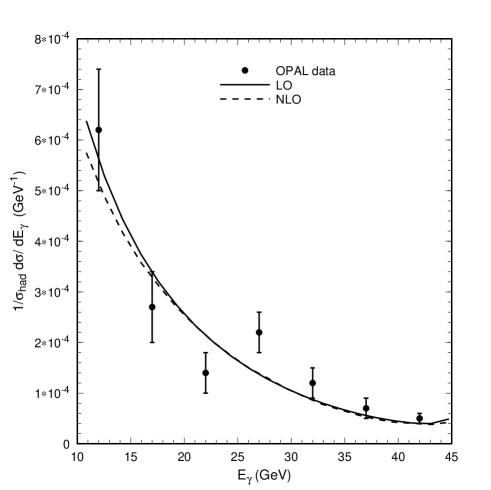
Figure 5: The inclusive photon energy distribution normalized to the hadronic cross section as measured by the OPAL Collaboration compared with the ${\cal O}(\alpha)$ and ${\cal O}(\alpha\alpha_{s})$ order calculations including the appropriate quark-to-photon fragmentation functions determined using the ALEPH photon + 1 jet data.

The OPAL collaboration has recently measured the inclusive photon distribution for final state photons with energies between 10 and 42 GeV [4]. Fig. 5 shows our (scale independent) predictions for the inclusive photon energy distribution at both leading and next-to-leading order. We see good agreement with the data, even though the phase space relevant for the OPAL data, which corresponds to $x_{\gamma}$ values as small as 0.2, far exceeds that used to determine the fragmentation functions from the ALEPH photon + 1 jet data.

3 The photon + 1 jet rate in the conventional approach

In the conventional approach, the parton-to-photon fragmentation function $D_{i\to\gamma}$ satisfies an all order inhomogeneous evolution equation [17]. Usually, these equations can be diagonalized in terms of the singlet and non-singlet quark fragmentation functions as well as the gluon fragmentation function. However when analyzing the global features of the solutions of these evolution equations, as was discussed in [18], several simplifications can be consistently made. For example, the gluon-to-photon fragmentation function is by orders of magnitude smaller than the quark-to-photon fragmentation functions, as was shown in [18]. Its contribution to the photon cross section can safely be ignored. Consequently, the flavour singlet and non-singlet quark-to-photon fragmentation functions become equal to a unique fragmentation function $D_{q\to\gamma}$ which satisfies an evolution equation having a similar form than the next-to-leading order evolution valid in the fixed order approach, see eq. (5). Unlike in eq. (5) though, the strong coupling $\alpha_{s}$ is now a function of the factorization scale, it runs.

The full solution $D_{q\to\gamma}$ of the inhomogeneous evolution equation is given by the sum of two contributions; a pointlike (or perturbative) part $D_{q\to\gamma}^{pl}$ which is a solution of the inhomogeneous equation follows eq.(5) and a hadronic (or non-perturbative) part $D_{q\to\gamma}^{had}$ which is the solution of the corresponding homogeneous equation. In the conventional approach, approximate solutions of these evolution equations are commonly obtained as follows [5, 6]. First an analytic solution in moment space is obtained in the leading logarithm (LL) or beyond leading logarithm (BLL) approximations. These are then inverted numerically to give the fragmentation function in $x$-space. At LL only terms of the form $(\alpha_{s}^{n}\ln^{n+1}\mu_{F}^{2})$ are kept while at BLL both leading $(\alpha_{s}^{n}\ln^{n+1}\mu_{F}^{2})$ and subleading $(\alpha_{s}^{n}\ln^{n}\mu_{F}^{2})$ logarithms of the mass factorization scale $\mu_{F}$ are resummed to all orders in the strong coupling $\alpha_{s}$.

It is worth noting that both LL and BLL solutions have an asymptotic behaviour given by,

$$D_{q\to\gamma}^{asympt}(z,\mu_{F})=\left(\frac{\alpha e_{q}^{2}}{2\pi}\right)\frac{2\pi}{\alpha_{s}(\mu_{F}^{2})}\,a(z),$$ (8)

where $a(z)$ contains the splitting function $P^{(0)}_{q\to\gamma}$. This asymptotic form lends support to the common assumption that the quark-to-photon fragmentation function $D_{q\to\gamma}$ is ${\cal O}\left(\alpha/\alpha_{s}\right)$. This assumption is in contrast with that adopted in the fixed order approach (cf. Section 2) where the quark-to-photon fragmentation function is ${\cal O}(\alpha)$. It leads to significant differences in the respective expressions of the one-photon production cross sections. Indeed, the LL and BLL expression of the cross section in the $\overline{{\rm MS}}$ scheme arising when one uses the corresponding resummed LL or BLL fragmentation functions in this approach reads

$$\frac{1}{\sigma_{0}}\frac{{\rm d}\sigma^{LL}}{{\rm d}z} = \;D_{q\to\gamma}(z,\mu_{F}),$$

$$\frac{1}{\sigma_{0}}\frac{{\rm d}\sigma^{BLL}}{{\rm d}z} = D_{q\to\gamma}(z,\mu_{F})\,+\left(\frac{\alpha_{s}}{2\pi}\right)C_{q}^{(0)}\otimes D_{q\to\gamma}(z,\mu_{F})+\left(\frac{\alpha e_{q}^{2}}{2\pi}\right)C^{(0)}_{\gamma}(z,\mu_{F}).$$ (9)

As can be seen from these equations, no direct term contributes to the cross section at the LL level, while only the ${\cal O}(\alpha)$ direct term $C^{(0)}_{\gamma}$ contributes at the BLL level to it. At the BLL level, contributions arising from 1(a)-(b) do not enter in the cross section. As explained at length in [15], this conventional procedure of associating an inverse power of $\alpha_{s}$ with the fragmentation function is clearly appropriate when the logarithms of the factorization scale $\mu_{F}$ are the only potentially large logarithms but is problematic when different classes of large logarithms can occur as it is the case in the ‘photon’ + 1 jet cross section.

All unknown long-distance effects are related to the behaviour of the input fragmentation function $D_{q\to\gamma}^{np}(z,\mu_{0})$ implicitly present in eq.(9). In the approaches of GRV or BFG, the non perturbative input function $D_{q\to\gamma}^{np}(z,\mu_{0})$ is treated with only minor differences. Those have been detailed in [18]. We shall here concentrate on the major common points in these approaches. At LL both GRV and BFG agree that $D_{q\to\gamma}^{np}(z,\mu_{0})$ is negligible and can be described by a vector meson dominance model (VMD) as explained in [5] and [6] respectively. However at BLL and in the $\overline{{\rm MS}}$ scheme, the input fragmentation function cannot be negligible due to the presence of the direct term $C_{\gamma}^{(0)}$ and cannot be described by a VMD input alone. Indeed, $C_{\gamma}^{(0)}(z)$ diverges as $z\to 1$ and would drive the cross section to unacceptable negative values if a VMD input alone is considered for the input fragmentation function. Note that the requirement that the cross section is positive led the authors in [2, 15] to consider in the fixed order approach a term proportional to $P^{(0)}_{q\to\gamma}\ln(1-z)^{2}$ in the expression of $D_{q\to\gamma}^{np}(z,\mu_{0})$. In summary, in any resummed or fixed order approach, as soon as the direct term $C_{\gamma}^{(0)}$ enters the cross section, as it does in the $\overline{{\rm MS}}$ factorization scheme, the input fragmentation function $D_{q\to\gamma}^{np}(z,\mu_{0})$ must compensate the large $z$ behaviour of $C_{\gamma}^{(0)}$. Consequently, this input fragmentation function $D_{q\to\gamma}^{np}(z,\mu_{0})$ as well as the total solution $D_{q\to\gamma}(z,\mu_{F})$ in this $\overline{{\rm MS}}$ scheme should clearly exhibit a divergent behaviour as $z\to 1$ .

In Fig. 6 we compare the analytic expression of the fragmentation function obtained in the fixed order approach, eq.(6) with the BLL parameterizations of GRV and BFG for the numerically resummed solutions. We clearly see, that the fixed order solution does diverge as $z\to 1$ while the numerical solutions do not. This significant disagreement is mainly due to deficiencies in the numerical parameterizations. In fact, it can be traced back to the presence of logarithms of $(1-z)$ that are explicit in the expanded result. These logarithms should also be present in the numerical resummed results. However, the parameterizations are necessarily obtained by inverting only a finite number of moments and it is a well known problem to describe a logarithmic behaviour with a polynomial expansion. This clearly indicates that the presently available parameterizations for the resummed fragmentation functions are not accurate at large $z$ and particularly for $z>0.95$.

Figure 6: The quark-to-photon fragmentation function $zD_{u\to\gamma}(z,\mu_{F})$ evaluated at $\mu_{F}=M_{Z}$ in the $(\overline{{\rm MS}})$-scheme. The NLO fit from the ALEPH ‘photon’ + 1 jet data is shown as solid line. The GRV (BFG) parameterization is shown dashed (dotted).

Except in the very high $z$ region however, we see that, the various fragmentation functions generally agree well with each other in shape and magnitude. Consequently we can expect, that predictions for the inclusive photon cross sections (which run over a wide range of $z$) will be largely in agreement, while significant differences may be apparent in the ‘photon’ + 1 jet estimates which focus on the large $z$ region. Indeed, we mentioned that the OPAL data were in agreement with predictions using either (GRV or BFG) parameterizations in the conventional approach, and we showed in Section 2 that these data were also in agreement with the predictions obtained in our fixed order approach.

Let us now concentrate on the ‘photon’ + 1 jet cross section, an observable which is sensitive on the large $z$ region ($0.7<z<1$) and see how the predictions obtained in a conventional approach compare with the ALEPH data. In the following, we focus on one particular value of the jet clustering parameter $y_{\rm cut}$, $y_{\rm cut}=0.1$.

Figure 7: The ‘photon’ + 1 jet rate in the conventional approach using the GRV or the BFG inputs. The experimental data is taken from [3].

Fig. 7 shows the BLL ‘photon’ + 1 jet rates obtained using either the GRV or BFG parameterizations of the photon fragmentation function for $\mu_{F}=M_{Z}$. Ignoring the large $z$ region where we have reason to doubt the accuracy, we see that the BFG predictions lie systematically below that obtained using the GRV parameterization and go through the experimental data points. As discussed in [18], this difference is due to both the choice of hadronic scale and the non-VMD input. The BFG input is smaller and the ‘photon’ + 1 jet data clearly selects this choice. Notice however, that the BFG parameterization for the fragmentation function unlike that of the GRV group was proposed well after the ALEPH data were released.

4 Conclusions

In summary, in Section 2 we have outlined the main features of the calculation [8] of the ‘photon’ + 1 jet rate at ${\cal O}(\alpha\alpha_{s})$. Although only next-to-leading order in perturbation theory, this calculation contains several ingredients appropriate to the calculation of jet observables at next-to-next-to-leading order. In particular, it requires to generalize the phase space slicing method of [11, 12] to take into account contributions where more than one theoretically unresolved particle is present in the final state. The ‘photon’ + 1 jet rate has then been evaluated for a democratic clustering algorithm with a Monte Carlo program using the hybrid subtraction method of [13]. The results of our calculation, when compared to the data [3] on the ‘photon’ + 1 jet rate obtained by ALEPH, enabled a first determination of the process independent quark-to-photon fragmentation function at ${\cal O}(\alpha\alpha_{s})$ in a fixed order approach. As a first application, we have used this function to calculate the ‘isolated’ photon + 1 jet rate in a democratic clustering approach at next-to-leading order. The inclusion of the QCD corrections improves the agreement between theoretical prediction and experimental data. Moreover, it was shown that these corrections are moderate, demonstrating the perturbative stability of this particular isolated photon definition. We have also shown that the inclusive photon energy distribution computed in this fixed order approach and using the quark-to-photon fragmentation function determined with the ALEPH data and is in good agreement with the recent OPAL data.

In Section 3 we have outlined the main characteristics of the conventional approach have described how the LL and BLL solutions of the evolution equation are obtained. An important feature characterizing this approach concerns the power of $\alpha_{s}$ associated to the photon fragmentation function. Although this appears to be ${\cal O}(\alpha)$, inspection of the evolution equation suggests a logarithmic growth with $\mu_{F}$, and in conventional approaches, it is ascribed a nominal power of $\alpha/\alpha_{s}$. Consequences for the LL and BLL cross sections were also discussed in this section.

The full $\mu_{F}$-dependent solution $D_{q\to\gamma}(z,\mu_{F})$ of the evolution can only be obtained provided some non-perturbative input is given. In the approaches of GRV or BFG, this input has two pieces, a small vector meson dominance contribution together with a perturbative counterterm. In either case, we have found that the large $z$ behaviour of the fragmentation functions is not well reproduced by the parameterizations, the main problem being to describe a logarithmic behaviour with a polynomial. Predictions using any of the presently available (GRV or BFG) resummed fragmentation functions do therefore not yield accurate results in the region $z>0.95$. Ignoring this high $z$ region, the BLL predictions for the photon + 1 jet rate obtained using the BFG parameterization are found to be in agreement with the ALEPH data, while the predictions using the fragmentation function of GRV lie too high.

To summarize, we have seen that the inclusive and ‘photon’ + 1 jet data from LEP can be described using either the ${\cal O}(\alpha\alpha_{s})$ fragmentation function whose non-perturbative input is fitted to the ALEPH data or using the BLL parameterization of BFG. In the latter case, the agreement needs however to be restricted to $z$-values below 0.95.

References

-
[1]
K. Koller, T.F. Walsh and P.M. Zerwas, Z. Phys. C2 (1979) 197;
E. Laermann, T.F. Walsh, I. Schmitt and P.M. Zerwas, Nucl. Phys. B207 (1982) 205. - [2] E.W.N. Glover and A.G. Morgan, Z. Phys. C62 (1994) 311.
- [3] ALEPH collaboration: D. Buskulic et al., Z. Phys. C69 (1996) 365.
- [4] OPAL Collaboration: K. Ackerstaff et al., Eur. Phys. J. C2 (1998) 39.
- [5] M. Glück, E. Reya and A. Vogt, Phys. Rev. D48 (1993) 116.
- [6] L. Bourhis, M. Fontannaz and J.Ph. Guillet, Eur. Phys. J. C2 (1998) 529.
- [7] Yu.L. Dokshitzer, Contribution to the Workshop on Jets at LEP and HERA, J. Phys. G17 (1991) 1441.
- [8] A. Gehrmann–De Ridder and E.W.N. Glover, Nucl. Phys. B517 (1998) 269.
-
[9]
G. Curci, W. Furmanski and R. Petronzio, Nucl. Phys. B175 (1980) 27;
W. Furmanski and R. Petronzio, Phys. Lett. 97B (1980) 437. -
[10]
G. Altarelli, R.K. Ellis, G. Martinelli and S.-Y. Pi, Nucl. Phys. B160
(1979) 301;
P.J. Rijken and W.L. van Neerven, Nucl. Phys. B487 (1997) 233. - [11] W.T. Giele and E.W.N. Glover, Phys. Rev. D46 (1992) 1980.
- [12] K. Fabricius, I. Schmitt, G. Kramer and G. Schierholz, Z. Phys. C11 (1981) 315.
- [13] E.W.N. Glover and M.R. Sutton, Phys. Lett. B342 (1995) 375.
- [14] Z. Kunszt and Z. Trócsányi, Nucl. Phys. B394 (1993)139.
- [15] A. Gehrmann–De Ridder, T. Gehrmann and E.W.N. Glover, Phys. Lett. B414 (1997) 354.
- [16] P.J. Rijken and W.L. van Neerven, Nucl. Phys. B487 (1997) 233.
- [17] G. Altarelli and G. Parisi, Nucl. Phys. B126 (1977) 298.
- [18] A. Gehrmann–De Ridder and E.W.N. Glover, preprint DESY-98-068, DTP/98/26 (hep-ph/9806316).