On the Interaction of Monopoles and Domain Walls

Abstract

We study the interaction between monopoles and embedded domain walls in a $O(3)$ linear sigma model. We discover that there is an attractive force between the monopole and the wall. We provide evidence that after the monopole and domain wall collide, the monopole unwinds on the wall, and that the winding number spreads out on the surface. These results support the suggestion by Dvali et al. (hep-ph/9710301) that the monopole problem can be solved by monopole-domain wall interactions.

I Introduction

Monopoles are predicted in all grand unified field theories which are spontaneously broken to yield the Standard Model of strong, weak and electromagnetic interactions [1, 2]. More generally, monopoles arise whenever a symmetry group $G$ is broken to a subgroup $H$ such that the vacuum manifold ${\cal M}$ (which in the case of a simply connected group $G$ is ${\cal M}=G/H$) has nontrivial second homotopy group, i.e. $\Pi_{2}({\cal M})\neq 1$). Zel’dovich and collaborators [3] and Preskill [4] realized that there is a serious conflict between grand unified field theories (GUTs) and standard cosmology: GUT symmetry breaking in the early Universe would produce an over-abundance of monopoles which would overclose the Universe by many orders of magnitude.

The most popular solution of the monopole problem is to invoke a period of inflation [5] after GUT symmetry breaking. Inflation will exponentially dilute the number density of monopoles. Since inflation is likely generated by a sector of the theory that is only weakly coupled to standard model fields, it is quite possible that the GUT symmetry is not broken after inflation, and hence that the monopole problem re-emerges. Within the context of explosive energy transfer during inflationary reheating [6] (“preheating” [7]) it is also possible that monopoles may be generated during reheating [8, 9, 10, 11].

There are other possible solutions of the monopole problem, e.g. the Langacker-Pi mechanism [12] in which the symmetry is partially restored at some intermediate time (which leads to the decay of the heavy monopoles), or the anti-unification scenario [13, 14] in which the GUT symmetry is never restored. These mechanisms, however, require a substantial amount of particle physics fine tuning.

Recently, Dvali et al. [15] have proposed a new solution to the monopole problem. They consider a theory in which, in addition to monopoles, domain walls are also present. It was conjecttured that the domain walls would sweep up monopoles and antimonopoles and, if a local attractive force between monopole and domain wall exists, the monopole charge would diffuse onto the domain wall. This would then lead to an annihilation between monopole and antimonopole charge, thus solving the monopole problem.

To provide evidence in support of the Dvali et al. mechanism it is crucial to study the following issues:

1. Is there an attractive force between a monopole and a domain wall?

2. If 1 is correct, then is there scattering, transmission or does the monopole unwind upon contact with the domain wall?

We study these issues using a scalar field theory with an internal symmetry of $O(3)$ breaking spontaneously to $SO(2)$. This theory admits both embedded domain walls and global monopoles. The monopoles are topologically stable, whereas the embedded walls are not stable [16]. However, we find that the embedded walls in our simulation have a sufficiently long decay time so that the interaction between a monopole and the wall can be studied.

Based on our numerical study, we find that there is an attractive force between the monopole and the wall. Furthermore, we provide evidence that, upon contact, the monopole unwinds on the wall, with the winding number spreading out on the surface.

Ideally, one would like to study the interaction of local monopoles and topologically stable domain walls. For computational reasons we have decided to begin with an analysis of global monopoles interacting with embedded walls, a problem involving many fewer fields. We are interested in local forces rather than global confiugurations, and we give qualitative arguments that the results of this study will also apply to the case of local monopoles interacting with stable domain walls.

Domain walls and Monopoles are ubiquitous in physics. They arise not only in particle physics, but also in condensed matter physics and even in string/M theory. The interaction of defects of different types are important for shedding light on various topics in these branches of physics (see e.g. [17]). For example, M2 branes and D2 branes are domain wall defects in M-theory and type IIB string theory respectively. Recently, it has been suggested that D-branes might play a significant role in pre-big bang cosmology [18]. Hence, if there exist important non-trivial interactions between M-theory domain walls and topological defects like magnetic monopoles, then such effects may alter the current pre-bang cosmological scenario in the context of M-theory.

Due to the nonlinearities, interactions between hybrid soliton networks are not well understood and hard to study analytically (see e.g. [19]). Hence we resort to a numerical study. In the following section we introduce our model, the equations of motion, and the defects which the system admits. In Section 3 we outline the numerical method and code tests. In Section 4 we present and discuss our results. We use natural units in which $\hbar=c=1$.

II The Model

We consider a $O(3)$ linear sigma model which is spontaneously broken to $SO(2)$ by the choice of the ground state. This is achieved by making use of a “Mexican hat” potential. The action is

$$S\,=\,\int d^{4}x[{1\over 2}\partial_{\mu}\phi^{a}\partial^{\mu}\phi^{a}-{1\over 4}\lambda(\phi^{a}\phi^{a}-\eta^{2})^{2}]\,,$$ (1)

where summation over $a$ is implied ($a=1,2,3$). The equations of motion resulting from (1) are

$$\partial_{\mu}\partial^{\mu}\phi^{a}\,=\,\lambda\phi^{a}(\phi^{b}\phi^{b}-\eta^{2})$$ (2)

The vacuum manifold of this theory is

$${\cal M}\,=\,{{O(3)}\over{SO(2)}}\,\simeq\,S^{2}$$ (3)

and has nontrivial second homotopy group. Hence, topologically stable global monopoles exist. A spherically symmetric monopole centered at the origin of the coordinate system is described by the following field configuration:

$$\phi\,=\,(\phi_{1},\phi_{2},\phi_{3})=f(r,t)(\frac{x}{r},\frac{y}{r},\frac{z}{r})\eta\,.$$ (4)

where $r^{2}=x^{2}+y^{2}+z^{2}$ and where the profile function $f(r,t)$ obeys $f(r,t)=f(r)\rightarrow 0$ as $r\rightarrow 0$ and $f(r,t)=f(r)\rightarrow 1$ as $r\rightarrow\infty$. A reasonable ansatz for the profile function at the initial time $t_{0}$ is

$$f(r,t_{o})\,=\,(1-e^{-\frac{-r}{r_{c}}})\,,$$ (5)

where $r_{c}$ is the core radius of the monopole which is determined by balancing gradient and potential energies, which yields $r_{c}\sim\lambda^{-1/2}\eta^{-1}$.

Since the vacuum manifold ${\cal M}$ is simply connected, there are no topologically stable domain walls. However, we can easily construct embedded walls, static but unstable solutions of the equations of motion. An embedded wall is constructed by picking an axis through the origin in field space (which intersects ${\cal M}$ in two points), and considering the corresponding domain wall solution. Choosing the y-axis we obtain:

$$\phi_{2}=\eta\tanh[r_{c}^{-1}(y-y_{0})],\,\,\,\phi_{1}=\phi_{3}=0\,,$$ (6)

where $y_{0}$ is the y coordinate of the center of the wall (the wall lies parallel to the x/z plane). In our simulation, the wall decays sufficiently slowly to allow the study of the monopole-wall interaction.

For the field configuration corresponding to a monopole at the origin of the coordinate system and an embedded wall located at $y=y_{0}$, we choose the following product ansatz:

$$\phi_{mdw}=f(r)(\frac{x}{r},A\tanh[r_{c}^{-1}(y-y_{0})]\frac{y}{r},\frac{z}{r})\eta\,,$$ (7)

where $A=\pm 1$. In the limit of large separation, i.e. $r_{c}^{-1}y_{0}\gg 1$, the field configuration near the origin of the coordiante system is almost identical to the monopole configuration (4), and near $y=y_{0}$ (and for small values of $x$ and $z$), the configuration coincides with the embedded wall (6).

The topological charge associated with $\Pi_{2}({\cal M})$ (which in our case is ${\cal Z}$) is the winding number. This number quantifies how many times the field configuration $\phi(x)$ wraps around the vacuum manifold as $x$ ranges over a sphere $S^{2}$ in coordinate space. Hence the winding is defined as the homotopy class of the map $\hat{\phi}=\frac{\phi^{a}}{|\phi|}$ from coordinate space to the vacuum manifold, known as isospace: $\hat{\phi}:S_{space}^{2}\rightarrow S_{iso}^{2}$.

For our O(3) theory, the winding number is:

$$N=\frac{1}{8\pi}\oint dS_{k}\epsilon^{ijk}\epsilon_{abc}\hat{\phi^{a}}\partial_{i}\hat{\phi^{b}}\partial_{j}\hat{\phi^{c}}.$$ (8)

This integral computes the flux of topological charge through a closed two-surface. It follows immediately that the winding number of the monopole configuration (4) is one, and the winding of the embedded domain wall (6) considered in our investigation is zero if the surface for which the winding is evaluated is taken to be a box surrounding part of the wall. We can use this information to test the accuracy of our code which calculates the winding.

Since we consider the time evolution of the winding over the entire coordinate space, useful information is obtained from the winding number density. Using Stokes’ theorem in Eq. 8 by performing a total derivative on the surface flux in the integrand, the winding number becomes:

$$N=\frac{1}{8\pi}\int d^{3}x\epsilon_{abc}\epsilon^{ijk}\partial_{i}\hat{\phi^{a}}\partial_{j}\hat{\phi^{b}}\partial_{k}\hat{\phi^{c}}.$$ (9)

By visualizing the evolution of the integrand in eq 9 information about the topological charge density over the whole space is provided. Therefore, one is able to track the topological charge of the monopole and understand its non-trivial dynamics. It is more challenging to track the charge by studying the surface flux alone, since one has to know ahead of time where the winding is and choose a correct surface of integration. Since, it is difficult to predict the trajectory and the locality of the monopole charge as it interacts with the domain wall it is useful to see the entire charge distribution over the target space; the winding density. On the other hand, the monopole winding density is initially a delta function since $\epsilon_{abc}\epsilon^{ijk}\partial_{i}\hat{\phi^{a}}\partial_{j}\hat{\phi^{b}}\partial_{k}\hat{\phi^{c}}=\delta(r)$. On the lattice the delta function is ill defined, and this poses a problem with the conservation of the winding number as it is represented on the lattice. So it is good to use the winding density information to determine the location of the winding of the monopole, and then to use the surface integral to study the winding locally once we know where it is roughly located. Since both the surface and volume integrals have their strengths and weaknesses, we utilize both methods.

III Numerical Analysis

We analyzed the evolution of the field configuration described by Eqs. (2) on a $100\times 100\times 100$ cubic lattice employing the staggered leapfrog method with second-order spatial and temporal differencing. Furthermore, the Courant stability condition was imposed: $\frac{c\delta t}{\delta x}\leq\frac{1}{\sqrt{2}}$. The fields were rescaled such that $\eta=1$. The coupling constant $\lambda$ was set to 1. Since the gradient energy was relatively large across the core of the domain wall, the spatial and temporal resolution was increased by choosing $\delta t=10^{-2}$ and $\delta x=10^{-1}$.

To check the accuracy and stability of the code, the total energy was tracked and it was constant to better than $1\%$ over the entire running time of the code for the monopole configuration. For the combined monopole and domain wall, the energy conservation was not as precise (possibly due to edge effects), but we checked our results by repeating the calculation on a $200^{3}$ grid and saw no significant differences. In order to test the accuracy of the winding number algorithm, the winding was calculated for cubic surfaces of differing sizes around the monopole core. Fifth order differencing was employed for the winding calculation. The topological charge was equal to 1 within 0.1%; It was independent of numerical noise, edge effects, and the size of the cubic surface. In addition, the winding density was calculated but it was not properly conserved. This is expected because the winding density for a monopole is a delta function, which is not reproducible on the lattice. However, on qualitative and physical grounds one can still trust the results for the winding density since the delta function is smeared out over four grid cubes, independent of the number of total grid cubes in the whole space, which demonstrates that the computer’s representation of the delta function is independent of the resolution imposed.

The boundary conditions must be chosen with care. Dirichlet boundary conditions are inconsistent with the presence of a net winding number (or embedded winding) in the box. With periodic boundary conditions, coordinate space becomes the torus $T^{3}$, and therefore the winding over the surface of the box must vanish. Another way to see the problem with periodic boundary conditions is to realize that the asymptotics of the hedgehog configuration (4) is inconsistent with periodic boundary conditions. A similar problem arises for Dirichlet boundary conditions. However, by smoothing out the field configuration at the edge of the box, the hedgehog configuration (4) can easily be made consistent with Neumann boundary conditions. Hence, we considered Neumann boundary conditions, i.e. we set the derivatives of the fields at all edges of the cube to zero to smooth out the fields at large distances. Note that Neumann boundary conditions are consistent with the topology of coordinate space being ${\cal R}^{3}$, and with the winding number evaluated for the surface of the box being an integer.

With periodic boundary conditions, it is possible to construct a field configuration which looks like a monopole close to the center of the box, but the fields must be distorted compared to the configuration (4) at the edge of the box, and this introduces a compensating negative winding number localized near the edge of the the box. The positive and negative winding numbers can annihilate, and thus the local monopole configuration is unstable, as we verified in our simulations.

With Neumann boundary conditions, we first studied the stability of our code by studying a single monopole configuration. Figure 1 shows the value of $|\phi|={\sqrt{(\phi^{a}\phi^{a})}}$ (vertical axis) in the x-y plane at four different time steps. The initial width $r_{c}$ was chosen to be smaller than the critical value $\lambda^{-1/2}\eta^{-1}$ (see Section 2). As a consequence, we observe a ringing of the monopole. However, even by starting the fields away from their stable configuration, no instability is observed. Hence, as it should be, the hedgehog configuration (4) is observed to be a stable configuration in our simulations.

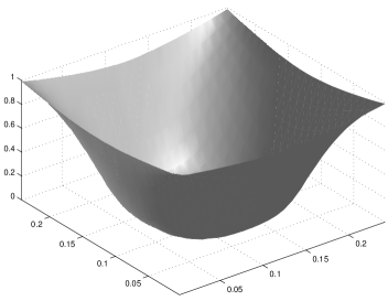
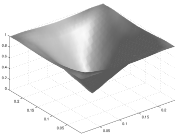
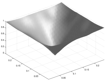
FIG. 1.: Evolution of a monopole configuration with winding number $N=1$. The vertical axis represents $|\phi|$, the horizontal plane is the x-y plane. Although the winding number is constant, the monopole core oscillates in width.

IV Results and Discussion

A Stability of an Embedded Domain Wall

Five years ago, Barriola, Vachaspati and Bucher [20] showed that a new class of non-topological defects, embedded defects, can exist in many field theories, in particular in the electroweak theory. They are solutions of the field equations. In a theory with vacuum manifold ${\cal M}$, embedded defects correspond to topological defects of a theory whose vacuum manifold is a submanifold of ${\cal M}$. Typically, they correspond to configurations in which some of the fields of the full theory are set to zero by hand. As was shown analytically in [20], embedded defects are unstable to perturbations of the field configuration. Our embedded wall (6) is an example of an embedded defect. The domain wall (6) is an embedded defect and is unstable precisely because the $Z_{2}$ which is broken is a subgroup of O(3).

Our embedded domain wall (6) is a two dimensional membrane that interpolates between two disjoint vacua $\phi_{\pm}$ which are out of phase by $180^{o}$. Figure 2 shows the time evolution of the energy density of the field configuration. By tracking the energy density we found that, independent of the spatial and temporal resolution and of the thickness of the wall core, the embedded wall (6) splits up into two walls which attain equal and opposite velocities. This splitting can be understood as follows. Initially, at the center of the wall the field is at a local maximum of the potential energy density. The forces which render the embedded wall unstable want to bring the field into a vacuum state. The forces are strongest in the core of the wall, and hence it is along the core that the fields will move away from their original values fastest. As this happens, the potential energy is transformed into kinetic and gradient energy. The induced field gradients will then act on the points to the right and to the left of the core and will start to pull them into the potential valley with them. Thus, gradient/kinetic energy waves are generated which propagate away from the original embedded wall position with the speed of light. Note that in the case of planar symmetry these new “walls” carry zero monopole winding number (because the field configuration will lie on a one-dimensional subset of the vacuum manifold). Note that this behavior of the unstable embedded wall occurs also for periodic boundary conditions.

The splitting of the embedded wall configuration will make the description of monopole-wall interaction more complicated. In the presence of a monopole, the planar symmetry of the wall gets destroyed, and then the two gradient/kinetic energy walls may well acquire a fractional winding number, as will be illustrated below. The tracking of the winding number density of the monopole-wall configuration becomes more difficult. Note that the splitting of the embedded wall occurs before the fields feel the reflective boundary conditions. Note also that the coherence of the domain walls survives long enough to be able to study the monopole-wall interaction.

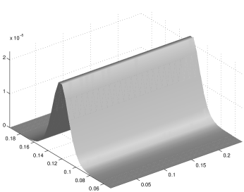
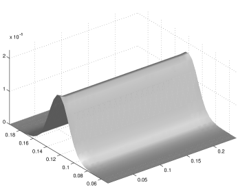
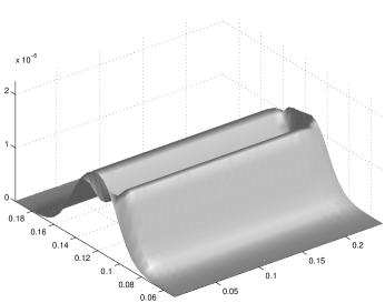
FIG. 2.: The evolution of a free domain wall. Eventually the initial wall splits into two energy walls with equal magnitude but oppositely oriented velocities.

B Attractive Force between the Monopole and Domain Wall

We studied the monopole-wall interaction by starting with the static configuration of (7) corresponding to the product ansatz of a monopole at rest and an embedded wall at rest (with $A=-1$). By observing the evolution of the energy density as a function of time in the x-y plane (Figure 3) it is possible to partially address the nature of the domain wall- monopole interaction.

From the numerical results shown in Figure 3 it follows that there is an attractive force between the monopole and the wall. If the distance between the monopole and the wall is large, then the core of the monopole evolved in an identical way to the free monopole evolution which was previously discussed in the previous section. However, if the distance is small, then this is not the case. Beginning in the second time step shown in Figure 3, it becomes clear that the presence of the wall will distort the monopole configuration (which, in the absence of the wall, was stable). The energy density peak of the monopole splits, with one peak being pulled towards the domain wall. This peak which at later times carries most of the monopole energy merges with the wall. As can be seen in the last graph, the energy is absorbed by the wall. There is no reflection. The wall persists and continues to sweep across the grid until it reflects off the edge of the target space. We have verified that the attractive force exists for both signs of $A$ in (7). Furthermore, there is an identical attractive force between the embedded wall and the antimonopole.

One way to understand the origin of the attractive force, is to perform an adiabatic analysis and consider the total gradient energy as a function of the separation $s$ between the wall and the monopole. The total gradient energy decreases as $s$ decreases. Therefore, since the field configuration tends to minimize its gradient energy, there will be an attractive force. The decrease in the total gradient energy can be seen as follows. Consider the configuration (7) with $A=-1$. By sketching the field configuration (see Figure 4) it is easy to convince oneself that as long as $s>r_{c}$, it is mostly the gradient energy of the wall which is effected by the separation $s$. Note that while $|\phi|$ is fixed, only the sign of the field component $\phi_{2}$ changes as we cross the embedded wall, and it is only this change which contributes to the gradient energy. As $s$ decreases, the area of the wall where $\phi_{2}$ is large also decreases, and hence the total gradient energy decreases. The decrease in gradient energy density is not uniform in $\rho={\sqrt{(x^{2}+z^{2})}}$, but it is sharpest near the edges of the box, as is evident from Figure 3, where it can be seen that the wall energy rapidly falls off as $x$ approaches the edges of the box.

Although this examination of the energy density of the field configurations is important in establishing the attractive force between wall and monopole, it is not enough to verify more subtle effects, like the possible unwinding of the monopole charge or monopole creation and annihilation. In particular, it is not possible to decide if the second peak in the monopole density (the one further away from the wall) is radiation or if it still carries some winding number. Topological analyses are neccessary to probe these issues.

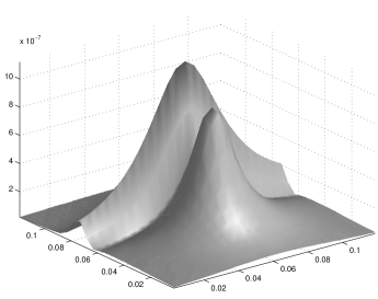
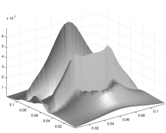
FIG. 3.: Time evolution of the energy density for the initial configuration (7) with $A=-1$. This shows the dynamics of the domain wall - monopole interaction.The monopole experiences an attractive force towards the domain wall and is stuck to it, and most of the energy density of the monopole is dispersed onto the wall.

C Unwinding of the Monopole on the Wall

The question of whether or not the monopole unwinds on the doman wall surface requires a careful investigation of the winding number evolution over the entire space. The protocol for investigating the winding evolution is as follows:

1. The winding density over the entire coordinate space is evaluated in order to determine where the winding number is localized.

2. The integrated surface winding is evaluated for a surface surrounding the monopole and one surrounding the central section of the wall, separately. At the same time, as a test of total winding number conservation, the winding over the surface of the box is computed.

3. The winding is tracked on the entire surface of the wall as well as around a gaussian surface of the monopole to check for unwinding events.

FIG. 4.: A plot of the phase of $\phi$ in the x-y plane for the configuration (7). The domain wall runs horizontally across the plot, and the monopole is situated beneath it.

By tracking the surface winding we confirm that the total winding over the entire space for the monopole and wall configuration (7) is conserved. Its value is 0.9. The difference from the naively expected value of 1 is due to edge effects - where the wall hits the surface of the box the field is not in the vacuum manifold, and hence the usual argument for the quantization of the winding number breaks down. That the total winding is (almost) 1 is to be expected since the domain wall has zero winding and the monopole has a winding of one.

The evolution of the winding number density over time is shown in Figure 5. We see that as the monopole approaches the wall, a negative image winding builds up in the center of the wall. This can be understood from the sketch of Figure 4. If we track the phase of $\phi$ ( as a phase in the $\phi_{1}-\phi_{2}$ plane intersecting the vacuum manifold ${\cal M}$) along a circle in the x-y plane about the center of the monopole, going in counter-clockwise direction, then the phase increases monotonically from $0$ to $2\pi$. This corresponds to a winding number $N=1$. However, if we consider a circle in the same plane of coordinate space surrounding the center of the wall, the phase decreases monotonically from $\pi$ to $-\pi$, corresponding to a winding number of $N=-1$.

The emergence of a negative image winding on the wall provides another way of explaining the attractive force between the monopole and the wall. The monopole sees a virtual anti-monopole on the surface of the wall and is attracted to it. It is also now obvious why, as is seen in the third frame of Figure 5, the monopole charge unwinds on the wall. After the $N=1$ winding of the monopole and the $N=-1$ image winding on the wall annihilate, the remnant winding which adds up to $N=1$ is left behind on the outer regions of the wall.

Note that an analysis of the winding density in the x-y plane (see Figure 6) shows that the second peak in the energy density of the evolved monopole (see Figure 3) carries no winding and thus corresponds to radiation.

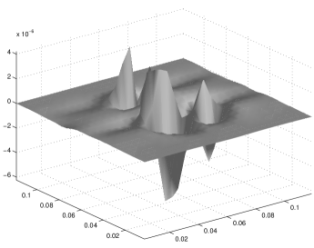
FIG. 5.: Topological charge density as a function of time for a monopole interacting with a domain wall. The monopole induces an image charge on the surface of the domain wall. Eventually, the monopole unwinds on the surface of the wall. Note that the scale of the $z$ axis differs between the subplots.

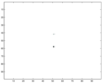
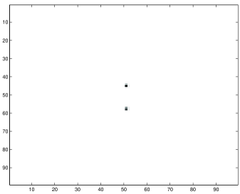
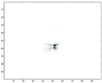
FIG. 6.: Another view of the topological charge density in the x-y plane for the initial configuration (7) and its time evolution. From this set of frames we see that the monopole winding is attracted to the wall. The magnitude of the charge density is plotted. Black represents the maximum absolute value of the winding density in each subplot.

V Conclusions

We have studied the interaction of a global monopole with an embedded wall in a $O(3)$ linear sigma model whose symmetry is spontaneously broken to $SO(2)$ by the Higgs mechanism. Our main conclusions are the following:

1. There is an attractive force between the monopole and domain wall.

2. The monopole charge unwinds on the surface of the domain wall.

We have explained the attractive force as being a result of the buildup of a negative image winding number on the wall. This image charge production also explains why the monopole charge unwinds on the wall upon contact, rather than the monopole simply scattering off the wall.

Our results should also carry over to the more complicated but physically more interesting models with local monopoles and topologically stable walls as long as monopoles and walls are (partially) made up of the same fields. Our results thus support the new solution of the monopole problem proposed by Dvali et al. [15].

REFERENCES

- [1] G. ’t Hooft, Nucl. Phys. B79, 276 (1974).
- [2] A. Belavin, A. Polyakov, A. Shvarts and Yu. Tyupkin, Phys. Lett. 59B, 85 (1975).
- [3] Ya. B. Zel’dovich and M. Yu. Khlopov, Phys. Lett. 79B, 239 (1978).
- [4] J. Preskill, Phys. Rev Lett. 43, 1365 (1979).
- [5] A. Guth, Phys. Rev. D23, 347 (1981)
- [6] J. Traschen and R. Brandenberger, Phys. Rev. D42, 2491 (1990).
- [7] L. Kofman, A. Linde and A. Starobinsky, Phys. Rev. Lett. 73, 3195 (1994).
- [8] L. Kofman, A. Linde and A. Starobinsky, Phys. Rev. Lett. 76, 1011 (1996).
- [9] I. Tkachev, Phys. Lett. B376, 35 (1996).
- [10] S. Kasuya and M. Kawasaki, Phys. Rev. D56, 7597 (1997).
- [11] M. Parry and A. Sornborger, hep-ph/9805211.
- [12] P. Langacker and S-Y. Pi, Phys. Rev. Lett. 45, 1 (1980).
- [13] J. Iliopoulos, D. Nanopoulos and T. Tomaras, Phys. Lett. 94B, 141 (1980).
- [14] G. Dvali, A. Melfo and G. Senjanovic, Phys. Rev. Lett. 75, 4559 (1995).
- [15] G. Dvali, H. Liu, and T. Vachaspati, hep-ph/9710301
- [16] M. Barriola, T. Vachaspati and M. Bucher, Phys. Rev. D50, 2819 (1994).
- [17] S. Carroll and M. Trodden, Phys. Rev. D57, 5189 (1998)
- [18] M. Maggiore, A. Riotto, hep-th/9811089.
- [19] A. Vilenkin and E.P.S Shellard, “Cosmic Strings and Other Topological Defects” (Cambridge University Press, Cambridge, 1994).
- [20] M. Barriola, T. Vachaspati and M. Bucher, Phys. Rev. D50, 2819 (1994).